

Structural and Spectroscopic Properties of Magnolol and Honokiol–Experimental and Theoretical Studies

 ,
,  ,
,  ,
,  , , , ,
  , and
, and 
Abstract
1. Introduction
2. Results and Discussion
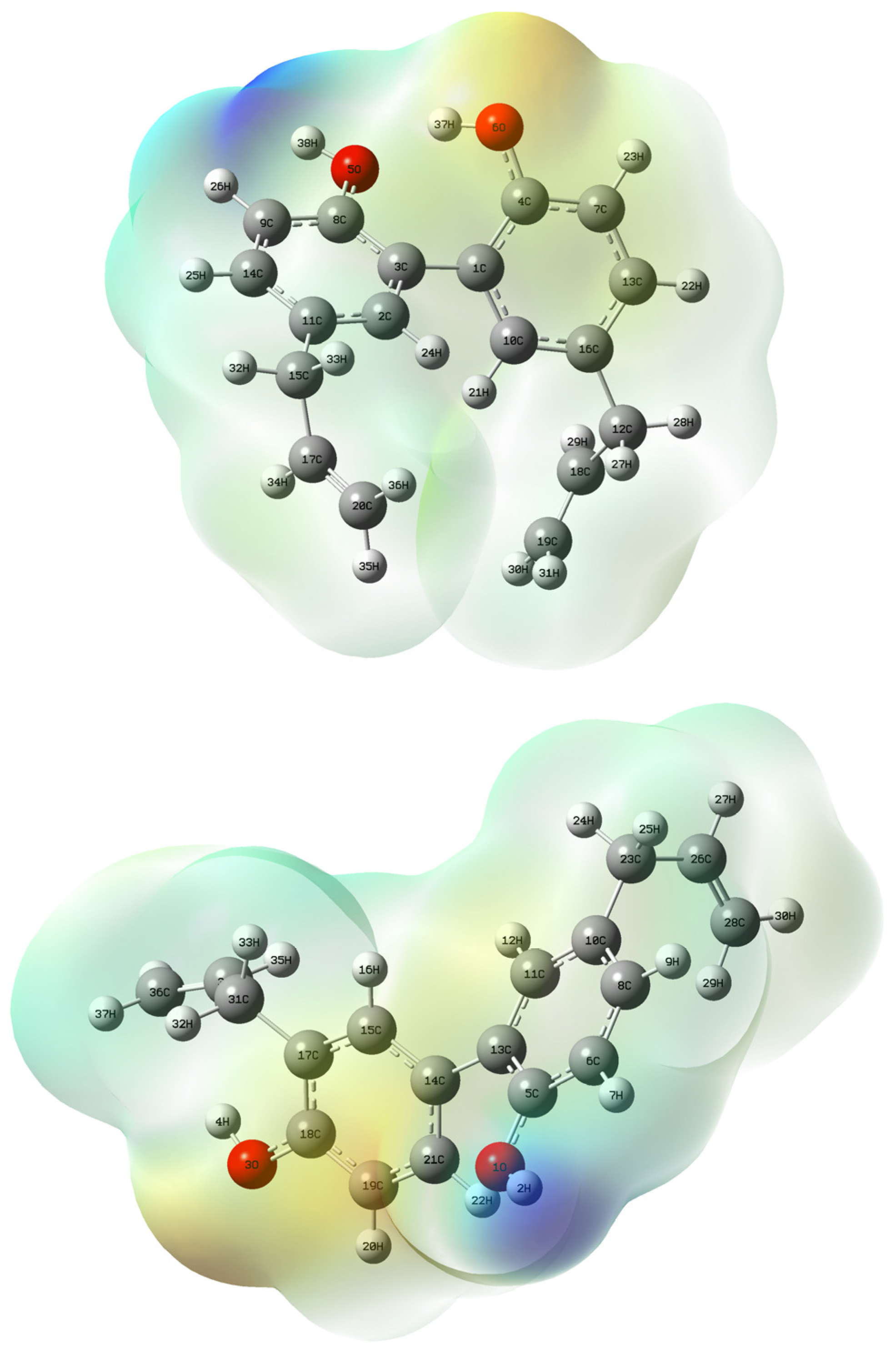
2.1. Geometry Optimization
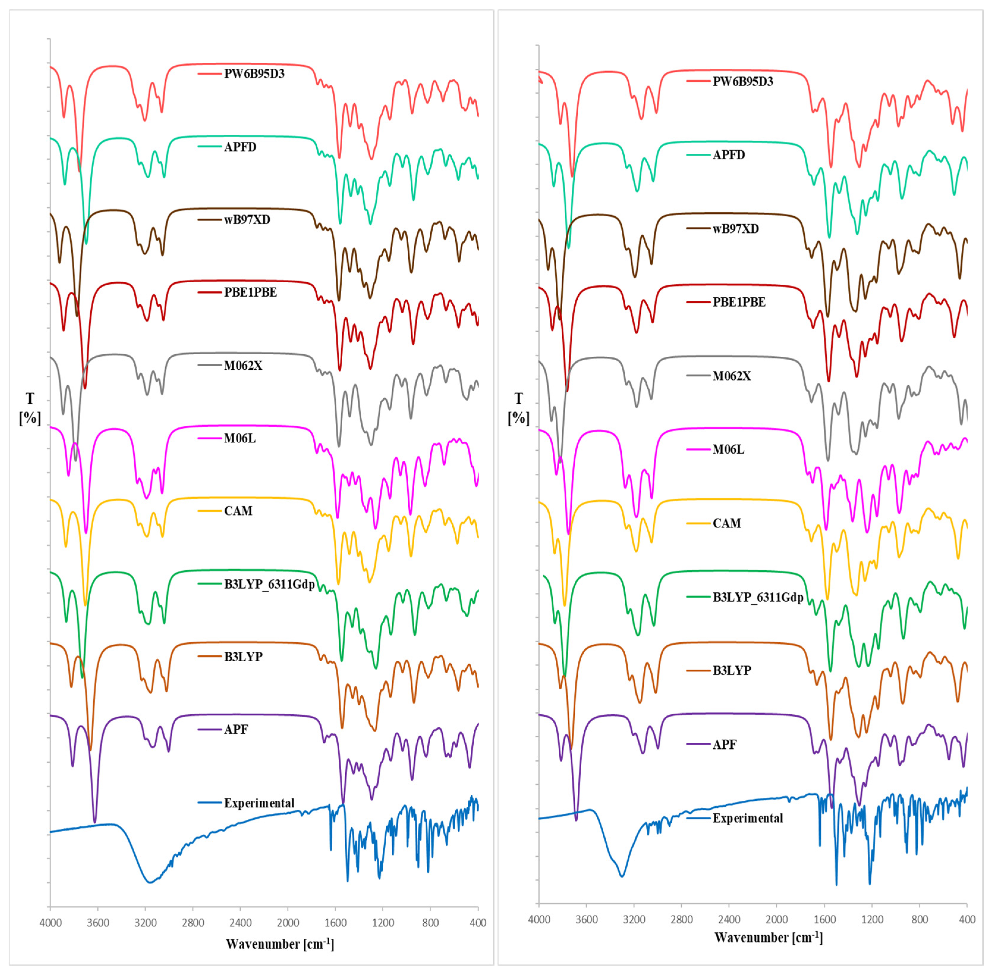
2.2. IR Analysis
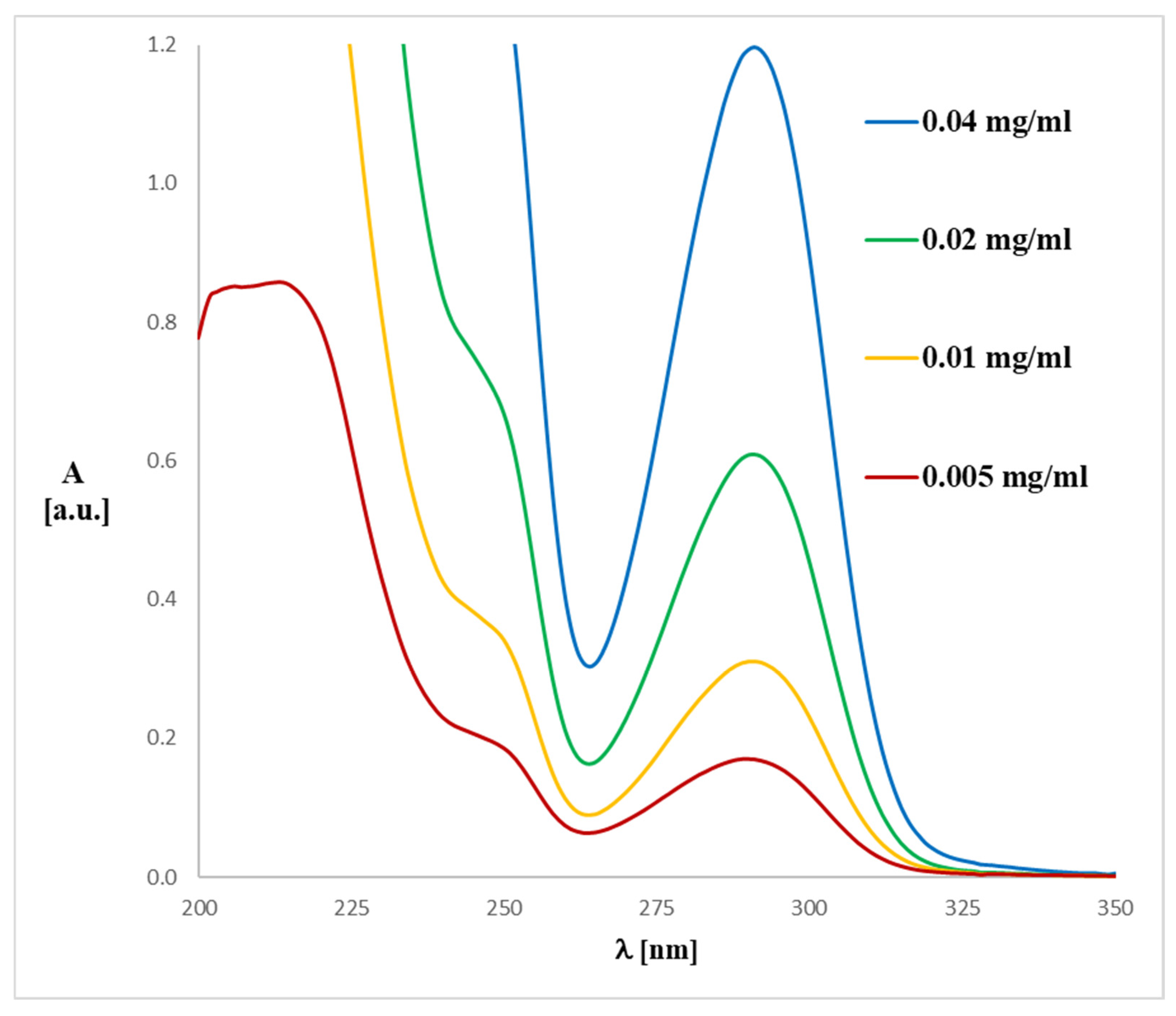
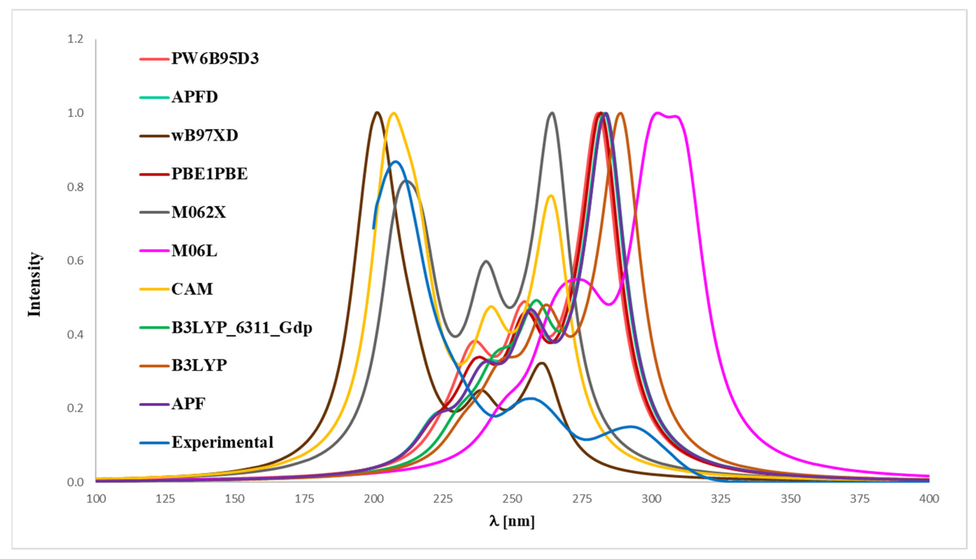
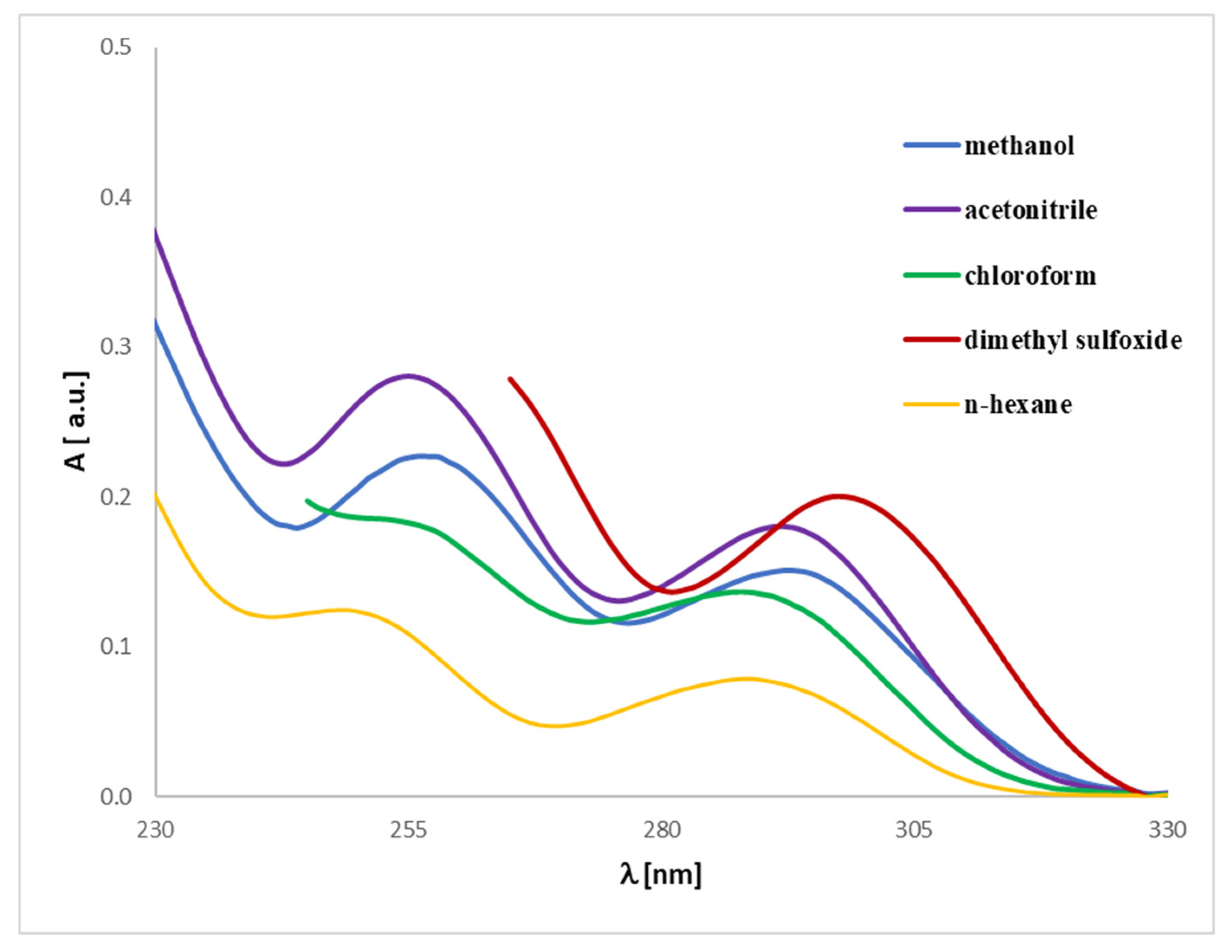
2.3. UV-Vis Analysis
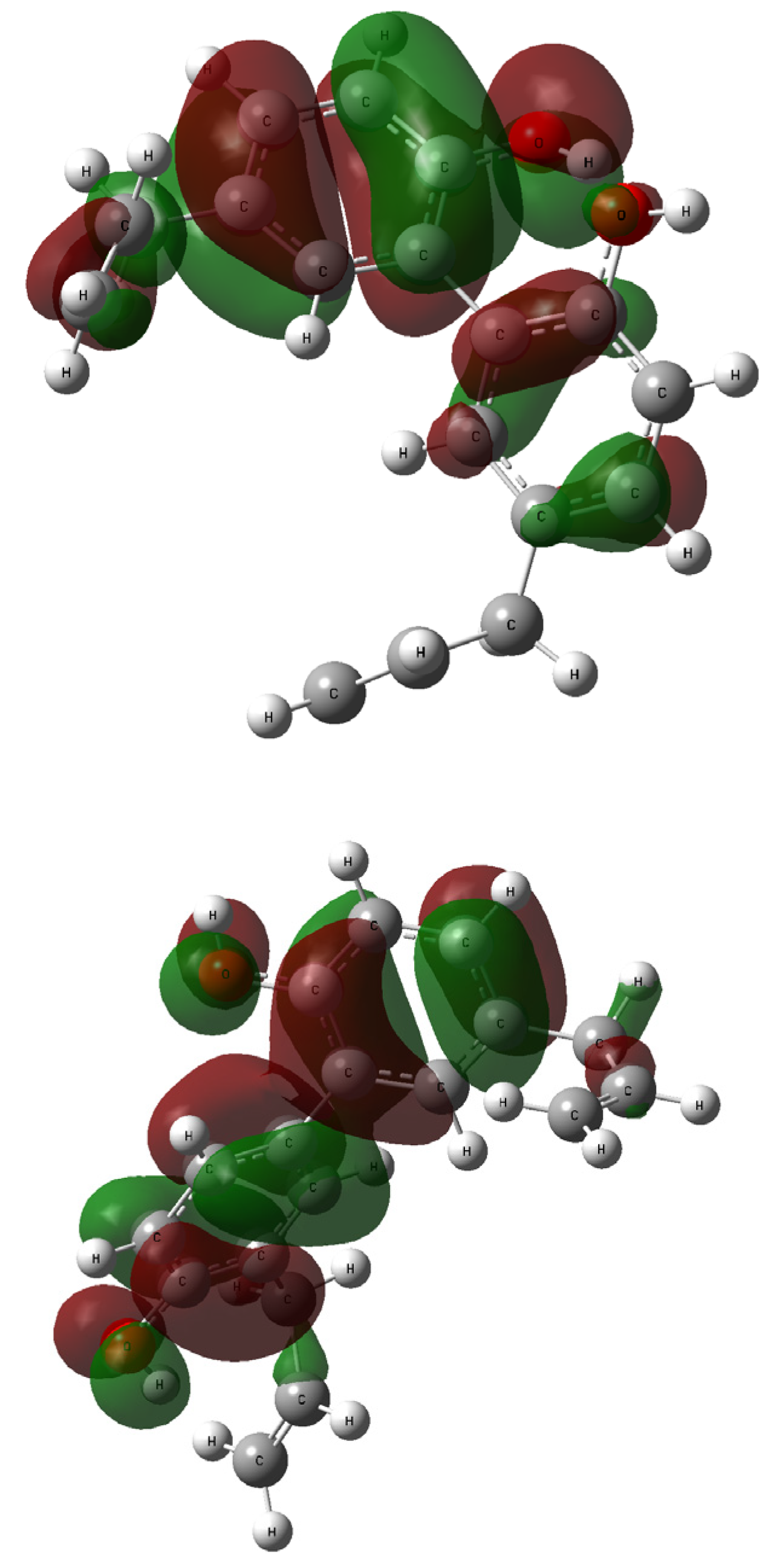
2.4. NBO Analysis
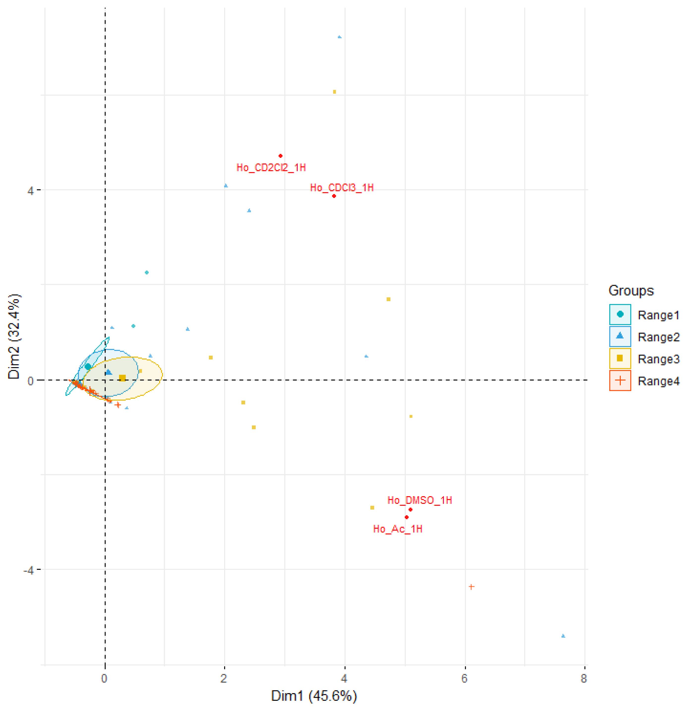
2.5. NMR Analysis
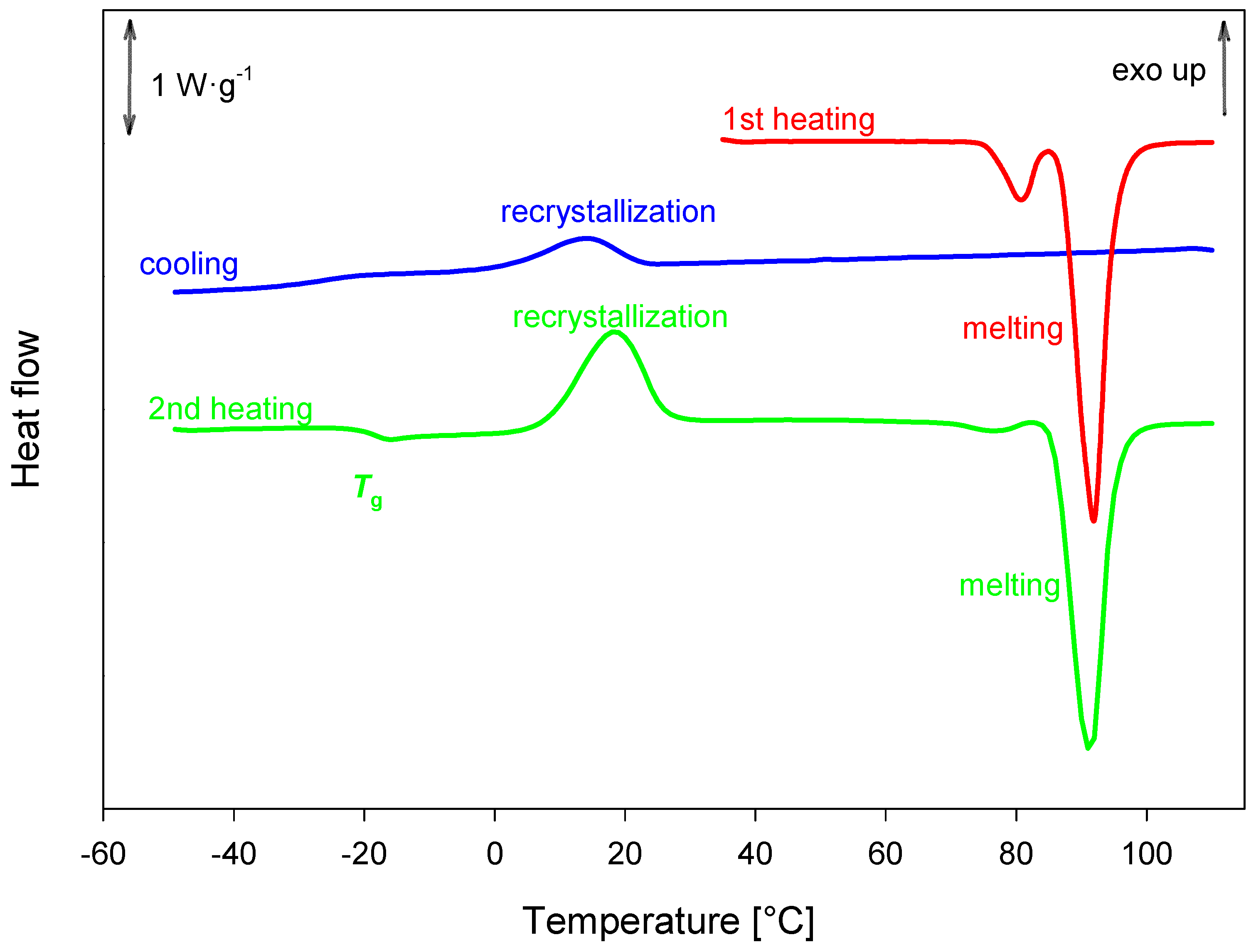
2.6. DSC Analysis
3. Materials and Methods
3.1. Chemicals
3.2. Spectroscopy
3.3. Theoretical Calculations
3.4. DSC Experiments
4. Conclusions
Supplementary Materials
Author Contributions
Funding
Institutional Review Board Statement
Informed Consent Statement
Data Availability Statement
Acknowledgments
Conflicts of Interest
Abbreviations
| FT-IR | Fourier-Transform Infrared Spectroscopy |
| UV-Vis | Ultraviolet–Visible Spectroscopy |
| NMR | Nuclear Magnetic Resonance |
| TD-DFT | Time-Dependent Density Functional Theory |
| DFT | Density Functional Theory |
| NBO | Natural Bond Orbital |
| PCA | Principal Component Analysis |
| HOMO | Highest Occupied Molecular Orbital |
| LUMO | Lowest Unoccupied Molecular Orbital |
| DSC | Differential Scanning Calorimetry |
| Tg | Glass Transition Temperature |
| ∆Cp | Change in Heat Capacity |
| ∆H | Enthalpy Change |
| BD* | Antibonding Orbital |
| RY* | Antibonding Rydberg Orbital |
| CIPXII | Crystallographic Identifier for Magnolol from CCDC |
| WIKFIF02 | Crystallographic Identifier for Honokiol from CCDC |
| CCDC | Cambridge Crystallographic Data Centre |
| MS | Mass Spectrometry |
| CDCl3 | Deuterated Chloroform (NMR solvent) |
| DMSO-d6 | Deuterated Dimethyl Sulfoxide (NMR solvent) |
| CD2Cl2 | Deuterated Dichloromethane (NMR solvent) |
| Tzero | Type of Standard Aluminum Pan (DSC equipment) |
| TMDSC | Temperature Modulated Differential Scanning Calorimetry |
References
- Harvey, A.L.; Edrada-Ebel, R.; Quinn, R.J. The re-emergence of natural products for drug discovery in the genomics era. Nat. Rev. Drug Discov. 2015, 14, 111–129. [Google Scholar] [CrossRef] [PubMed]
- Zazeri, G.; Povinelli, A.P.R.; Le Duff, C.S.; Tang, B.; Cornelio, M.L.; Jones, A.M. Synthesis and Spectroscopic Analysis of Piperine- and Piperlongumine-Inspired Natural Product Scaffolds and Their Molecular Docking with IL-1β and NF-κB Proteins. Molecules 2020, 25, 2841. [Google Scholar] [CrossRef]
- Ho, J.; Hong, C.Y. Cardiovascular protection of magnolol: Cell-type specificity and dose-related effects. J. Biomed. Sci. 2012, 19, 70. [Google Scholar] [CrossRef]
- Mottaghi, S.; Abbaszadeh, H. Natural Lignans Honokiol and Magnolol as Potential Anticarcinogenic and Anticancer Agents. A Comprehensive Mechanistic Review. Nutr. Cancer 2022, 74, 761–778. [Google Scholar] [CrossRef] [PubMed]
- Poivre, M.; Duez, P. Biological activity and toxicity of the Chinese herb Magnolia officinalis Rehder & E. Wilson (Houpo) and its constituents. J. Zhejiang Univ.-Sci. B 2017, 18, 194–214. [Google Scholar]
- Gostyńska, A.; Czerniel, J.; Kuźmińska, J.; Żółnowska, I.; Brzozowski, J.; Krajka-Kuźniak, V.; Stawny, M. The Development of Magnolol-Loaded Intravenous Emulsion with Low Hepatotoxic Potential. Pharmaceuticals 2023, 16, 1262. [Google Scholar] [CrossRef]
- Dominiak, K.; Gostyńska, A.; Szulc, M.; Stawny, M. The Anticancer Application of Delivery Systems for Honokiol and Magnolol. Cancers 2024, 16, 2257. [Google Scholar] [CrossRef] [PubMed]
- Zhang, J.; Chen, Z.; Huang, X.; Shi, W.; Zhang, R.; Chen, M.; Huang, H.; Wu, L. Insights on the Multifunctional Activities of Magnolol. BioMed Res. Int. 2019, 2019, 1847130. [Google Scholar] [CrossRef]
- Szałabska-Rąpała, K.; Borymska, W.; Kaczmarczyk-Sedlak, I. Effectiveness of Magnolol, a Lignan from Magnolia Bark, in Diabetes, Its Complications and Comorbidities—A Review. Int. J. Mol. Sci. 2021, 22, 10050. [Google Scholar] [CrossRef]
- Woodbury, A.; Yu, S.P.; Wei, L.; García, P. Neuro-Modulating Effects of Honokiol: A Review. Front. Neurol. 2013, 4, 130. [Google Scholar] [CrossRef]
- Zhao, Y.; Truhlar, D.G. Design of Density Functionals That Are Broadly Accurate for Thermochemistry, Thermochemical Kinetics, and Nonbonded Interactions. J. Phys. Chem. A 2005, 109, 5656–5667. [Google Scholar] [CrossRef] [PubMed]
- Sharanya, J.; Purushothaman, A.; Janardanan, D.; Koley, K. Theoretical exploration of the antioxidant activity of honokiol and magnolol. Comput. Theor. Chem. 2024, 1232, 114460. [Google Scholar] [CrossRef]
- Baschieri, A.; Pulvirenti, L.; Muccilli, V.; Amorati, R.; Tringali, C. Chain-breaking antioxidant activity of hydroxylated and methoxylated magnolol derivatives: The role of H-bonds. Org. Biomol. Chem. 2017, 15, 6177–6184. [Google Scholar] [CrossRef]
- Yang, Y.; Li, Z.; Zong, H.; Liu, S.; Du, Q.; Wu, H.; Li, Z.; Wang, X.; Huang, L.; Lai, C.; et al. Identification and Validation of Magnolol Biosynthesis Genes in Magnolia officinalis. Molecules 2024, 29, 587. [Google Scholar] [CrossRef]
- Murakami, Y.; Kawata, A.; Seki, Y.; Koh, T.; Yuhara, K.; Maruyama, T.; Machino, M.; Ito, S.; Kadoma, Y.; Fujisawa, S. Comparative Inhibitory Effects of Magnolol, Honokiol, Eugenol and bis-Eugenol on Cyclooxygenase-2 Expression and Nuclear Factor-Kappa B Activation in RAW264.7 Macrophage-like Cells Stimulated with Fimbriae of Porphyromonas gingivalis. In Vivo 2012, 26, 941–950. [Google Scholar]
- Wang, X.; Liu, Q.; Fu, Y.; Ding, R.-B.; Qi, X.; Zhou, X.; Sun, Z.; Bao, J. Magnolol as a Potential Anticancer Agent: A Proposed Mechanistic Insight. Molecules 2022, 27, 6441. [Google Scholar] [CrossRef]
- Kujawski, J.; Doskocz, M.; Popielarska, H.; Myka, A.; Drabińska, B.; Kruk, J.; Bernard, M.K. Interactions between indazole derivative and magnesium cations—NMR investigations and theoretical calculations. J. Mol. Struct. 2013, 1047, 292–301. [Google Scholar] [CrossRef]
- Czaja, K.; Kujawski, J.; Kujawski, R.; Bernard, M.K. DFT investigations on arylsulphonyl pyrazole derivatives as potential ligands of selected kinases. Open Chem. 2020, 18, 857–873. [Google Scholar] [CrossRef]
- Drabińska, B.; Dettlaff, K.; Ratajczak, T.; Kossakowski, K.; Chmielewski, M.K.; Cielecka-Piontek, J.; Kujawski, J. Structural and Spectroscopic Properties of Isoconazole and Bifonazole—Experimental and Theoretical Studies. Int. J. Mol. Sci. 2022, 24, 520. [Google Scholar] [CrossRef]
- Kujawski, J.; Czaja, K.; Dettlaff, K.; Żwawiak, J.; Ratajczak, T.; Bernard, M.K. Structural and spectroscopic properties of posaconazole—Experimental and theoretical studies. J. Mol. Struct. 2019, 1181, 179–189. [Google Scholar] [CrossRef]
- Najafi, M.; Najafi, M.; Najafi, H. DFT/B3LYP Study of the Substituent Effects on the Reaction Enthalpies of the Antioxidant Mechanisms of Magnolol Derivatives in the Gas-Phase and Water. Bull. Korean Chem. Soc. 2012, 33, 3607–3617. [Google Scholar] [CrossRef]
- Cossi, M.; Rega, N.; Scalmani, G.; Barone, V. Energies, structures, and electronic properties of molecules in solution with the C-PCM solvation model. J. Comput. Chem. 2003, 24, 669–681. [Google Scholar] [CrossRef]
- Deepha, V.; Praveena, R.; Sadasivam, K. DFT studies on antioxidant mechanisms, electronic properties, spectroscopic (FT-IR and UV) and NBO analysis of C-glycosyl flavone, an isoorientin. J. Mol. Struct. 2015, 1082, 131–142. [Google Scholar] [CrossRef]
- Marković, S.; Tošović, J. Application of Time-Dependent Density Functional and Natural Bond Orbital Theories to the UV–vis Absorption Spectra of Some Phenolic Compounds. J. Phys. Chem. A 2015, 119, 9352–9362. [Google Scholar] [CrossRef]
- Grimme, S.; Antony, J.; Ehrlich, S.; Krieg, H. A consistent and accurate ab initio parametrization of density functional dispersion correction (DFT-D) for the 94 elements H-Pu. J. Chem. Phys. 2010, 132, 154104. [Google Scholar] [CrossRef]
- Chandrasekaran, K.; Thilak Kumar, R. Structural, spectral, thermodynamical, NLO, HOMO, LUMO and NBO analysis of fluconazole. Spectrochim. Acta A Mol. Biomol. Spectrosc. 2015, 150, 974–991. [Google Scholar] [CrossRef]
- Austin, A.; Petersson, G.A.; Frisch, M.J.; Dobek, F.J.; Scalmani, G.; Throssell, K. A Density Functional with Spherical Atom Dispersion Terms. J. Chem. Theory Comput. 2012, 8, 4989–5007. [Google Scholar] [CrossRef] [PubMed]
- Han, J.; Li, L.; Su, M.; Heng, W.; Wei, Y.; Gao, Y.; Qian, S. Deaggregation and Crystallization Inhibition by Small Amount of Polymer Addition for a Co-Amorphous Curcumin-Magnolol System. Pharmaceutics 2021, 13, 1725. [Google Scholar] [CrossRef] [PubMed]
- He, X.; Wei, Y.; Wang, S.; Zhang, J.; Gao, Y.; Qian, S.; Pang, Z.; Heng, W. Improved Pharmaceutical Properties of Honokiol via Salification with Meglumine: An Exception to Oft-quoted ∆pKa Rule. Pharm. Res. 2022, 39, 2263–2276. [Google Scholar] [CrossRef]
- Gu, W.; She, X.; Pan, X.; Yang, T.K. Enantioselective syntheses of (S)- and (R)-8,9-dihydroxydihydromagnolol. Tetrahedron Asymmetry 1998, 9, 1377–1380. [Google Scholar] [CrossRef]
- Denton, R.M.; Scragg, J.T.; Galofré, A.M.; Gui, X.; Lewis, W. A concise synthesis of honokiol. Tetrahedron 2010, 66, 8029–8035. [Google Scholar] [CrossRef]
- Khan, P.R.; Mujawar, T.; Shekhar, P.; Shankar, G.; Subba Reddy Bv Subramanyam, R. Concise and practical approach for the synthesis of honokiol, a neurotrophic agent. Tetrahedron Lett. 2020, 61, 152229. [Google Scholar] [CrossRef]
- Li, J.; Huang, Y.; Guan, X.-L.; Li, J.; Deng, S.-P.; Wu, Q.; Zhang, Y.-J.; Su, X.-J.; Yang, R.-Y. Anti-hepatitis B virus constituents from the stem bark of Streblus asper. Phytochemistry 2012, 82, 100–109. [Google Scholar] [CrossRef]
- Bitencourt, A.S.; Oliveira, S.S.; Mendez, A.S.L.; Garcia, C.V. UV Spectrophotometric Method for Determination of Posaconazole: Comparison to HPLC. Rev. Ciênc. Farm. Básica Apl. 2015, 36. Available online: https://rcfba.fcfar.unesp.br/index.php/ojs/article/view/14 (accessed on 25 May 2025).
- Garcia, C.V. Stability-Indicating HPLC Method for Posaconazole Bulk Assay. Sci. Pharm. 2012, 80, 317–327. [Google Scholar] [CrossRef]
- Wang, Y.; Cheng, M.; Lee, J.; Chen, F. Molecular and Crystal Structure of Magnolol—C18 H18 O2. J. Chin. Chem. Soc. 1983, 30, 215–221. [Google Scholar] [CrossRef]
- Schuehly, W.; Fronczek, F.R. CCDC 986225: Experimental Crystal Structure Determination [Internet]; Cambridge Crystallographic Data Centre: Cambridge, UK, 2014; Available online: http://www.ccdc.cam.ac.uk/services/structure_request?id=doi:10.5517/cc1237q4&sid=DataCite (accessed on 25 May 2025).
- Frisch, M.J.; Trucks, G.W.; Schlegel, H.B.; Scuseria, G.E.; Robb, M.A.; Cheeseman, J.R.; Scalmani, G.; Barone, V.; Petersson, G.A.; Nakatsuji, H.; et al. Gaussian 16, Revision A.01; Gaussian, Inc.: Wallingford, CT, USA, 2009. [Google Scholar]
- Rajagopal, A.K.; Callaway, J. Inhomogeneous Electron Gas. Phys. Rev. B 1973, 7, 1912–1919. [Google Scholar] [CrossRef]
- Becke, A.D. Density-functional thermochemistry. III. The role of exact exchange. J. Chem. Phys. 1993, 98, 5648–5652. [Google Scholar] [CrossRef]
- Yanai, T.; Tew, D.P.; Handy, N.C. A new hybrid exchange–correlation functional using the Coulomb-attenuating method (CAM-B3LYP). Chem. Phys. Lett. 2004, 393, 51–57. [Google Scholar] [CrossRef]
- Lee, C.; Yang, W.; Parr, R.G. Development of the Colle-Salvetti correlation-energy formula into a functional of the electron density. Phys. Rev. B 1988, 37, 785–789. [Google Scholar] [CrossRef]
- Eckert, F.; Klamt, A. Fast solvent screening via quantum chemistry: COSMO-RS approach. AIChE J. 2002, 48, 369–385. [Google Scholar] [CrossRef]
- Perdew, J.P.; Burke, K.; Ernzerhof, M. Generalized Gradient Approximation Made Simple. Phys. Rev. Lett. 1996, 77, 3865–3868. [Google Scholar] [CrossRef] [PubMed]
- Zhao, Y.; Truhlar, D.G. A new local density functional for main-group thermochemistry, transition metal bonding, thermochemical kinetics, and noncovalent interactions. J. Chem. Phys. 2006, 125, 194101. [Google Scholar] [CrossRef]
- Zhao, Y.; Truhlar, D.G. The M06 suite of density functionals for main group thermochemistry, thermochemical kinetics, noncovalent interactions, excited states, and transition elements: Two new functionals and systematic testing of four M06-class functionals and 12 other functionals. Theor. Chem. Acc. 2008, 120, 215–241. [Google Scholar]
- Trani, F.; Scalmani, G.; Zheng, G.; Carnimeo, I.; Frisch, M.J.; Barone, V. Time-Dependent Density Functional Tight Binding: New Formulation and Benchmark of Excited States. J. Chem. Theory Comput. 2011, 7, 3304–3313. [Google Scholar] [CrossRef] [PubMed]
- Zhurko, G.A.; Zhurko, D.A. Chemcraft—Graphical Software for Visualization of Quantum Chemistry Computations [Internet]. Available online: https://www.chemcraftprog.com (accessed on 25 May 2025).
- Dennington, R.; Keith, T.; Millam, J. GaussView; Semichem Inc.: Shawnee, KS, USA, 2009. [Google Scholar]
- Siskos, M.G.; Kontogianni, V.G.; Tsiafoulis, C.G.; Tzakos, A.G.; Gerothanassis, I.P. Investigation of solute–solvent interactions in phenol compounds: Accurate ab initio calculations of solvent effects on 1H NMR chemical shifts. Org. Biomol. Chem. 2013, 11, 7400. [Google Scholar] [CrossRef]
- Abraham, R.J.; Mobli, M. An NMR, IR and theoretical investigation of1 H Chemical Shifts and hydrogen bonding in phenols. Magn. Reson. Chem. 2007, 45, 865–877. [Google Scholar] [CrossRef]


| IR Spectrum of Magnolol | ||
|---|---|---|
| Experimental Wavenumber (cm−1) | Vibrational Assignments | Calculated Wavenumber (cm−1) |
| B3LYP/6-311++G(d,p) | ||
| ca 3170 | ν OH | 3863, 3728 |
| 3123, 3073 | ν C-H arom | 3222, 3208, 3202 |
| 3053, 2930, 2835 | ν C-H alkyl | 3249, 3247, 3197, 3189, 3175, 3165, 3155, 3082, 3079, 3040, 3037 |
| 1609, 1584 | ν C-C arom | 1674, 1668, 1652, 1635, 1543 |
| 1638 | ν C=C | 1731, 1730 |
| 1282, 1155 | δ C-H arom | 1278, 1268 |
| 1243 | ν C-O asym | 1253 |
| 1047, 1020, 947 | ν C-O-C sym | 1139, 1165 |
| 849, 823, 795 | γ C-H | 1032, 975, 953, 937, 867, 752 |
| IR Spectrum of Honokiol | ||
|---|---|---|
| Experimental Wavenumber (cm−1) | Vibrational Assignments | Calculated Wavenumber (cm−1) |
| B3LYP/6-311++G(d,p) | ||
| ca 3297 | ν OH | 3902, 3822 |
| 3260 | ν C-H arom | 3261, 3243, 3226, 3212, 3207, 3202 |
| 3083, 3054, 3000, 2977 | ν C-H alkyl | 3288, 3282, 3202, 3199, 3185, 3126, 3102, 3074, 3068 |
| 1611, 1586 | ν C-C arom | 1700, 1690 |
| 1636 | ν C=C | 1754, 1743 |
| 1325, 1276 | δ C-H arom | 1309, 1304, 1245 |
| 1217 | ν C-O asym | 1226 |
| 1052 | ν C-O-C sym | 1196, 1158 |
| 918, 822, 776 | γ C-H | 954, 944, 933, 685 |
| Compound | Method | HOMO Energy | LUMO Energy | HOMO–LUMO Gap | First Ionization Potential | Electron Affinity | Chemical Potential | Chemical Hardness | Electronegativity |
|---|---|---|---|---|---|---|---|---|---|
| Magnolol | APFD | −6.0094 | −0.9197 | 5.0896 | 6.0094 | 0.9197 | −3.4646 | 2.5448 | 3.4646 |
| APF | −6.0072 | −0.9279 | 5.0793 | 6.0072 | 0.9279 | −3.4675 | 2.5396 | 3.4675 | |
| B3LYP_6311Gdp | −5.9283 | −0.9774 | 4.9508 | 5.9283 | 0.9774 | −3.4529 | 2.4754 | 3.4529 | |
| B3LYP | −5.8817 | −1.0256 | 4.8561 | 5.8817 | 1.0256 | −3.4537 | 2.4281 | 3.4537 | |
| CAM-B3LYP | −7.2252 | 0.1913 | 7.4165 | 7.2252 | −0.1913 | −3.5169 | 3.7082 | 3.5169 | |
| M062X | −7.1683 | −0.2025 | 6.9658 | 7.1683 | 0.2025 | −3.6854 | 3.4829 | 3.6854 | |
| M06L | −5.1715 | −1.4857 | 3.6858 | 5.1715 | 1.4857 | −3.3286 | 1.8429 | 3.3286 | |
| PBE1PBE | −6.0654 | −0.8558 | 5.2096 | 6.0654 | 0.8558 | −3.4606 | 2.6048 | 3.4606 | |
| PW6B95D3 | −6.1509 | −0.7788 | 5.3721 | 6.1509 | 0.7788 | −3.4648 | 2.6860 | 3.4648 | |
| wB97XD | −7.7909 | 0.8411 | 8.6320 | 7.7909 | −0.8411 | −3.4749 | 4.3160 | 3.4749 | |
| Honokiol | APFD | −6.3144 | −1.1549 | 5.1596 | 6.3144 | 1.1549 | −3.7346 | 2.5798 | 3.7346 |
| APF | −6.3204 | −1.1587 | 5.1617 | 6.3204 | 1.1587 | −3.7395 | 2.5809 | 3.7395 | |
| B3LYP_6311Gdp | −6.2216 | −1.2079 | 5.0137 | 6.2216 | 1.2079 | −3.7148 | 2.5069 | 3.7148 | |
| B3LYP | −6.1925 | −1.2446 | 4.9478 | 6.1925 | 1.2446 | −3.7186 | 2.4739 | 3.7186 | |
| CAM-B3LYP | −7.5716 | −0.0291 | 7.5425 | 7.5716 | 0.0291 | −3.8003 | 3.7712 | 3.8003 | |
| M062X | −7.5267 | −0.3899 | 7.1367 | 7.5267 | 0.3899 | −3.9583 | 3.5684 | 3.9583 | |
| M06L | −5.4540 | −1.6757 | 3.7783 | 5.4540 | 1.6757 | −3.5648 | 1.8892 | 3.5648 | |
| PBE1PBE | −6.3843 | −1.0841 | 5.3002 | 6.3843 | 1.0841 | −3.7342 | 2.6501 | 3.7342 | |
| PW6B95D3 | −6.4673 | −0.9834 | 5.4839 | 6.4673 | 0.9834 | −3.7254 | 2.7420 | 3.7254 | |
| wB97XD | −8.1169 | 0.6035 | 8.7204 | 8.1169 | −0.6035 | −3.7567 | 4.3602 | 3.7567 |
| Groups | Honokiol (Experimental Shift) | Magnolol (Experimental Shift) |
|---|---|---|
| OH | 9.33 & 9.19 ppm | 9.08 ppm, s |
| CH2–1 | (24,25-H) 3.28 ppm, d, J = 6.7 Hz, 2H | (27,28,32,33-H) 3.31 ppm, d J = 6.8 Hz, 2H |
| CH2–2 | (32,33-H) 3.37 ppm, d, J = 6.7 Hz, 2H | |
| CH–1 | (27-H) 5.98–5.91 ppm | (29,34-H) 5.93–6.01 ppm |
| CH-2 | (35-H) 5.99–6.06 ppm | |
| CH2vin–1 | (37,38-H) 5.13–5.04 ppm, tq, broad, | (30,31,35,36-H) 5.02–5.11 ppm, m |
| CH2vin–2 | (29,30-H) 5.04–4.99 ppm, m | |
| CHar | (20-H) 6.88–6.87 ppm(7-H) 6.87–6.86 ppm | (22,25-H) 6.98–7.00 ppm, (dd) J = 2.15, J = 8.20 Hz, 2H(21,24-H) 7.01–7.02 ppm, d J = 2.1 Hz, 2H |
| CHar | (9-H) 6.89–6.92 ppm, dd, J = 2.0 Hz, 8.2 Hz, 1H | - |
| CHar | (12-H) 7.02 ppm, d, J = 2.0 Hz, 1H | - |
| CHar | (22-H) 7.24–7.26 ppm, dd, J = 2.2, 8.2 Hz, 1H | (23,26-H) 6.89 ppm, d, J = 8.2 Hz, 2H |
| CHar | (16-H) 7.27–7.28 ppm, d, J = 2Hz, 1H | - |
Disclaimer/Publisher’s Note: The statements, opinions and data contained in all publications are solely those of the individual author(s) and contributor(s) and not of MDPI and/or the editor(s). MDPI and/or the editor(s) disclaim responsibility for any injury to people or property resulting from any ideas, methods, instructions or products referred to in the content. |
© 2025 by the authors. Licensee MDPI, Basel, Switzerland. This article is an open access article distributed under the terms and conditions of the Creative Commons Attribution (CC BY) license (https://creativecommons.org/licenses/by/4.0/).
Share and Cite
Kujawski, J.; Drabińska, B.; Dettlaff, K.; Skotnicki, M.; Olszewska, A.; Ratajczak, T.; Napierała, M.; Chmielewski, M.K.; Kasprzak, M.; Kujawski, R.; et al. Structural and Spectroscopic Properties of Magnolol and Honokiol–Experimental and Theoretical Studies. Int. J. Mol. Sci. 2025, 26, 6085. https://doi.org/10.3390/ijms26136085
Kujawski J, Drabińska B, Dettlaff K, Skotnicki M, Olszewska A, Ratajczak T, Napierała M, Chmielewski MK, Kasprzak M, Kujawski R, et al. Structural and Spectroscopic Properties of Magnolol and Honokiol–Experimental and Theoretical Studies. International Journal of Molecular Sciences. 2025; 26(13):6085. https://doi.org/10.3390/ijms26136085
Chicago/Turabian StyleKujawski, Jacek, Beata Drabińska, Katarzyna Dettlaff, Marcin Skotnicki, Agata Olszewska, Tomasz Ratajczak, Marianna Napierała, Marcin K. Chmielewski, Milena Kasprzak, Radosław Kujawski, and et al. 2025. "Structural and Spectroscopic Properties of Magnolol and Honokiol–Experimental and Theoretical Studies" International Journal of Molecular Sciences 26, no. 13: 6085. https://doi.org/10.3390/ijms26136085
APA StyleKujawski, J., Drabińska, B., Dettlaff, K., Skotnicki, M., Olszewska, A., Ratajczak, T., Napierała, M., Chmielewski, M. K., Kasprzak, M., Kujawski, R., Gostyńska-Stawna, A., & Stawny, M. (2025). Structural and Spectroscopic Properties of Magnolol and Honokiol–Experimental and Theoretical Studies. International Journal of Molecular Sciences, 26(13), 6085. https://doi.org/10.3390/ijms26136085