
Hierarchical Clustering and Target-Independent QSAR for Antileishmanial Oxazole and Oxadiazole Derivatives

 , ,
, ,
Abstract
:1. Introduction
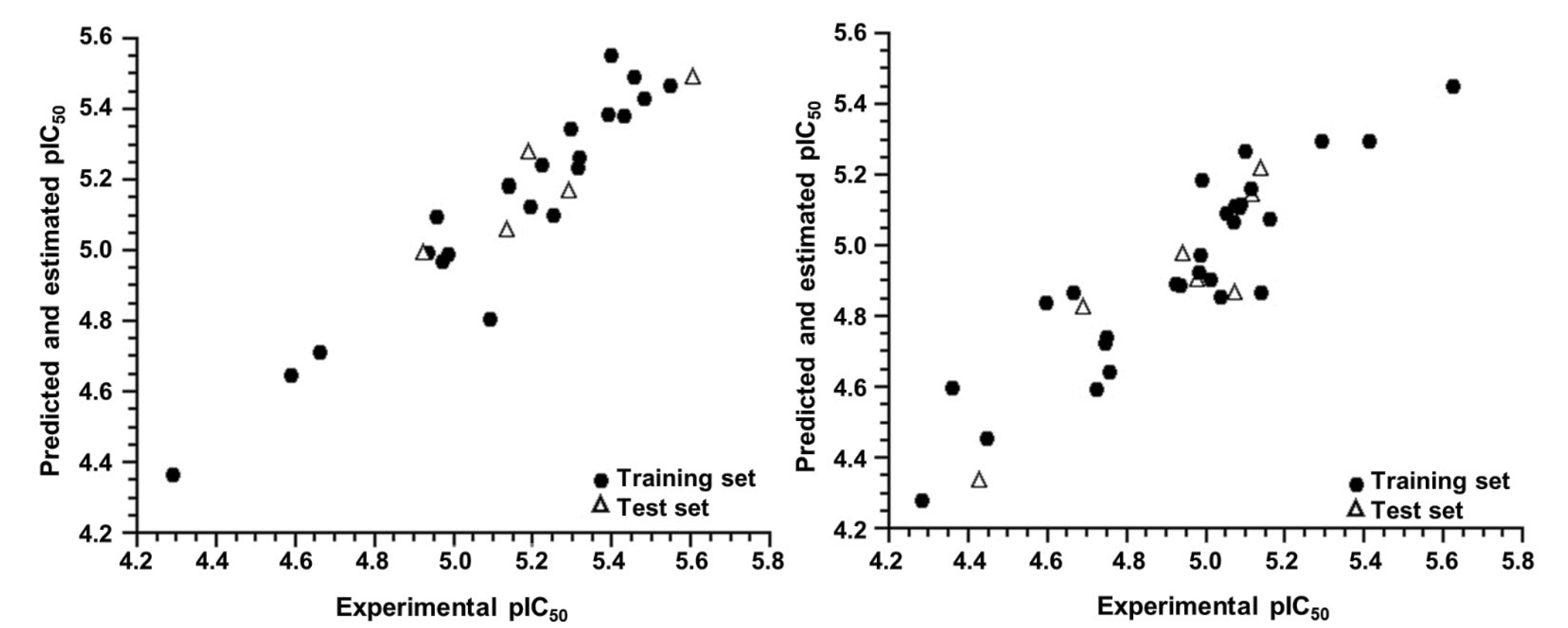
2. Results and Discussion
2.1. AutoQSAR
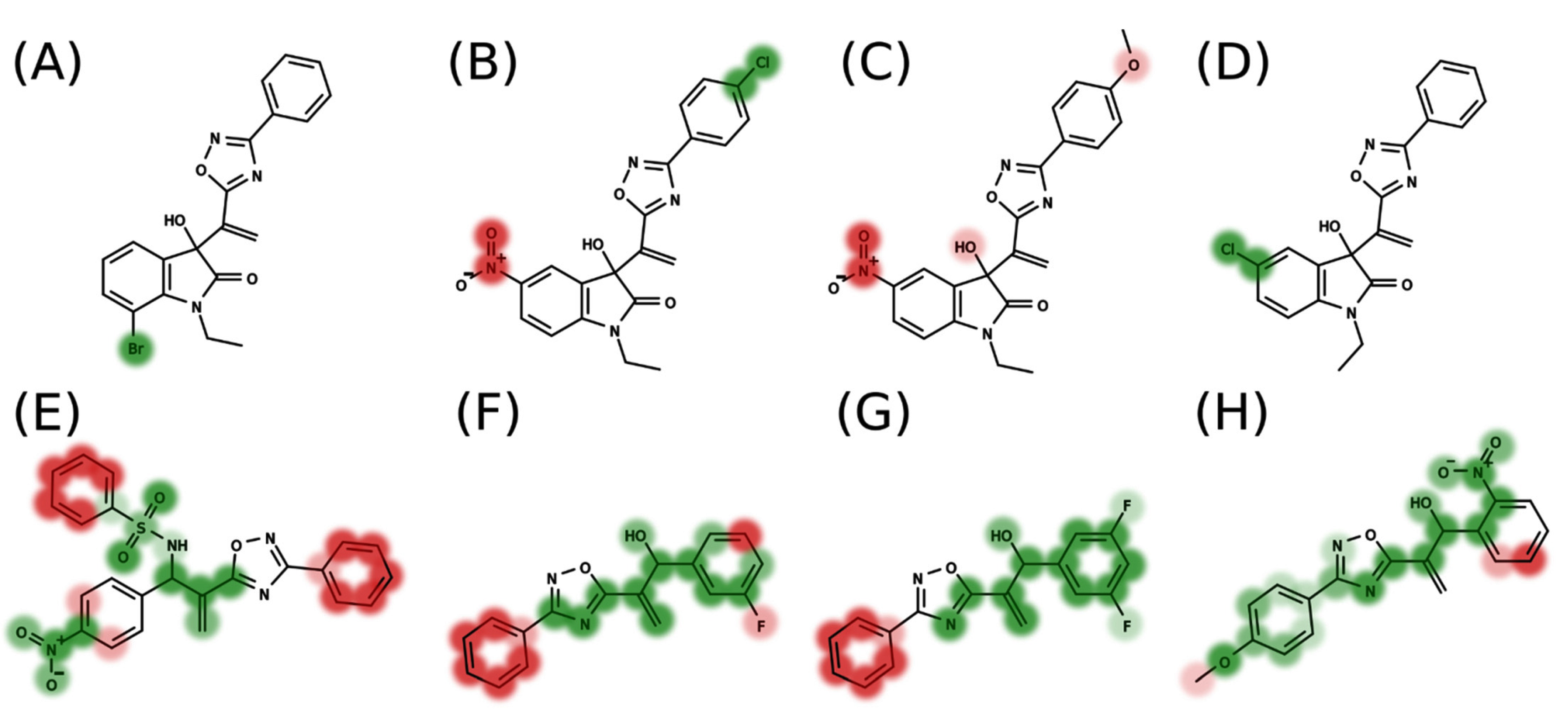
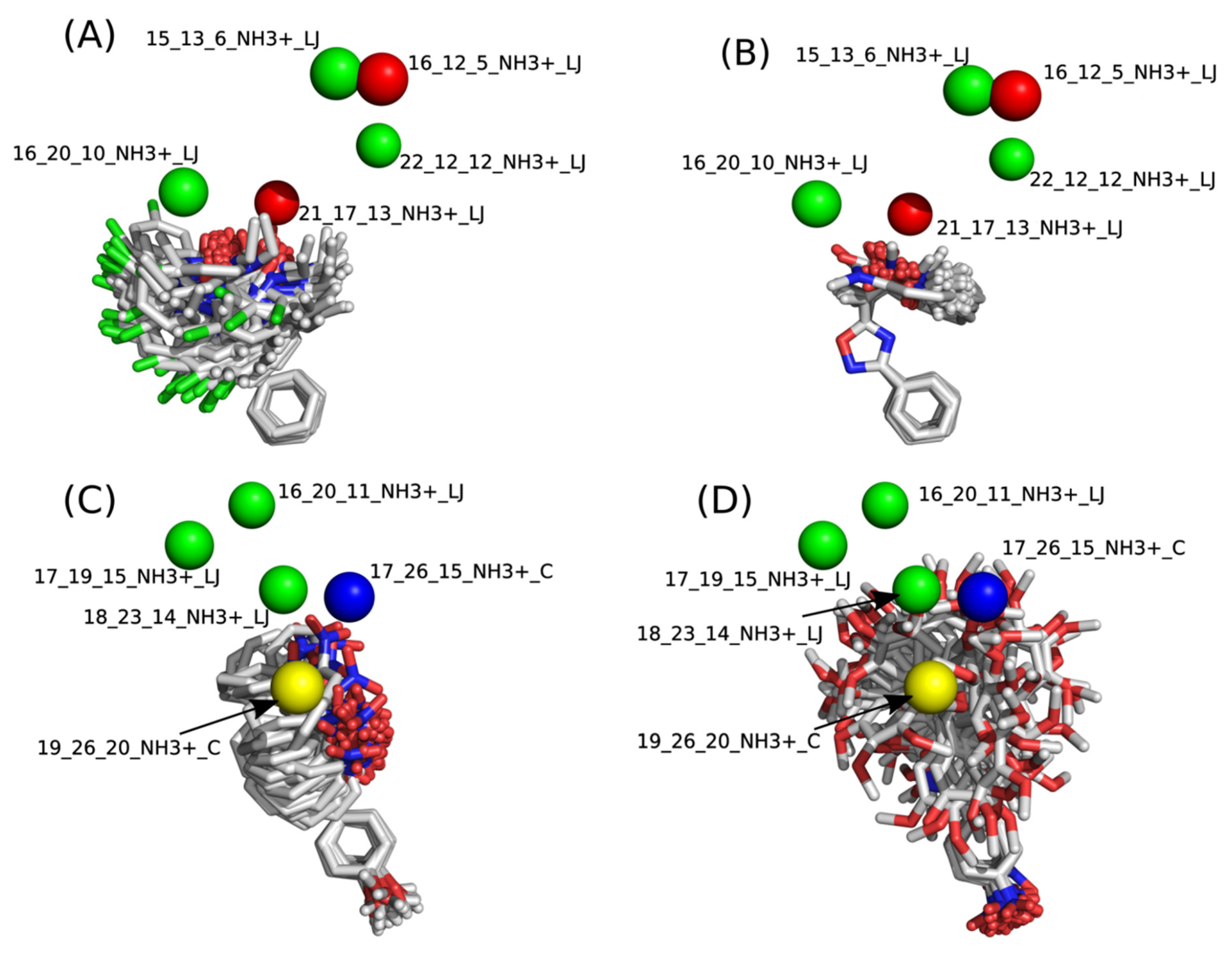
2.2. 4D-QSAR
−0.7075[16_12_5_NH3+_LJ]
+0.1484[16_20_10_NH3+_LJ]
−0.1210[21_17_13_NH3+_LJ]
+0.1913[22_12_12_NH3+_LJ]
+0.1303[17_19_15_NH3+_LJ]
−0.7328[17_26_15_NH3+_C]
+0.2770[18_23_14_NH3+_LJ]
+0.7227[19_26_20_NH3+_C]
3. Materials and Methods
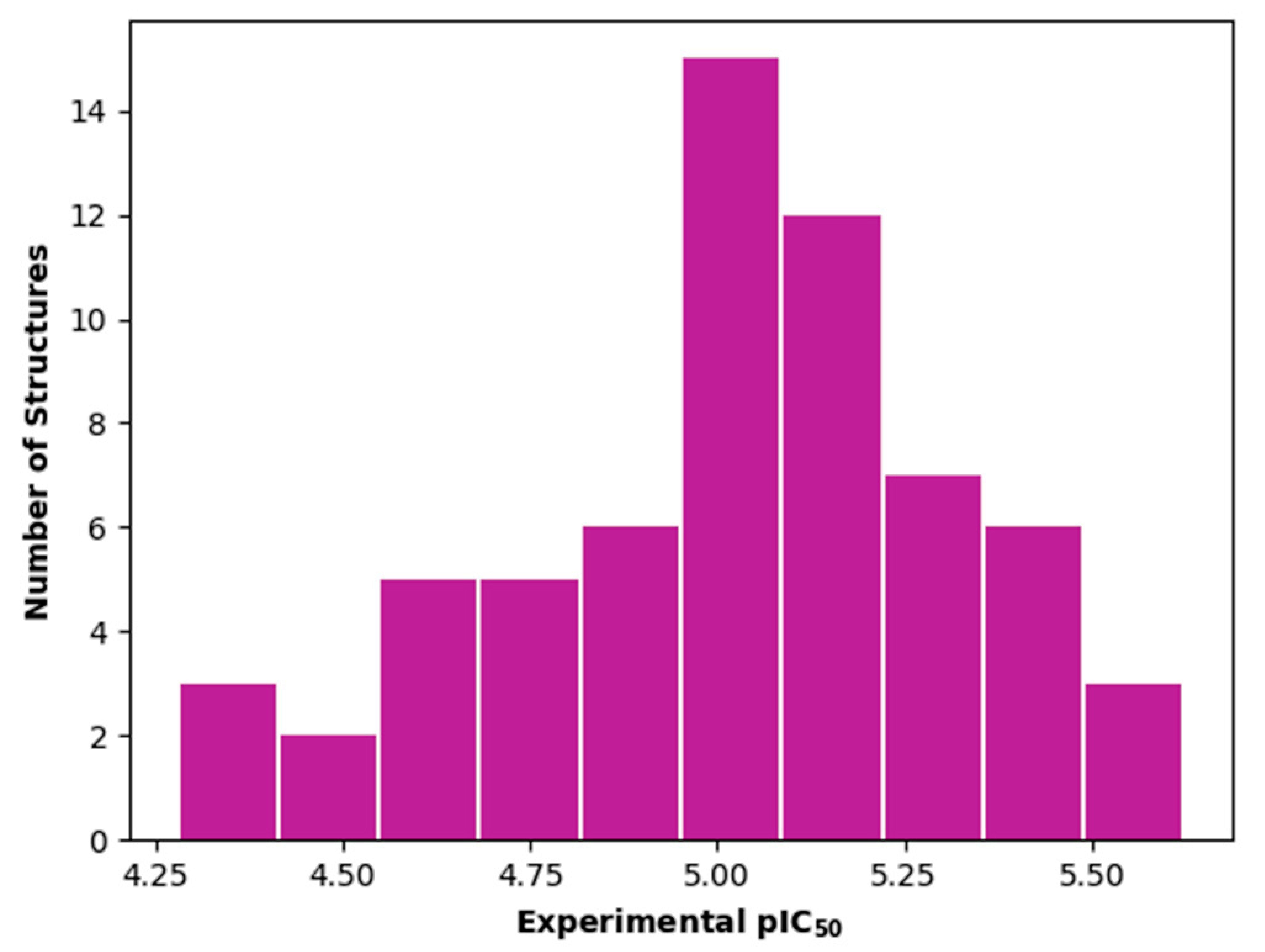
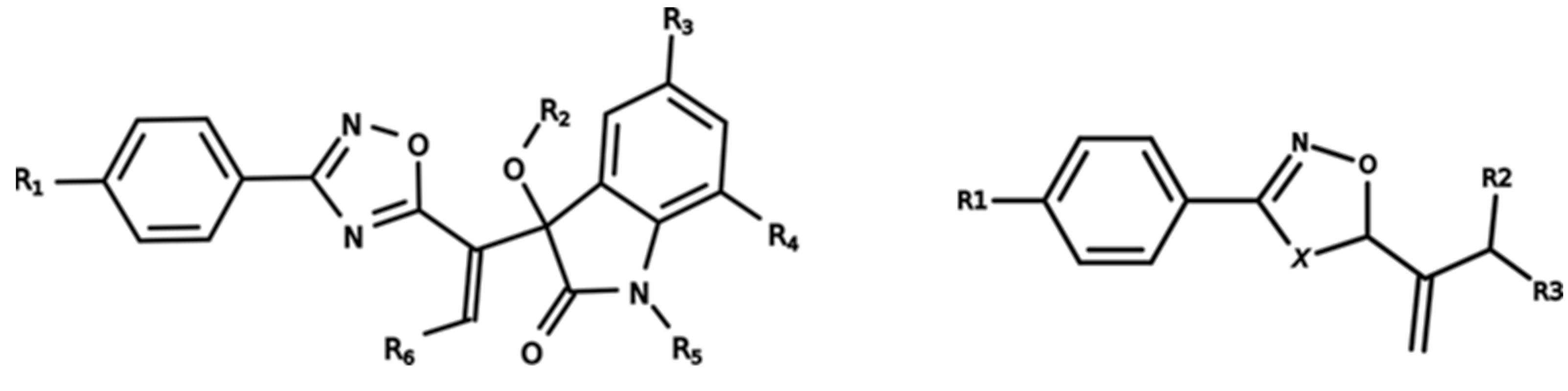
3.1. Dataset Characterization
3.2. 2D-QSAR
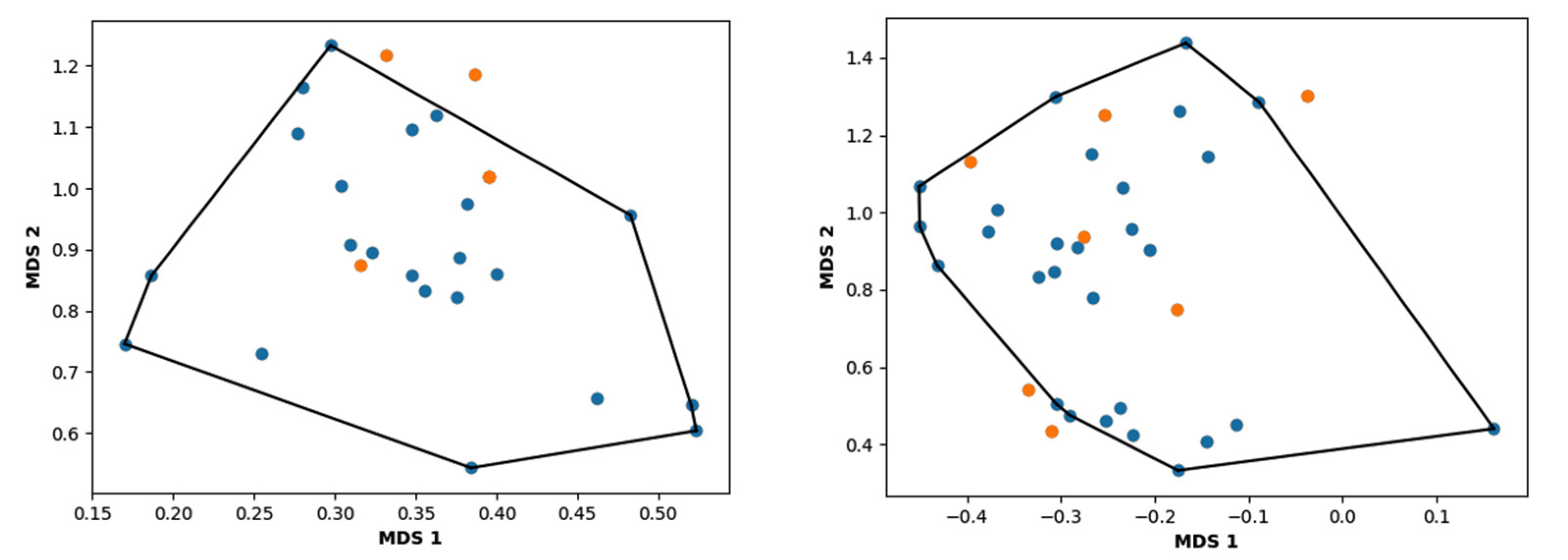
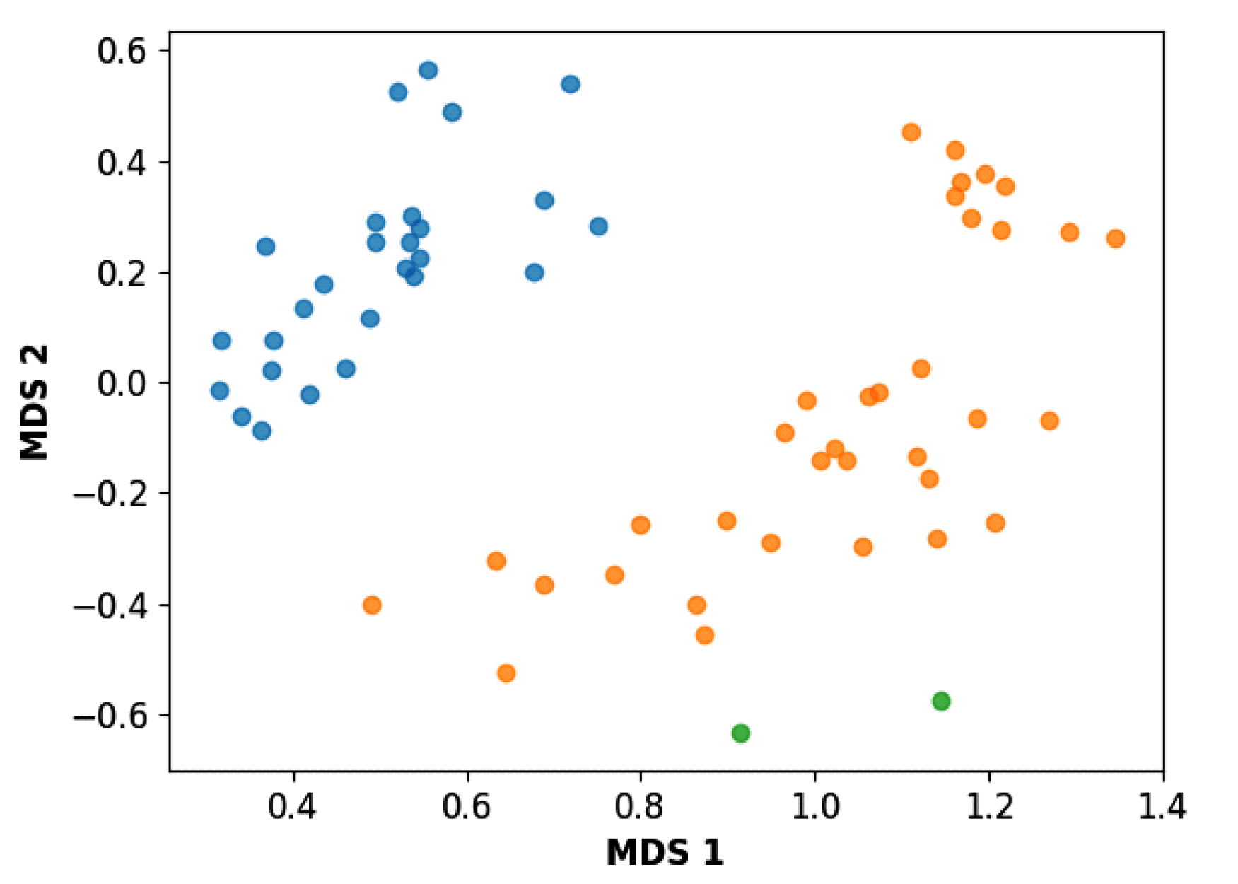
3.3. Hierarchical Clustering
3.4. 4D-QSAR
LJx,y,z ≥ 30 kcal/mol → L Jx,y,z = 30 + logLJx,y,z − 30
4. Conclusions
Supplementary Materials
Author Contributions
Funding
Institutional Review Board Statement
Informed Consent Statement
Data Availability Statement
Conflicts of Interest
References
- Ruiz-Postigo, J.A.; Grout, L.; Saurabh, J. Global leishmaniasis surveillance, 2017–2018, and first report on 5 additional indi cators/Surveillance mondiale de la leishmaniose, 2017–2018, et premier rapport sur 5 indicateurs supplementaires. Wkly. Epidemiol. Rec. 2020, 95, 265–280. [Google Scholar]
- Polonio, T.; Efferth, T. Leishmaniasis: Drug resistance and natural products. Int. J. Mol. Med. 2008, 22, 277–286. [Google Scholar] [CrossRef] [PubMed] [Green Version]
- Gourbal, B.; Sonuc, N.; Bhattacharjee, H.; Legare, D.; Sundar, S.; Ouellette, M.; Rosen, B.P.; Mukhopadhyay, R. Drug uptake and modulation of drug resistance in Leishmania by an aquaglyceroporin. J. Biol. Chem. 2004, 279, 31010–31017. [Google Scholar] [CrossRef] [Green Version]
- Fernandes, F.S.; Santos, H.; Lima, S.R.; Conti, C.; Rodrigues, M.T., Jr.; Zeoly, L.A.; Ferreira, L.L.; Krogh, R.; Andricopulo, A.D.; Coelho, F. Discovery of highly potent and selective antiparasitic new oxadiazole and hydroxy-oxindole small molecule hybrids. Eur. J. Med. Chem. 2020, 201, 112418. [Google Scholar] [CrossRef] [PubMed]
- Gilbert, I.H. Drug discovery for neglected diseases: Molecular target-based and phenotypic approaches: Miniperspectives series on phenotypic screening for antiinfective targets. J. Med. Chem. 2013, 56, 7719–7726. [Google Scholar] [CrossRef]
- Ferreira, L.L.; de Moraes, J.; Andricopulo, A.D. Approaches to advance drug discovery for neglected tropical diseases. Drug Discov. Today 2022, 27, 2278–2287. [Google Scholar] [CrossRef]
- Taha, M.; Ismail, N.H.; Ali, M.; Rashid, U.; Imran, S.; Uddin, N.; Khan, K.M. Molecular hybridization conceded exceptionally potent quinolinyl-oxadiazole hybrids through phenyl linked thiosemicarbazide antileishmanial scaffolds: In silico validation and SAR studies. Bioorganic Chem. 2017, 71, 192–200. [Google Scholar] [CrossRef]
- Taha, M.; Ismail, N.H.; Imran, S.; Selvaraj, M.; Jamil, W.; Ali, M.; Kashif, S.M.; Rahim, F.; Khan, K.M.; Adenan, M.I.; et al. Synthesis and molecular modelling studies of phenyl linked oxadiazole-phenylhydrazone hybrids as potent antileishmanial agents. Eur. J. Med. Chem. 2017, 126, 1021–1033. [Google Scholar] [CrossRef] [PubMed]
- Pitasse-Santos, P.; Sueth-Santiago, V.; Lima, M.E. 1,2,4-and 1,3,4-Oxadiazoles as Scaffolds in the Development of Antiparasitic Agents. J. Braz. Chem. Soc. 2018, 29, 435–456. [Google Scholar] [CrossRef]
- Scala, A.; Cordaro, M.; Grassi, G.; Piperno, A.; Barberi, G.; Cascio, A.; Risitano, F. Direct synthesis of C3-mono-functionalized oxindoles from N-unprotected 2-oxindole and their antileishmanial activity. Bioorganic Med. Chem. 2014, 22, 1063–1069. [Google Scholar] [CrossRef] [PubMed]
- Saha, S.; Acharya, C.; Pal, U.; Chowdhury, S.R.; Sarkar, K.; Maiti, N.C.; Jaisankar, P.; Majumder, H.K. A novel spirooxindole derivative inhibits the growth of Leishmania donovani parasites both in vitro and in vivo by targeting type IB topoisomerase. Antimicrob. Agents Chemother. 2016, 60, 6281–6293. [Google Scholar] [CrossRef] [PubMed] [Green Version]
- Kelley, L.A.; Gardner, S.P.; Sutcliffe, M.J. An automated approach for clustering an ensemble of NMR-derived protein structures into conformationally related subfamilies. Protein Eng. Des. Sel. 1996, 9, 1063–1065. [Google Scholar] [CrossRef] [PubMed] [Green Version]
- Santos-Filho, O.A.; Cherkasov, A. Using molecular docking, 3D-QSAR, and cluster analysis for screening structurally diverse data sets of pharmacological interest. J. Chem. Inf. Model. 2008, 48, 2054–2065. [Google Scholar] [CrossRef] [PubMed]
- Tropsha, A. Best Practices for QSAR Model Development, Validation, and Exploitation. Mol. Inform. 2010, 29, 476–488. [Google Scholar] [CrossRef] [PubMed]
- Hopfinger, A.; Wang, S.; Tokarski, J.S.; Jin, B.; Albuquerque, M.; Madhav, P.J.; Duraiswami, C. Construction of 3D-QSAR models using the 4D-QSAR analysis formalism. J. Am. Chem. Soc. 1997, 119, 10509–10524. [Google Scholar] [CrossRef]
- Ghasemi, J.B.; Safavi-Sohi, R.; Barbosa, E.G. 4D-LQTA-QSAR and docking study on potent gram-negative specific LpxC inhibitors: A comparison to CoMFA modeling. Mol. Divers. 2012, 16, 203–213. [Google Scholar] [CrossRef]
- Cramer, R.D.; Patterson, D.E.; Bunce, J.D. Comparative molecular field analysis (CoMFA). 1. Effect of shape on binding of steroids to carrier proteins. J. Am. Chem. Soc. 1988, 110, 5959–5967. [Google Scholar] [CrossRef] [PubMed]
- Melo, E.; Ferreira, M. A 4D structure-activity relationship model to predict HIV-1 integrase strand transfer inhibition using the LQTA-QSAR methodology. J. Chem. Inf. Model. 2012, 52, 1722–1732. [Google Scholar] [CrossRef]
- Dixon, S.L.; Duan, J.; Smith, E.; von Bargen, C.D.; Sherman, W.; Repasky, M.P. AutoQSAR: An automated machine learning tool for best-practice quantitative structure–activity relationship modeling. Future Med. Chem. 2016, 8, 1825–1839. [Google Scholar] [CrossRef]
- Release, S. Maestro; Version 3; Schrödinger LLC: New York, NY, USA, 2017. [Google Scholar]
- Medeiros, A.R.; Ferreira, L.L.; de Souza, M.L.; de Oliveira Rezende, C., Jr.; Espinoza-Chávez, R.M.; Dias, L.C.; Andricopulo, A.D. Chemoinformatics Studies on a Series of Imidazoles as Cruzain Inhibitors. Biomolecules 2021, 11, 579. [Google Scholar] [CrossRef]
- De Souza, A.S.; Ferreira, L.L.; de Oliveira, A.S.; Andricopulo, A.D. Quantitative Structure-Activity Relationships for Structurally Diverse Chemotypes Having Anti-Trypanosoma cruzi Activity. Int. J. Mol. Sci. 2019, 20, 2801. [Google Scholar] [CrossRef] [PubMed] [Green Version]
- Maggiora, G.; Vogt, M.; Stumpfe, D.; Bajorath, J. Molecular similarity in medicinal chemistry: Miniperspective. J. Med. Chem. 2014, 57, 3186–3204. [Google Scholar] [CrossRef] [PubMed]
- Berthold, M.R.; Cebron, N.; Dill, F.; Gabriel, T.R.; Kötter, T.; Meinl, T.; Ohl, P.; Thiel, K.; Wiswedel, B. KNIME—The Konstanz Information Miner: Version 2.0 and Beyond. SIGKDD Explor. Newsl. 2009, 11, 26–31. [Google Scholar] [CrossRef] [Green Version]
- Weaver, S.; Gleeson, M.P. The importance of the domain of applicability in QSAR modeling. J. Mol. Graph. Model. 2008, 26, 1315–1326. [Google Scholar] [CrossRef] [PubMed]
- Sahigara, F.; Mansouri, K.; Ballabio, D.; Mauri, A.; Consonni, V.; Todeschini, R. Comparison of different approaches to define the applicability domain of QSAR models. Molecules 2012, 17, 4791–4810. [Google Scholar] [CrossRef] [Green Version]
- Martins, J.P.A.; Barbosa, E.G.; Pasqualoto, K.F.; Ferreira, M.M. LQTA-QSAR: A new 4D-QSAR methodology. J. Chem. Inf. Modeling 2009, 49, 1428–1436. [Google Scholar] [CrossRef]
- Bekker, H.; Berendsen, H.; Dijkstra, E.; Achterop, S.; Vondrumen, R.; Vanderspoel, D.; Sijbers, A.; Keegstra, H.; Renardus, M. Gromacs-a parallel computer for molecular-dynamics simulations. In Physics Computing ’92; World Scientific Publishing: Singapore, 1993; pp. 252–256. [Google Scholar]
- Berendsen, H.J.; van der Spoel, D.; van Drunen, R. GROMACS: A message-passing parallel molecular dynamics implementation. Comput. Phys. Commun. 1995, 91, 43–56. [Google Scholar] [CrossRef]
- Schuler, L.D.; Daura, X.; van Gunsteren, W.F. An improved GROMOS96 force field for aliphatic hydrocarbons in the condensed phase. J. Comput. Chem. 2001, 22, 1205–1218. [Google Scholar] [CrossRef]
- Chandrasekhar, I.; Kastenholz, M.; Lins, R.D.; Oostenbrink, C.; Schuler, L.D.; Tieleman, D.P.; van Gunsteren, W.F. A consistent potential energy parameter set for lipids: Dipalmitoylphosphatidylcholine as a benchmark of the GROMOS96 45A3 force field. Eur. Biophys. J. 2003, 32, 67–77. [Google Scholar] [CrossRef] [PubMed]
- Parrinello, M.; Rahman, A. Crystal Structure and Pair Potentials: A Molecular-Dynamics Study. Phys. Rev. Lett. 1980, 45, 1196–1199. [Google Scholar] [CrossRef]
- Berendsen, H.J.; Postma, J.V.; van Gunsteren, W.F.; DiNola, A.; Haak, J.R. Molecular dynamics with coupling to an external bath. J. Chem. Phys. 1984, 81, 3684–3690. [Google Scholar] [CrossRef] [Green Version]
- Kim, S.; Cho, K.H. PyQSAR: A fast QSAR modeling platform using machine learning and Jupyter notebook. Bull. Korean Chem. Soc. 2019, 40, 39–44. [Google Scholar] [CrossRef] [Green Version]
- Schrödinger, LLC. The PyMOL Molecular Graphics System; Version 1.8; Schrödinger Inc.: New York, NY, USA, 2016. [Google Scholar]


| Training Set (%) | R2 | SD | Q2 (R2pred) | RMSE | N | Fingerprint |
|---|---|---|---|---|---|---|
| 70 | 0.5378 | 0.2180 | 0.4937 | 0.2123 | 1 | Radial |
| 75 | 0.5997 | 0.2065 | 0.5284 | 0.1994 | 2 | Dendritic |
| 80 | 0.6304 | 0.2022 | 0.6107 | 0.1817 | 5 | MOLPRINT 2D |
| Training Set (%) | R2 | SD | Q2 (R2pred) | RMSE | N | Fingerprint |
|---|---|---|---|---|---|---|
| 70 | 0.8982 | 0.1178 | 0.7132 | 0.1018 | 2 | Radial |
| 75 | 0.8012 | 0.1413 | 0.7022 | 0.1668 | 1 | Radial |
| 80 | 0.9069 | 0.1039 | 0.8201 | 0.0945 | 2 | Radial |
| Training Set (%) | R2 | SD | Q2 (R2pred) | RMSE | N | Fingerprint |
|---|---|---|---|---|---|---|
| 70 | 0.6109 | 0.205 | 0.4206 | 0.1829 | 2 | MOLPRINT 2D |
| 75 | 0.5693 | 0.2040 | 0.5351 | 0.1041 | 2 | MOLPRINT 2D |
| 80 | 0.8206 | 0.1377 | 0.8001 | 0.1081 | 3 | Dendritic |
| 2D-QSAR | 4D-QSAR | |||||||||
|---|---|---|---|---|---|---|---|---|---|---|
| Complete Set Model | Cluster Model | Complete Set Model | Cluster Model | |||||||
| No. | pIC50 exp | pIC50 pred | Residue | Group | pIC50 pred | Residue | pIC50 pred | Residue | pIC50 pred | Residue |
| 1 | 5.138 | 5.184 | 0.046 | G1 | 5.187 | 0.049 | 5.066 | −0.071 | 5.21 | 0.072 |
| 2 | 4.913 | 4.911 | −0.002 | - 1 | - 1 | - 1 | 4.9239 | 0.011 | - 1 | - 1 |
| 3 | 5.133 | 4.962 | −0.171 | G1 | 5.061 | −0.072 | 5.178 | 0.045 | 5.171 | 0.039 |
| 4 | 5.478 | 5.312 | −0.165 | G1 | 5.433 | −0.044 | 5.099 | −0.379 | 5.229 | −0.249 |
| 5 | 4.922 | 4.955 | 0.033 | G1 | 4.995 | 0.073 | 4.848 | −0.073 | 4.893 | −0.028 |
| 6 | 5.29 | 5.017 | −0.273 | G1 | 5.173 | −0.116 | 5.257 | −0.033 | 5.155 | −0.135 |
| 7 | 5.428 | 5.231 | −0.197 | G1 | 5.385 | −0.043 | 5.118 | −0.309 | 5.462 | 0.035 |
| 8 | 4.984 | 5.103 | 0.119 | G1 | 4.993 | 0.009 | 5.194 | 0.211 | 5.064 | 0.081 |
| 9 | 5.387 | 5.47 | 0.082 | G1 | 5.388 | −0.001 | 5.111 | −0.276 | 5.293 | −0.094 |
| 10 | 4.955 | 4.904 | −0.051 | G1 | 5.098 | 0.143 | 4.990 | 0.035 | 4.882 | −0.073 |
| 11 | 5.397 | 5.467 | 0.07 | G1 | 5.554 | 0.157 | 5.214 | −0.183 | 5.349 | −0.047 |
| 12 | 5.188 | 5.232 | 0.043 | G1 | 5.282 | 0.093 | 5.056 | −0.132 | 5.084 | −0.104 |
| 13 | 4.289 | 4.848 | 0.559 | G1 | 4.369 | 0.080 | 4.747 | 0.459 | 4.359 | 0.071 |
| 14 | 5.293 | 5.158 | −0.135 | G1 | 5.345 | 0.052 | 4.959 | −0.334 | 5.205 | −0.088 |
| 15 | 5.088 | 4.848 | −0.24 | G1 | 4.807 | −0.281 | 5.271 | 0.184 | 5.013 | −0.075 |
| 16 | 5.248 | 4.848 | −0.4 | G1 | 5.104 | 0.144 | 5.081 | −0.167 | 5.442 | 0.195 |
| 17 | 4.97 | 5.007 | 0.037 | G1 | 4.97 | 0.000 | 5.095 | 0.125 | 4.919 | −0.051 |
| 18 | 4.931 | 5.141 | 0.209 | G1 | 4.994 | 0.062 | 5.196 | 0.266 | 5.238 | 0.308 |
| 19 | 5.313 | 5.333 | 0.019 | G1 | 5.235 | −0.079 | 5.055 | −0.258 | 5.515 | 0.202 |
| 20 | 5.193 | 5.062 | −0.132 | G1 | 5.126 | −0.067 | 5.245 | 0.052 | 5.168 | −0.024 |
| 21 | 5.221 | 5.333 | 0.112 | G1 | 5.245 | 0.024 | 5.138 | −0.083 | 5.309 | 0.089 |
| 22 | 5.455 | 5.543 | 0.088 | G1 | 5.493 | 0.038 | 4.993 | −0.462 | 5.306 | −0.148 |
| 23 | 5.602 | 5.53 | −0.072 | G1 | 5.493 | −0.109 | 5.358 | −0.244 | 5.382 | −0.219 |
| 24 | 5.314 | 5.185 | −0.13 | G1 | 5.264 | −0.050 | 4.918 | −0.396 | 5.294 | −0.019 |
| 25 | 5.137 | 4.902 | −0.235 | G1 | 5.182 | 0.044 | 5.123 | −0.013 | 5.133 | −0.004 |
| 26 | 4.658 | 4.86 | 0.202 | G1 | 4.716 | 0.058 | 4.921 | 0.264 | 4.924 | 0.266 |
| 27 | 5.545 | 5.152 | −0.393 | G1 | 5.47 | −0.075 | 5.565 | 0.02 | 5.551 | 0.007 |
| 28 | 4.587 | 4.882 | 0.295 | G1 | 4.651 | 0.064 | 4.468 | −0.119 | 4.583 | −0.004 |
| 29 | 5.033 | 4.812 | −0.221 | G2 | 4.856 | −0.177 | 4.631 | −0.402 | 4.92 | −0.113 |
| 30 | 5.115 | 4.982 | −0.133 | G2 | 5.146 | 0.031 | 4.831 | −0.284 | 4.786 | −0.329 |
| 31 | 5.084 | 5.094 | 0.01 | G2 | 5.12 | 0.036 | 5.135 | 0.051 | 5.040 | −0.044 |
| 32 | 4.592 | 4.785 | 0.193 | G2 | 4.841 | 0.249 | 4.699 | 0.108 | 4.695 | 0.104 |
| 33 | 5.081 | 4.982 | −0.099 | G2 | 5.112 | 0.031 | 5.193 | 0.113 | 5.020 | −0.06 |
| 34 | 4.976 | 4.785 | −0.192 | G2 | 4.907 | −0.069 | 5.18 | 0.204 | 4.965 | −0.011 |
| 35 | 5.096 | 5.074 | −0.022 | G2 | 5.269 | 0.173 | 5.076 | −0.02 | 5.042 | −0.053 |
| 36 | 4.932 | 4.883 | −0.049 | G2 | 4.891 | −0.041 | 5.188 | 0.257 | 5.105 | 0.173 |
| 37 | 5.135 | 4.857 | −0.278 | G2 | 4.87 | −0.265 | 5.116 | −0.019 | 5.090 | −0.045 |
| 38 | 4.981 | 4.992 | 0.011 | G2 | 4.926 | −0.055 | 5.329 | 0.348 | 5.133 | 0.153 |
| 39 | 4.598 | 4.758 | 0.16 | - 1 | - 1 | - 1 | 4.5562 | −0.042 | - 1 | - 1 |
| 40 | 4.279 | 4.373 | 0.094 | G2 | 4.283 | 0.004 | 4.802 | 0.523 | 4.289 | 0.011 |
| 41 | 4.426 | 4.35 | −0.076 | G2 | 4.34 | −0.086 | 4.523 | 0.097 | 4.912 | 0.487 |
| 42 | 5.11 | 5.137 | 0.027 | G2 | 5.163 | 0.053 | 4.873 | −0.237 | 5.013 | −0.097 |
| 43 | 4.755 | 4.909 | 0.155 | G2 | 4.644 | −0.110 | 5.055 | 0.3 | 4.781 | 0.027 |
| 44 | 4.723 | 4.83 | 0.107 | G2 | 4.595 | −0.128 | 4.831 | 0.109 | 5.009 | 0.287 |
| 45 | 4.358 | 4.736 | 0.378 | G2 | 4.602 | 0.244 | 5.010 | 0.653 | 4.589 | 0.232 |
| 46 | 4.985 | 5.014 | 0.03 | G2 | 4.974 | −0.011 | 4.949 | −0.035 | 4.886 | −0.099 |
| 47 | 4.988 | 5.373 | 0.385 | G2 | 5.186 | 0.198 | 4.937 | −0.05 | 4.944 | −0.043 |
| 48 | 4.663 | 4.874 | 0.212 | G2 | 4.868 | 0.205 | 4.912 | 0.25 | 4.882 | 0.22 |
| 49 | 4.744 | 4.925 | 0.181 | G2 | 4.728 | −0.016 | 4.826 | 0.082 | 4.795 | 0.051 |
| 50 | 4.92 | 5.028 | 0.108 | G2 | 4.893 | −0.027 | 5.075 | 0.155 | 4.838 | −0.082 |
| 51 | 5.049 | 5.05 | 0.001 | G2 | 5.092 | 0.043 | 5.108 | 0.059 | 5.063 | 0.015 |
| 52 | 4.687 | 4.753 | 0.067 | G2 | 4.828 | 0.141 | 4.895 | 0.209 | 4.854 | 0.168 |
| 53 | 4.445 | 4.608 | 0.164 | G2 | 4.456 | 0.011 | 4.948 | 0.504 | 4.764 | 0.319 |
| 54 | 5.41 | 4.933 | −0.477 | G2 | 5.297 | −0.113 | 5.412 | 0.002 | 5.518 | 0.109 |
| 55 | 5.068 | 4.916 | −0.152 | G2 | 5.07 | 0.002 | 4.870 | −0.197 | 5.149 | 0.082 |
| 56 | 4.94 | 4.925 | −0.015 | G2 | 4.978 | 0.038 | 4.860 | −0.079 | 4.846 | −0.093 |
| 57 | 5.623 | 5.444 | −0.18 | G2 | 5.455 | −0.168 | 5.477 | −0.145 | 5.596 | −0.027 |
| 58 | 5.008 | 4.874 | −0.134 | G2 | 4.908 | −0.100 | 4.992 | −0.016 | 4.96 | −0.044 |
| 59 | 5.072 | 5.094 | 0.022 | G2 | 4.871 | −0.201 | 4.875 | −0.196 | 4.856 | −0.215 |
| 60 | 5.137 | 5.193 | 0.055 | G2 | 5.219 | 0.081 | 4.900 | −0.237 | 4.911 | −0.226 |
| 61 | 5.291 | 5.269 | −0.022 | G2 | 5.299 | 0.008 | 5.069 | −0.222 | 4.945 | −0.345 |
| 62 | 5.07 | 4.875 | −0.196 | G2 | 5.115 | 0.045 | 5.027 | −0.043 | 4.978 | −0.092 |
| 63 | 4.747 | 4.886 | 0.139 | G2 | 4.741 | −0.007 | 4.917 | 0.17 | 4.953 | 0.207 |
| 64 | 5.16 | 5.12 | −0.04 | G2 | 5.077 | −0.083 | 5.048 | −0.112 | 5.043 | −0.116 |
| Dataset | R2 | RMSE | Q25-fold | RMSEcv | R2pred |
|---|---|---|---|---|---|
| Complete dataset | 0.4599 | 0.2277 | 0.4137 | 0.2412 | 0.4353 |
| G1 | 0.8033 | 0.1313 | 0.6600 | 0.1716 | 0.6480 |
| G2 | 0.7005 | 0.1560 | 0.6095 | 0.1701 | 0.6581 |
| No. | Structure | pIC50 exp | No. | Structure | pIC50 exp | No. | Structure | pIC50 exp |
|---|---|---|---|---|---|---|---|---|
| 1 |  | 5.138 | 2 | 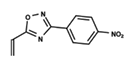 | 4.913 | 3 | 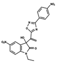 | 5.133 |
| 4 | 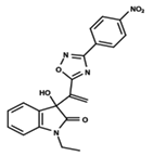 | 5.478 | 5 | 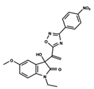 | 4.922 | 6 | 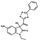 | 5.29 |
| 7 | 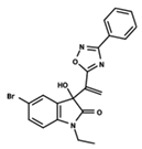 | 5.428 | 8 |  | 4.984 | 9 | 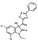 | 5.387 |
| 10 | 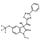 | 4.955 | 11 | 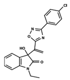 | 5.397 | 12 |  | 5.188 |
| 13 | 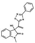 | 4.289 | 14 | 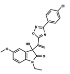 | 5.293 | 15 | 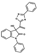 | 5.088 |
| 16 | 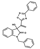 | 5.248 | 17 | 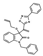 | 4.97 | 18 | 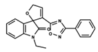 | 4.931 |
| 19 | 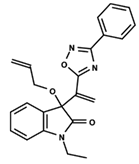 | 5.313 | 20 |  | 5.193 | 21 | 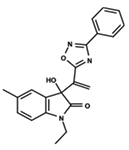 | 5.221 |
| 22 | 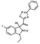 | 5.455 | 23 | 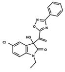 | 5.602 | 24 | 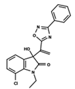 | 5.314 |
| 25 | 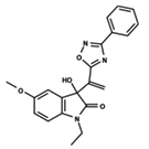 | 5.137 | 26 |  | 4.658 | 27 | 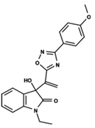 | 5.545 |
| 28 | 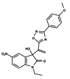 | 4.587 | 29 | 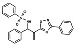 | 5.033 | 30 | 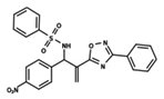 | 5.115 |
| 31 | 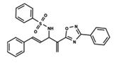 | 5.084 | 32 | 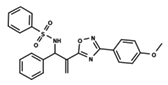 | 4.592 | 33 | 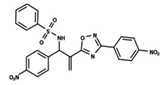 | 5.081 |
| 34 | 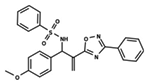 | 4.976 | 35 | 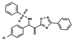 | 5.096 | 36 | 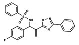 | 4.932 |
| 37 | 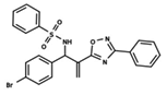 | 5.135 | 38 |  | 4.981 | 39 | 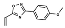 | 4.598 |
| 40 |  | 4.279 | 41 | 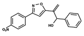 | 4.426 | 42 | 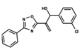 | 5.11 |
| 43 | 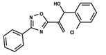 | 4.755 | 44 | 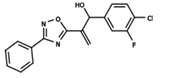 | 4.723 | 45 | 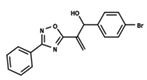 | 4.358 |
| 46 | 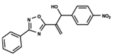 | 4.985 | 47 |  | 4.988 | 48 | 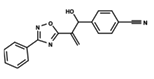 | 4.663 |
| 49 | 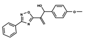 | 4.744 | 50 | 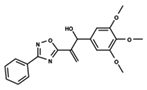 | 4.92 | 51 | 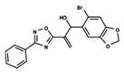 | 5.049 |
| 52 | 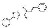 | 4.687 | 53 | 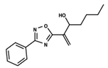 | 4.445 | 54 | 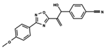 | 5.41 |
| 55 | 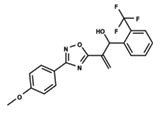 | 5.068 | 56 |  | 4.94 | 57 | 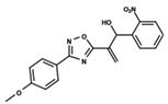 | 5.623 |
| 58 | 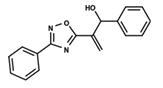 | 5.008 | 59 |  | 5.072 | 60 |  | 5.137 |
| 61 | 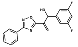 | 5.291 | 62 | 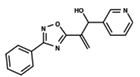 | 5.07 | 63 | 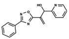 | 4.747 |
| 64 |  | 5.16 |
Publisher’s Note: MDPI stays neutral with regard to jurisdictional claims in published maps and institutional affiliations. |
© 2022 by the authors. Licensee MDPI, Basel, Switzerland. This article is an open access article distributed under the terms and conditions of the Creative Commons Attribution (CC BY) license (https://creativecommons.org/licenses/by/4.0/).
Share and Cite
Teles, H.R.; Ferreira, L.L.G.; Valli, M.; Coelho, F.; Andricopulo, A.D. Hierarchical Clustering and Target-Independent QSAR for Antileishmanial Oxazole and Oxadiazole Derivatives. Int. J. Mol. Sci. 2022, 23, 8898. https://doi.org/10.3390/ijms23168898
Teles HR, Ferreira LLG, Valli M, Coelho F, Andricopulo AD. Hierarchical Clustering and Target-Independent QSAR for Antileishmanial Oxazole and Oxadiazole Derivatives. International Journal of Molecular Sciences. 2022; 23(16):8898. https://doi.org/10.3390/ijms23168898
Chicago/Turabian StyleTeles, Henrique R., Leonardo L. G. Ferreira, Marilia Valli, Fernando Coelho, and Adriano D. Andricopulo. 2022. "Hierarchical Clustering and Target-Independent QSAR for Antileishmanial Oxazole and Oxadiazole Derivatives" International Journal of Molecular Sciences 23, no. 16: 8898. https://doi.org/10.3390/ijms23168898
APA StyleTeles, H. R., Ferreira, L. L. G., Valli, M., Coelho, F., & Andricopulo, A. D. (2022). Hierarchical Clustering and Target-Independent QSAR for Antileishmanial Oxazole and Oxadiazole Derivatives. International Journal of Molecular Sciences, 23(16), 8898. https://doi.org/10.3390/ijms23168898