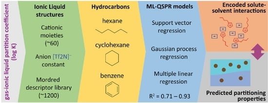
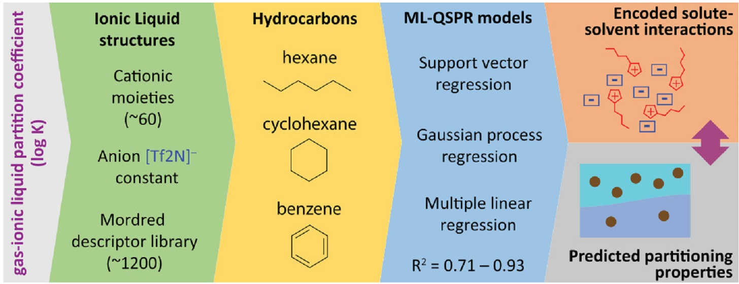
Machine Learning Quantitative Structure–Property Relationships as a Function of Ionic Liquid Cations for the Gas-Ionic Liquid Partition Coefficient of Hydrocarbons

Abstract

Ionic liquids (ILs) are known for their unique characteristics as solvents and electrolytes. Therefore, new ILs are being developed and adapted as innovative chemical environments for different applications in which their properties need to be understood on a molecular level. Computational data-driven methods provide means for understanding of properties at molecular level, and quantitative structure–property relationships (QSPRs) provide the framework for this. This framework is commonly used to study the properties of molecules in ILs as an environment. The opposite situation where the property is considered as a function of the ionic liquid does not exist. The aim of the present study was to supplement this perspective with new knowledge and to develop QSPRs that would allow the understanding of molecular interactions in ionic liquids based on the structure of the cationic moiety. A wide range of applications in electrochemistry, separation and extraction chemistry depends on the partitioning of solutes between the ionic liquid and the surrounding environment that is characterized by the gas-ionic liquid partition coefficient. To model this property as a function of the structure of a cationic counterpart, a series of ionic liquids was selected with a common bis-(trifluoromethylsulfonyl)-imide anion, [Tf2N]⁻, for benzene, hexane and cyclohexane. MLR, SVR and GPR machine learning approaches were used to derive data-driven models and their performance was compared. The cross-validation coefficients of determination in the range 0.71–0.93 along with other performance statistics indicated a strong accuracy of models for all data series and machine learning methods. The analysis and interpretation of descriptors revealed that generally higher lipophilicity and dispersion interaction capability, and lower polarity in the cations induces a higher partition coefficient for benzene, hexane, cyclohexane and hydrocarbons in general. The applicability domain analysis of models concluded that there were no highly influential outliers and the models are applicable to a wide selection of cation families with variable size, polarity and aliphatic or aromatic nature.

1. Introduction

Ionic liquids (ILs) are a special class of chemical compounds that consist of ions and commonly refer to organic salts with a low melting point [1]. The combination of exclusive properties of ionic liquids, such as extremely low vapor pressure, high polarity and thermal stability, has been a major incentive behind their study as solvents and electrolytes in synthesis [2,3,4], catalysis [2,5,6], electrochemistry [7,8,9,10,11,12,13,14], extraction and separation chemistry [4,15,16,17,18,19,20,21] and in many other applications [22,23,24,25,26]. Applications of ionic liquids often involve complex molecular systems where IL is in contact with other organic compounds. For such systems, the gas-ionic liquid partition coefficient is an important measure that characterizes the distribution of an organic compound between an ionic liquid and the surrounding environment [27]. In order to optimize partition coefficients for specific applications, new ionic liquids are continuously produced [28,29,30,31,32,33]. Thereby, characterizing the influence of the ionic counterparts of the IL and constructing gas-ionic partition coefficient models based on the molecular structure of ion counterparts is essential in order to design application-targeted ionic liquids as rapidly, cost-effectively and as precisely as possible.

The gas-ionic liquid partition coefficient, K, quantifies the distribution of a chemical compound between a gas phase and an ionic liquid [34]:

$$K=\frac{c_{IL}}{c_G},$$

(1)

where $c_G$ and $c_{IL}$ are compound concentrations in the gas phase and the ionic liquid, respectively. The partition coefficient is often provided in the logarithmic form, log K. The coefficient can be calculated from inverse gas-liquid chromatography (GLC) experiments as the ratio of the carrier gas volume used for solute elution to the stationary liquid phase volume. Experimental methods for finding K are laborious, costly, slow and require ample amounts of sufficiently pure compounds. Extensible screening efforts of compounds with application-suited log K are enabled using theoretical and computational approaches, such as quantitative structure–property relationships (QSPRs).

The literature shows that log K has been mostly modeled as a function of structure of organic compounds partitioning between gas and ionic liquid. Examples include the more commonly known Abraham solvation model [35,36,37,38,39,40,41,42,43,44,45] and a selection of linear and non-linear QSPR approaches [46,47]. Our recent research effort in this direction concentrated on modeling the gas-ionic liquid partition coefficient of a large variety of organic compounds in three ionic liquids [48]. We have previously developed a series of gas-liquid partition coefficient models for a general treatment of solubility in traditional organic solvents [49,50,51,52]. In another study, we modeled gas-liquid partition coefficients in methanol and ethanol [53]. The series of research has shown that QSPR approaches that employ theoretical molecular descriptors to study gas-liquid partition coefficients have been successful for many applications involved in physico-chemical [54,55], toxicological [56,57,58], biomedical [59,60] and material properties [61,62]. However, models for log K prediction in the scientific literature involving the ionic liquid’s molecular structure are incredibly sparse, with the only example being the ion-specific Abraham model [45]. Generally, QSPR-s concentrate on predicting the partitioning capacity of organic solvents within a specific ionic liquid [35,36,37,38,39,40,41,42,43,44,46,47]. These modeling efforts provide an understanding of partitioning interactions from the perspective of organic compounds, while the ionic liquid remains constant. On the other hand, it is equally important to understand the influence of ionic liquid structure on the partitioning properties. Thereby, characterizing the influence of the ionic counterparts of the IL and constructing gas-ionic partition coefficient models based on the molecular structure of ion counterparts are essential to design application-targeted ionic liquids as rapidly, cost-effectively and as precisely as possible. The present study tests the hypothesis that log K can also be modeled based on the partial structure of the ionic liquid. Advances in this computational modeling direction are beneficial to the ionic liquid research and development community, because such models improve the general understanding of ILs and help to design novel ILs while saving time and costs by reducing the need for experiments.

The study concentrates on modeling the gas-ionic liquid partition coefficients for three organic compounds hexane, cyclohexane and benzene in the series of ionic liquids with common bis(trifluoromethylsulfonyl)imide ([Tf2N]⁻) anion using linear and non-linear QSPR methods. [Tf2N]⁺ ILs are being extensively studied for various applications, for example as a media for supercapacitors [63], a heavy metal adsorbent [64], an anticancer agent [65] and gas solvent in sensors [66] among many other applications [67,68,69]. Variation in ionic counterpart makes it possible more specifically to understand how molecular interactions of partitioning by the ionic liquid and how to enable finding the application-appropriate ionic liquid. Hexane, cyclohexane and benzene are commonplace organic compounds, more specifically, hydrocarbons having the same number of carbon atoms but different molecular flexibility, saturation and a lack of electronegative atoms. Modeling the log K of these compounds in various ionic liquids with a constant anion allows characterizing the contributions of the structural properties of the IL cation with respect to three incrementally different solute environments. The interpretation of linear and non-linear QSPR models makes it possible to distinguish the main structural components of an ionic liquid and an organic solute that influence distribution between them.

2. Results

The optimal linear and non-linear (hyperparameters in

Table 1. Hyperparameters of the SVR and GPR final models.

	C	ε	γ
SVRh	1	0.001	auto
SVRc	5	0.001	0.1
SVRb	1	0.001	scale
	Sigma_0	Noise_Level	Length_Scale
GPRh	0.478	0.00947	3.7
GPRc	0.364	0.00888	9.52
GPRb	3.13	0.00215	2.91

) models found for hexane and cyclohexane data series showed cross-validated r² values in the range 0.89 … 0.93. The linear and non-linear models for the benzene data series resulted in cross-validated r² values in the range 0.72 … 0.85. The RMSE values for all models are within 0.05 to 0.11. All models include three to five parameters and the individual training and cross-validation statistics show high predictive capability on all validation folds (

Table 2. Statistical parameters of final linear and non-linear models on all cross-validation folds.

	R2			RMSE			CCC
	MLRh	SVRh	GPRh	MLRh	SVRh	GPRh	MLRh	SVRh	GPRh
train	0.944	0.966	0.957	0.092	0.071	0.080	0.971	0.982	0.978
test	0.919	0.926	0.924	0.101	0.098	0.097	0.960	0.957	0.957
	MLRc	SVRc	GPRc	MLRc	SVRc	GPRc	MLRc	SVRc	GPRc
train	0.915	0.946	0.940	0.102	0.081	0.085	0.955	0.972	0.969
test	0.891	0.910	0.903	0.110	0.097	0.097	0.942	0.953	0.950
	MLRb	SVRb	GPRb	MLRb	SVRb	GPRb	MLRb	SVRb	GPRb
train	0.791	0.973	0.935	0.068	0.025	0.038	0.883	0.986	0.966
test	0.717	0.869	0.788	0.072	0.051	0.057	0.813	0.928	0.869

), which can also be seen from the experimental to predicted log K plots (Figure 1, Figure 2 and Figure 3).

2.1. Models for Hexane in [Tf2N]^– Ionic Liquids

The final MLR model (Equation (2) of log K for hexane in [Tf2N]⁻ ionic liquids (MLRh) contained five molecular descriptors and had a cross-validation r²_cv10 of 0.919. The selected descriptors included the following: VE2_A (average coefficient of the last eigenvector from the distance matrix), AATS7s (averaged Moreau–Broto autocorrelation of lag 7 weighted by intrinsic state), ATSC0s (centered Moreau–Broto autocorrelation of lag 0 weighted by intrinsic state), AATSC2dv (averaged and centered Moreau–Broto autocorrelation of lag 2 weighted by valence electrons) and Xpc-4d (4-ordered Chi path-cluster weighted by sigma electrons).

$$\log K=1.417$$

$$-0.326 VE2\_A$$

$$-0.089 AATS7s$$

(2)

$$-0.126 ATSC0s$$

$$+0.06 AATSC2dv$$

$$-0.133 Xpc\text{-}4d$$

The optimal five-parameter SVR model for hexane in [Tf2N]^– ionic liquids (SVRh) showed a cross-validation r²_cv10 of 0.926, which is slightly higher than the statistics of the linear model. The selected molecular descriptors all were different in comparison with MLR model: SMR_VSA5 (sum of Crippen–Wildman molar refractivity of atoms with van der Waals surface area 2.45–2.75), AATSC0s (averaged and centered Moreau–Broto autocorrelation of lag 0 weighted by intrinsic state), SpMAD_D (spectral mean absolute deviation from distance matrix), AATS6m (averaged Moreau–Broto autocorrelation of lag 6 weighted by mass) and Xc-5d (5-ordered Chi cluster weighted by sigma electrons).

In the GPR model for hexane in [Tf2N]⁻ ionic liquids (GPRh), the optimal model was found at four parameters with a cross-validation coefficient of determination r²_cv10 of 0.924. Two of the molecular descriptors (SMR_VSA5, Xpc-4d) in the model were the same as in SVR and MLR models, respectively. The other two descriptors did not occur before: GATS1s (Geary coefficient of lag 1 weighted by intrinsic state) and ATSC1are (centered Moreau–Broto autocorrelation of lag 1 weighted by Allred–Rochow EN).

2.2. Models for Cyclohexane in [Tf2N]^– Ionic Liquids

In the optimal MLR model (Equation (3)) for cyclohexane in [Tf2N]^– ionic liquids (MLRc), cross-validation r²_cv10 was calculated to be 0.891. The model consisted of four descriptors: VE2_A, GATS7Z (Geary coefficient of lag 7 weighted by atomic number), ATSC0s and Xpc-4d.

$$\log K=1.808$$

$$-0.329 VE2\_A$$

$$-0.101GATS7Z$$

(3)

$$-0.153 ATSC0s$$

$$-0.126 Xpc\text{-}4d$$

The optimal SVR model derived for cyclohexane in [Tf2N]⁻ ionic liquids (SVRc) showed a cross-validation r²_cv10 of 0.910. The four descriptors in the model were SMR_VSA5, Xc-5d, AATSC0s and AATS7m (averaged Moreau–Broto autocorrelation of lag 7 weighted by mass).

Using five descriptors, the GPR model for cyclohexane in [Tf2N]^– ionic liquids (GPRc) achieved a cross-validation r²_cv10 of 0.903. The model consisted of molecular descriptors that were not present in previous models: SLogP (Wildman–Crippen LogP), Xpc-4dv (4-ordered Chi path-cluster weighted by valence electrons), AATS0s (averaged Moreau–Broto autocorrelation of lag 0 weighted by intrinsic state), MATS8c (Moran coefficient of lag 8 weighted by Gasteiger charge) and AATSC6se (averaged and centered Moreau–Broto autocorrelation of lag 6 weighted by Sanderson electronegativity).

2.3. Models for Benzene in [Tf2N]^– Ionic Liquids

Regarding the MLR model for benzene in [Tf2N]⁻ ionic liquids (MLRb), the optimal model (Equation (4)) is characterized by a cross-validation r²_cv10 of 0.717. Using the OMP algorithm, three descriptors were selected for the model: AATS0s (averaged Moreau–Broto autocorrelation of lag 0 weighted by intrinsic state), GATS2dv (Geary coefficient of lag 2 weighted by valence electrons) and GATS3m (Geary coefficient of lag 3 weighted by mass). None of them were present in the model for two other hydrocarbons.

$$\log K=2.791$$

$$-0.131 AATS0s$$

(4)

$$-0.055 GATS2dv$$

$$-0.042 GATS3m$$

In the case of the SVR model for benzene in [Tf2N]⁻ ionic liquids (SVRb), however, the four-parameter model showcased a cross-validation r²_cv10 of 0.851. The model included different set of the descriptors: Mi (mean of constitutional weighted by ionization potential), ATSC1s (centered Moreau–Broto autocorrelation of lag 1 weighted by intrinsic state), GATS2pe (Geary coefficient of lag 2 weighted by Pauling electronegativity) and AATSC8i (averaged and centered Moreau–Broto autocorrelation of lag 8 weighted by ionization potential).

The three-parameter GPR model for benzene in [Tf2N]^– ionic liquids (GPRb) had a cross-validation r²_cv10 of 0.788 with the descriptors AATSC0s, GATS3Z (Geary coefficient of lag 3 weighted by atomic number) and MDEC-12 (molecular distance edge between primary C and secondary C).

3. Discussion

3.1. Descriptors Interpretation

The interpretation of descriptors selected into the final models allows the analysis of the molecular structural factors that influence the gas-ionic liquid partition and interactions influenced by the cationic counterparts. The relative importance and influence of individual descriptors were analyzed using standardized regression coefficients in multiple linear regression models (Equations (2)–(4)), and the permutation importance was used for the descriptors chosen for the linear and non-linear models (

Table 3. Standardized regression coefficients of descriptors for linear models and permutation importance of descriptors for linear and non-linear models. Between the models, the columns are attributed to the same or similar descriptor where possible.

Model	Descriptors: Standardized Regression Coefficients
MLRh	VE2_A	AATS7s	ATSC0s	AATSC2dv	Xpc-4d
	−0.326	−0.089	−0.126	0.060	−0.133
MLRc	VE2_A	GATS7Z	ATSC0s		Xpc-4d
	−0.329	0.101	−0.153		−0.126
MLRb		GATS3m	AATS0s	GATS2dv
		−0.042	−0.131	−0.055
Permutation Importances
MLRh	VE2_A	AATS7s	ATSC0s	AATSC2dv	Xpc−4d
	1.43	0.096	0.214	0.048	0.237
MLRc	VE2_A	GATS7Z	ATSC0s		Xpc-4d
	1.79	0.156	0.376		0.264
MLRb		GATS3m	AATS0s	GATS2dv
		1.50	0.272	0.166
SVRh	SMR_VSA5	AATS6m	AATSC0s		Xc-5d	SpMAD_D
	0.324	0.155	0.422		0.189	0.351
SVRc	SMR_VSA5	AATS7m	AATSC0s		Xc-5d
	1.04	0.0938	0.226		0.237
SVRb	Mi	AATSC8i	ATSC1s	GATS2pe
	0.837	0.218	0.511	0.319
GPRh	SMR_VSA5		GATS1s	ATSC1are	Xpc-4d
	1.92		0.0472	0.476	0.564
GPRc	SLogP	MATS8c	AATS0s	AATSC6se	Xpc-4dv
	1.33	0.0664	0.254	0.0129	0.513
GPRb	MDEC-12	GATS3Z	AATSC0s
	0.638	0.985	1.01

). The variation in structure of cationic counterpart and the influence to the solvent properties of ILs can be understood in the context of major solute–solvent intermolecular interactions. The grouping of molecular descriptors according to the related solvent-solute interactions [4] (

Table 4. Descriptor structural contribution and related solvent interaction based on descriptor analysis.

Solvent Interaction	Main Structural Contribution	Descriptors
		MLR	SVR	GPR
Dispersion Forces (molecule size, polarizability and molecule shape)	Atom count/chain length	VE2_A, GATS3m	SpMAD_D, Mi *	MDEC-12, GATS3Z
	Molecule surface area		SMR_VSA5	SMR_VSA5
	Branching	Xpc-4d, AATSC2dv, GATS2dv	Xc-5d	Xpc-4d, Xpc-4dv
	Lipophilicity			SLogP
Coulomb and Dipolar Interactions (Charge/electron cloud distribution)
	Gasteiger charge			MATS8c
	Electronegativity		Mi *, AATSC8i, GATS2pe	ATSC1are, AATSC6se
	Bond order	AATSC2dv, GATS2dv
	Heteroatoms/hydrogen bonding atoms	AATS7s, AATS0s, ATSC0s, GATS7Z, ATSC0s	AATSC0s, AATS6m, AATS7m, AATSC8i ATSC1s	GATS1s, AATS0s, AATSC6se, AATSC0s
Hydrogen Bonding (Presence of HB capable hetero atoms)

* descriptors that relate to multiple structural contributions.

) allows generalizing which structural properties of the cation in the IL are relevant in the final models and can be optimized in looking for IL with a new constitution. This grouping considers the following major solute–solvent interaction mechanisms: dispersion forces related to molecule size, shape and polarizability; Coulomb and dipolar interactions related to cation counterpart charge distribution; and hydrogen bonding interaction related to the presence of functional groups capable of hydrogen bonding. The MLR model regression coefficient analysis allows a detailed look into the relationships between the log K and molecular descriptors, and linking this to the solvent–solute interaction provides means to gain knowledge on partition mechanism. Analogously, the SVR and GPR descriptor permutation importance analysis provides the opportunity to examine the associations between the selected descriptor, log K and major solvent–solute interaction.

3.2. Linear Models Descriptors

Linear models for hexane (MLRh) and cyclohexane (MLRc) are very similar. They have three common descriptors: VE2_A, ATSC0s and Xpc-4d. All these three descriptors have negative regression coefficients (Equations (2) and (4)) with similar values when compared between these models. The descriptor with the highest regression coefficient value is VE2_A, which is inversely proportional to the size of a molecule and related to dispersion forces (Figure S1). The Xpc-4d descriptor is influenced on the extent of branching in the cation, which is also related to its size and shape (Figure S3), and it has a negative regression coefficient, suggesting that higher log K value is associated with less branching. When comparing two molecules with identical atom counts, a higher extent of branching will decrease the surface area of the molecule and, therefore, will weaken intermolecular dispersion force interactions. The significance of dispersion force interactions in linear models is expected because both hexane and cyclohexane are non-polar molecules and, therefore, exhibit the hydrophobic effect towards polar groups in the cations of the ILs. That could explain the strong influence of the dispersion interaction and higher relative solubility of hexane and cyclohexane in the IL with lower Xpc-4d values. The importance of hydrophobic effects is further supported by the negative regression coefficient of the autocorrelation descriptor ATSC0s, which has the highest values for hydroxyl and cyano functionalized cations, followed by the cations with the ether group (Figure S2). Therefore, the ATSC0s descriptor values are higher for cations with polar groups and due to a negative regression coefficient, the model predicts lower log K values for hydrogen-bonding capable polar cations.

The remaining descriptors with slightly lower regression coefficients (Equations (2) and (4)) in the hexane and cyclohexane models were AATSC2dv, AATS7s and GATS7Z. The AATS7s (Equation (2), Figure S5) and GATS7Z (Equation (4), Figure S6) descriptors are similar and their values are lowest for small cations, because the calculation of the distance matrix for a cation requires atom pairs with seven or more bonds apart to produce non-zero descriptor values. These descriptors characterize different structural aspects, where the AATS7s descriptor values are highest for aromatic and hydroxyl group-containing cations, while the GATS7Z descriptor values are highest for cations with long alkyl chains, ethers and aromatic cations. The AATSC2dv with a positive regression coefficient (Equation (2)) is also higher for aromatic cations (Figure S4). Therefore, the contribution of AATS7s and AATSC2dv descriptors is reduced for aromatic cations due to opposite signs in the MLRh model (Equation (2)). The higher values of the AATS7s for alcohol further support the prediction of lower values for cations with polar functional groups in the MLRh model.

In the linear model for benzene in [Tf2N]⁻ ILs (MLRb), the most influential descriptor based on the standardized regression coefficient was AATS0s. The descriptor is based on the average intrinsic electrotopological state [70], which increases due to O and N atoms, and from atoms with more attached hydrogens and greater bond order in the cation (Figure S7). It follows that the smaller cations with hydroxyl, cyano and ester functional groups and $\pi$-systems have the largest values. Due to its negative regression coefficient (Equation (4)), the model predicts lower log K values for cations with functional groups that exhibit hydrogen bonding and stronger dipolar interaction. This descriptor is also present in the previous two models with negative regression coefficients. The GATS2dv and GATS3m had also negative standardized coefficients in the MLRb model (Equation (4)). The GATS2dv descriptor values were lower for cations with aromatic $\pi$-systems and high bond order groups (Figure S8). This appears to reduce the contribution from the AATS0s descriptor value for such cations. Additionally, a trend for cations with a shorter alkyl chain and otherwise identical structure showed increases in the GATS2dv value (for example [HexylMPip]⁺ < [PentylMPip]⁺ < [ButylMPip]⁺). In that light, GATS2dvs in combination with the AATS0s descriptor have a compound effect for cations with $\pi$-systems. The descriptor also takes into account the dispersion force-related alkyl chain length, which results in a slightly higher predicted log K value for cations with longer alkyl chains. GATS3m characterized the same dispersion force-related alkyl chain length contribution effect as discussed for the GATS2dv descriptor. Furthermore, cations with the longest alkyl side chains typically had the smallest GATS3m values with a few exceptions, such as phosphoniums (Figure S9). Moreover, this further evidences the negative correlation of the GATS3m descriptor relative to the dispersion force strength.

3.3. SVR Models Descriptors

The final SVR models for hexane (SVRh) and cyclohexane (SVRc) in [Tf2N]⁻ ILs are similar in terms of the selected descriptors. The SMR_VSA5, AATSC0s and Xc-5d descriptors are common in both models. In addition, the AATS6m descriptor in SVRh and AATS7m in SVRc have almost identical calculation schemes. The SMR_VSA5 (Figure S10) and SpMAD_D (Figure S15) descriptors selected for the SVRh model are both proportional to the cation’s size. In addition, SMR_VSA5 is based on molar refractivity, which is directly related to polarizability. Consequently, the descriptors are related to dispersion force strength, which has a strong influence in the model. Both descriptors are among the top three descriptors with the highest permutation importance scores (Table 3). Similarly, the permutation importance of the SMR_VSA5 descriptor in the SVRc model is the highest. In the SVRh and SVRc models, the AATSC0s descriptor is also among the top three influential descriptors. This descriptor is highly correlated with the AATS0s and ATSC0s descriptors selected in the linear models. Therefore, the AATSC0s (Figure S11) descriptor characterizes the hydrogen bonding capability and dipolar interaction strength of the cationic part in ILs. The Xc-5d descriptor in the SVRh and SVRc models has a value of 0 for most cations in the data sets, and it identifies molecules with two bonded high branching atoms (Figure S12). Therefore, it characterizes branching in the cation and could relate to dispersion forces. The AATS6m (Figure S13) in SVRh and AATS7m (Figure S14) in SVRc descriptors identify regions of the cation with higher average atomic mass among adjacent atoms, which is influenced by the presence of heteroatoms and the proportion of hydrogens in the cation, relating to hydrogen bonding and dipolar interaction forces. The proportion of hydrogens decreases with longer alkyl chains as also evidenced by the increasing descriptor values for [M3BAm]⁺ < [HexM3Am]⁺ < [M3OAm]⁺, meaning that the descriptor values also relate to dispersion interaction strength in some parts.

The SVRb model descriptor’s permutation importance decreased in the order of Mi > ATSC1s > GATS2pe > AATSC8i (Figures S16–S19). The Mi descriptor is the sum of atomic contributions of ionization potentials, divided by the ionization potential of carbon. The descriptor is normalized by the atom’s count in the cation. Its values have a low variance from 1.111 to 1.162 (Figure S16). The descriptor is also influenced by cation sizes, where the smallest cations have the largest descriptor value, and cations with shorter alkyl side chains have higher Mi values. Consequently, the descriptor could take into account both cation size and charge distribution, where the size is related to the dispersion interaction strength, and the presence of hetero atoms is related to dipolar interactions. The second largest importance was for the ATSC1s descriptor, which has a similar calculation scheme with the ATSC0s and AATSC0s descriptors. This descriptor identifies parts of the cation with hydrogen bonding capability and higher dipolar action strength (Figure S17). The lower importance descriptors AATSC8i and GATS2pe are based on atom ionization potential and the Pauling electronegativity, respectively. The AATSC8i descriptor (Figure S19) is calculated from atomic ionic potentials as Mi descriptor and could account for similar molecular interactions. The GATS2pe descriptor identifies parts of the molecule with high differences in Pauling electronegativity over a two-bond distance within the molecule. Smaller descriptor values are characteristic for aromatic heterocyclic cations, and larger values for ammoniums or aliphatic heterocyclic cations. The GATS2pe descriptor could, therefore, account for the effect of the cation family.

3.4. GPR Models Descriptors

The SMR_VSA5 and Xpc-4d descriptors of the GPRh model, which were already discussed earlier, had the highest permutation importance in the model and are related the model prediction to dispersion interaction strength. GATS1s (Figure S20) separates different cation families and groups the aromatic cations close together and the aliphatic heterocyclic cations close together. This descriptor could account for interactions that differ between the cation families. The ATSC1are (Figure S22) is based on Allred–Rochow electronegativity between adjacent atoms [71,72]. Consequently, it could identify polar bonds in the cations and act as a measure of dipolar interaction strength.

The highest permutation importance descriptor SLogP (Figure S22) in the GPRc model is a measure of the lipophilicity of the cations. Lipophilicity and hydrophobicity of the cation could play a considerable role in the solubility properties of the IL. According to the permutation importance value, the next most important descriptor was Xpc-4dv (Figure S23), which identifies path-clusters in the cations and relates to extent of branching similarly to Xpc-4d. Moreover, the descriptor similarly accounts for structural features related to the dispersion interaction. In addition, Xpc-4dv seems to separate different cation families and has lower values for aromatic heterocyclic cations. The AATS0s descriptor has the third highest importance and appeared in the MLRb model. Therefore, the descriptor could relate to hydrogen bonding capability and dipolar interaction strength in this model. The other descriptors AATSC6se and MATS8c (Figures S24 and S25) had relatively low permutation importance, about 1–2 factors of ten smaller than for SLogP and consequently the descriptors are less impactful. Only a few cations have non-zero and non-negligible AATSC6se values and the MATS8c values are in a small range from −0.52 to 0.152. AATSC6se considers the Sanders electronegativity of atoms and the MATS8c is based on Gasteiger charge. Both descriptors might account for dipolar interaction capability of the cation to some length.

In the GPRb model, the highest permutation importance was achieved by AATSC0s, which similarly in previous analysis could account for hydrogen bonding and dipolar interaction capability of the cation. GATS3Z (Figure S26) had a similar permutation importance to AATSC0s and is almost identical to the GATS3m descriptor, which appeared in the MLRb model. Based on the GATS3m analysis, GATS3Z could account for dispersion force strength. Lastly, MDEC-12 (Figure S27) had a slightly lower permutation importance in the model. The calculation is based on distance between primary and secondary carbon pairs in the cation graph. Generally, more such pairs in the cation accumulate towards a bigger descriptor value. Cations with long alkyl chains have the largest values. Consequently, the descriptor relates to cation size and accounts for dispersion force strength in the model as well.

3.5. Comparison of Models for Different Solutes in [Tf2N]^– ILs

The interpretation of the descriptors selected into linear and non-linear models indicates some similarities and differences in the relative importance of the major solvent-solute interactions with respect to log K. All the models have descriptors that relate to dispersion forces, Coulomb and dipolar interactions, and hydrogen bonding capability (Table 4). Based on the linear models, the descriptors with highest standardized regression coefficient were related to dispersion forces in the case of hexane and cyclohexane. For the benzene linear model, the highest but negative regression coefficient was for AATS0s, for which its value was the largest for the smaller cations with hydroxyl, cyano and ester functional groups and $\pi$-systems. The relation to dipolar interactions and hydrogen bonding was more important in the case of benzene considering linear models. As for the log K value, based on descriptor interpretation, the log K prediction for all linear models was positively correlated with dispersion interaction capability and negatively correlated with dipolar interactions and hydrogen bonding means. A similar conclusion can be derived from the interpretation of permutation of descriptors of non-linear models, where the dispersion force related descriptors had the highest permutation importance for hexane and cyclohexane. Moreover, for benzene, the dipolar interaction counterpart descriptors had the highest permutation importance. Over all models, the more sizable, non-polar and lipophilic cations with longer alkyl chains and less aromaticity are predicted to have higher log K. Structurally, hexane and cyclohexane are more flexible molecules while benzene is more rigid. Consequently, hexane can acquire an optimal conformation in the IL environment, while cyclohexane is less flexible in that sense and benzene has even fewer degrees of freedom. The interactions related to lipophilicity are affected by packing density of interacting molecules. The descriptors selected for hexane and cyclohexane models had some emphasis on lipophilicity and the GPRc model even contained SLogP, which is a direct measure of lipophilicity. Regarding the higher relative importance of dipolar interaction capability of the cation in benzene models, a possible interpretation is that the benzene–cation interaction might be more sensitive to polar groups present in the cation than for hexane and cyclohexane. Since the solute is competing with anion–cation interactions in the solution, the anion–cation interaction, which changes between the cations, could instead be weaker to produce a higher solubility. Consequently, based on the descriptor interpretation, the larger and non-polar cations exhibit a weaker ion-cation interaction and by that induce the increase in the log K of the solute.

3.6. Analysis of Outliers

The applicability domain of the MLR models was analyzed using an influence plot (Figure 4, Figure 5 and Figure 6) of standardized residuals against leverage values, where the size of points scales with Cook’s distance. On this plot horizontal and vertical lines identify thresholds for determining the moderate and high influence outliers. All Cook’s distance values were less than 1.0 indicating that the models do not contain highly influential outliers.

The number of data points with residuals of amplitude 2.0 or more standard deviations was roughly within the expected amount of 5% for the data set sizes. Normally distributed data with 60 samples are expected to contain about three such data points and residual analysis showed that all the linear models had four instances of residual amplitudes higher than 2.0.

Based on the model diagnostics and 10-fold cross-validation, these linear models are applicable for accurately predicting partition coefficients of hexane, cyclohexane, and benzene in the ionic liquids with the [Tf₂N]⁻ anion. Overall, CCC (Table 2) evidenced that all the optimal models have potentially good predicting capabilities when applied to unforeseen data.

The leverage values for the MLRh model (Figure 4) indicate four high leverage cations (

Table 5. Structures and abbreviations of cations.

[PrOHMMorp]+	[4-CNBPy]+	[EtOHMIm]+
[EtOHM3Am]+	[Et3S]+	[1-PrOHPy]+
[CNMeM2iPAm]+	[(Meo)2Im]+	[M3BAm]+
[BzPy]+	[MeoeMMorp]+	[EtOHM2iPAm]+
[TDC]+	[C1,9(M2iPAm)2]2+	[BzMPyrr]+

): (1) [PrOHMMorp]⁺, (8) [4-CNBPy]⁺, (6) [C_1,9(M₂iPAm)₂]²⁺ and (3) [EtOHM₃Am]⁺. [PrOHMMorp]+ and [EtOHM₃Am]⁺ are two out of the four alcohols in the data set and they also had relatively low log K values compared to the rest. In contrast to these similarities, the high leverage compounds were relatively unique to the data set. [PrOHMMorp]⁺ was one of the two morpholiniums and [C_1,9(M₂iPAm)₂]²⁺ is also exclusive by being the only di-cation. Meanwhile, [4-CNBPy]⁺ is one out of the two cyano functionalized cations. Among the moderate leverage ILs were (2) [EtOHMIm]⁺, (5) [1-PrOHPy]⁺, (40) [TDC]⁺ and (16) [Et₃S]⁺ (Table 5). The trend might imply that alcohols in the hexane series have some leverage on the model. However, two out of the four alcohols had low internally standardized residuals. Both [Et₃S]⁺ and [TDC]⁺ have rare structural properties in the data set, where [Et₃S]⁺ is the only sulfonium and [TDC]⁺ is the only cycloalkanylium and the only carbon cation, which could explain their moderate influence on the model.

The residual analysis determined four moderate or high residual cations for the MLRh model. The moderate residual cations were (16) [Et₃S]⁺, (13) [BzMPyrr]⁺ and (5) [1-PrOHPy]⁺, and the (1) [PrOHMMorp]⁺ cation had a high negative internally standardized residual. The moderate residual [Et₃S]⁺ cation was already indicated as a unique sulfonium in the leverage diagnosis, and it is also one of the smallest cations in the entire data series. The cations indicated by the residual analysis of the influence plot do not share an overarching common structural theme. The Cook’s distance values of the potentially influential data points were all below 1.0, where the [PrOHMMorp]⁺ cation had the highest Cook’s distance of 0.65. The [PrOHMMorp]⁺ log K value for hexane was the lowest out of all experimental log K values in the study, where the next lowest was [EtOHMIM]⁺ cations that were three-times higher experimental result. This makes the [PrOHMMorp]⁺ cation a significant outlier in terms of the provided experimental values and might explain why it has the most influence on the hexane MLR model.

The cations with a moderate leverage in the MLRc model (Figure 5) were (1) [PrOHMMorp]⁺, (2) [CNMeM₂iPAm]⁺, (3) [(Meo)₂Im]⁺, (4) [EtOHM₂iPAm]⁺, (6) [EtOHM₃Am]⁺ and the (7) [C_1,9(M₂iPAm)₂]²⁺ had highest leverage. Similarly to the hexane series, a common structural property of the significant leverage compounds is the presence of the hydroxyl group. Since the MLRh and MLRc models contained descriptors that account for similar structural properties, a similar pattern could be expected. [EtOHM₂iPAm]⁺ and [EtOHM₃Am]⁺ have a similar structure while being relatively small cations compared to the rest. In regards to the high leverage [C_1,9(M₂iPAm)₂]⁺, the only di-cation can be expected to have unique interaction relative to cyclohexane molecules and the [Tf₂N]^- counteranion that the linear model might not encapsulate so well.

Based on the residual analysis, the moderate residual cations were (9) [MeoeMMorp]⁺, (13) [BzPy]⁺ and (48) [M₃BAm]⁺. Similarly to the hexane model, the (1) [PrOHMMorp]⁺ cation showed a high residual. Evidently, both of the morpholiniums appeared among the significant residual cations. The [PrOHMMorp]⁺ log K value for cyclohexane was again the lowest out of all experimental log K values in the cyclohexane data series. This might indicate that some structural features of the morpholiniums or interaction with its environment are more difficult to capture with the descriptors selected in the linear model. Other high residual cations for the MLRc model do not resemble a common structural theme.

From the leverage analysis of the influence plot for MLRb model (Figure 6), the following significant leverage cations were found: (2) [EtOHMIm]⁺, (26) [4-CNBPy]⁺, and (29) [Et₃S]⁺. [Et₃S]⁺ indicated the highest leverage and previous analysis already turned its attention to its rare structure with a sulfonium cation and small size, which could explain its possible influence here as well. The moderate leverage cations could have leverage due to hydroxyl ([EtOHMIm]⁺) and cyano ([4-CNBPy]⁺) functionalizations. No other common structural features are obvious and the Cook’s distances show that the significant leverage cations for the MLRb model are not highly influential.

An analysis of the internally standardized residuals for the MLRb model indicated no high residuals and four moderate residual cations: (3) [PrOHMMorp]⁺, (7) [BzPy]⁺, (8) [C_1,9(M₂iPAm)₂]²⁺ and (26) [4-CNBPy]⁺. In the benzene data series, [PrOHMMorp]⁺ had the third-lowest log K value, which could explain its moderate residual. Secondly, the moderate residual of [C_1,9(M₂iPAm)₂]²⁺ could be due to its unique di-cation nature. Furthermore, [4-CNBPy]⁺ is one out of the only two cyano functionalized cations used for the MLRb model, which might be the reason for its moderate residual. The residual analysis did not indicate a distinct pattern in the possible outliers for the benzene series and the Cook’s distances were all below 1.0, which demonstrates no highly influential outliers.

4. Materials and Methods

4.1. Data Set

The data set comprised three series of experimental gas-ionic liquid partition coefficients (log K) measured at 298 K for benzene, hexane and cyclohexane in various ionic liquids where bis(trifluoromethylsulfonyl)imide ([Tf2N]^–) was the common anion (Tables S1–S3, Supplementary Material) [42,73,74,75,76,77,78,79,80,81,82,83,84,85,86,87,88,89,90,91,92,93,94,95,96,97,98,99,100,101,102,103,104,105,106,107,108,109]. These three data series had similar sizes with 57, 60 and 60 partition coefficients for hexane, cyclohexane and benzene, respectively. In addition, all three data series consisted of the same cations, except the hexane data set that did not have log K values for three cations. The cations of ionic liquids studied were diverse in terms of their molecular structure, including different cation families, functional groups, aliphatic or aromatic rings and aliphatic chain branching and length. Nearly half the cations were either the imidazolium or ammonium cation families. More sparsely represented were the pyrrolidiniums with 8, pyridiniums with 6 and piperidiniums with 5 cations, followed by other cation families with up to two representatives. Notable further functionalized cations were the 6 ethers, 5 alcohols and the 2 nitriles. Experimental gas-ionic liquid partition coefficient values ranged from 0.209 to 2.248 for hexane, 0.836 to 2.569 for cyclohexane and 2.395 to 3.001 for benzene.

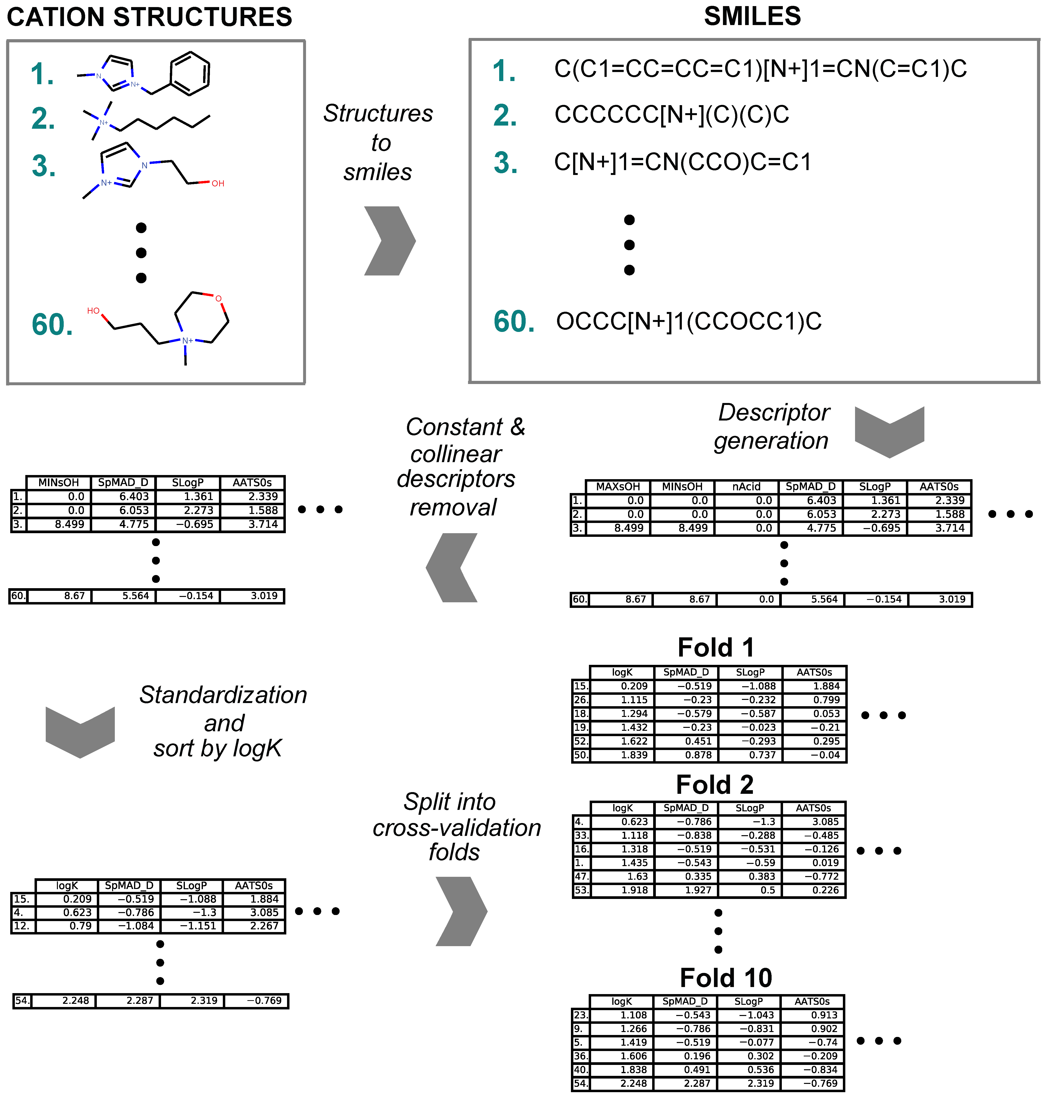
4.2. Cation Structure and Data Series Preparation Workflow

The preparation of each data series for modeling followed a general workflow (summarized in Figure 7) that consisted of SMILES [110] creation for the cation part of the ionic liquid, descriptor generation, removal of redundant descriptors, standardization of descriptor values and subdividing for cross-validation. The names of the cations were used to create the corresponding SMILES representations. The molecular descriptors were calculated with the Mordred [71] library (version 1.1.1) that uses the rdkit [111] library (version 2018.09.3). The calculation resulted in 1613 2D molecular descriptors for each cation, which formed a cation-descriptor matrix. The redundant constant value descriptors and all but one in sets of collinear descriptors were removed from the solutes cation-descriptor matrix. The remaining descriptors were standardized to a mean of 0 and a standard deviation of 1. In the resulting matrices, the cations were sorted in the ascending order by log K values. Then, the cations were subdivided into ten folds where each fold consisted of every tenth cation in the log K sorted matrix. The described partitioning scheme resulted in ten data sets that contained evenly distributed partition coefficient values for 10-fold cross-validation. As a result of the preparation, three cation-descriptor matrices for benzene, hexane and cyclohexane all consisted of 1180 descriptors and 10-folds.

4.3. Multiple Linear Regression

Multiple linear regression (MLR) is given by the linear combination of molecular descriptors with a modeled property $\widehat{y}$ [112]:

$$\widehat{y}={\beta }_0+{\beta }_1{X}_1+{\beta }_2{X}_2+\dots +{\beta }_k{X}_k,$$

(5)

where β₀, β₁, …, β_k are regression coefficients and X₁, X₂, …, X_k are molecular descriptors. The regression coefficients vector $\widehat{\beta }$ is regularly calculated using the ordinary least squares method to minimize squared error [112]:

$$\widehat{\beta }={(X^{T}X)}^{-1}{X}^{T}y,$$

(6)

given experimental property values y and the molecular descriptor values of matrix X.

The orthogonal matching pursuit (OMP) algorithm is a bottom-up feature selection algorithm that selects a feature into a linear model on each iteration based on the correlation of the features to the residual of the linear model estimations [48,113]. OMP was used for the selection of features (molecular descriptors) into MLR models. The OMP algorithm is computationally efficient for the selection of descriptors that have a low correlation between each other and therefore accounts for potentially more varied chemical information with each selected descriptor. From the Scikit-learn [114] (version 0.24.2) library, the OrthogonalMatchingPursuit class was used as the implementation of OMP.

The expansion of the search space of the OMP algorithm and improvements in the selected combination of descriptors was achieved by iteratively expelling the highest correlated descriptor to log K. In order to procure a wider selection of linear models using OMP, after the initial selection, the descriptor with the highest correlation to log K was expelled and OMP was applied again. This process was repeated until the highest correlation to log K complied with R < 0.4. Out of the models with the same number of descriptors found by the OMP algorithm, the one with the highest coefficient of determination was deemed optimal. The number of descriptors selected started with one and the amount was incremented until the model did not show significant improvement. In this case, significant improvement was confirmed if the parameter with an extra descriptor corrected at least 20% of the prediction error according to the coefficient of determination.

4.4. Support Vector Regression

The support vector regression (SVR) algorithm solves a constrained optimization problem to find the optimal set of training points x_sv called the support vectors, the regression coefficients, and the intercept in the SVR model [115]. The support vectors are equidistant from the computed regression line and mark the margin boundary termed the ε-tube around the regression line, where points outside the ε-tube are penalized in the optimization expression.

The resulting model can account for non-linearity with respect to the features due to transformations via the kernel function [116]. The kernel function maps training points into higher dimensional space, which characterizes the similarity between two data points and can be chosen according to the modeling problem. The linear, polynomial, radial basis function (RBF) and sigmoid kernel are some of the commonly applied kernel functions. The SVR algorithm involves hyperparameters C and ε, which influence the optimization expression. The error penalization term C is generally chosen to be 1 but its value should be configured with attention to the input data, as it influences how much the errors $\sigma$_i penalize the optimization expression and in turn deviate the regression line. In addition to C and ε, the chosen kernel function may contain additional hyperparameters; for example, the RBF function can be tuned by changing a scale coefficient γ.

The Scikit-learn [114] (version 0.24.2) library SVR class and the RBF kernel were used as SVR implementation. The prediction of the SVR model for a molecule with descriptors $x$ is as follows:

$$\widehat{y}={{\displaystyle \sum }}_{i\in SV}{\alpha }_i K\left(x_i,x\right)+b,$$

(7)

where $\alpha$ are the regression coefficients of the support vector training points, $x_i$ includes descriptor values for the i-th support vector, K is the kernel function, and b is the intercept.

Descriptor selection for the SVR models followed a bottom-up scheme, where descriptors were selected into the model based on the highest 10-fold cross-validated validation coefficient of determination. After a new descriptor was selected into the model, all descriptors were also substituted one by one until the model did not improve anymore from any single parameter substitution. The concluded optimal model had its hyperparameters C, ε and γ tuned by refitting with a combination of hyperparameters from a grid of predetermined values (

Table 6. SVR hyperparameter tuning values.

C	0.001, 0.005, 0.1, 0.5, 1,5, 10, 50, 100, 500, 1000
ε	0.001, 0.005, 0.01, 0.05, 0.1, 0.5, 1.0, 5.0, 10.0
γ	0.001, 0.005, 0.01, 0.05, 0.1, ‘auto’, ‘scale’

). Whether a higher parameter model was considered better was based on improvement in comparison to the optimal model with one less parameter. If the higher parameter model corrected at least 20% of the prediction error, more parameters were added until the model did not improve by 20% anymore.

4.5. Gaussian Process Regression

In the Gaussian process regression (GPR) method, a distribution over functions is defined using the training data, a covariance function and corresponding log K values [117]. The predictions from the fitted GPR model form a full predictive distribution with a mean and standard deviation at every point of the input space [117]. The GPR model predicted distribution for validation data points $x_{*i}$ can be calculated by evaluating the mean ${\overline{f}}_{*}$ and the covariance matrix $V\left[f_{*}\right]$ from the following [117]:

$${\overline{f}}_{*}=K\left(X_{*},X\right){[K\left(X,X\right)]}^{-1}y,$$

(8)

$$V\left[f_{*}\right]=K\left(X_{*},X_{*}\right)-K\left(X_{*},X\right){[K\left(X,X\right)]}^{-1}K\left(X,X_{*}\right),$$

(9)

where $X$ is the training cation-descriptor matrix, $X_{*}$ is the validation cation-descriptor matrix, $y$ is the vector of log K values corresponding to the training data points, and K(A, B) is the kernel dot product, e.g., the covariance function between the input matrices A and B [117]. The commonly used RBF kernel function maps the descriptors into an infinite-dimensional descriptor space; however, by only using dot products between kernel mapped inputs, the individual kernel-mapped descriptors do not need to be calculated [117].

Kernels used in constructing the GPR model have an effect on the derived space of functions [117]. Commonly applied kernels include the constant, white noise, dot product, polynomial, RBF kernel and combinations [117]. In this study, the Scikit-learn [118] (version 0.24.2) library implementation of the GaussianProcessRegressor class was used with the kernel combination of the sum of WhiteKernel, DotProduct and the RBF kernel from the same library module. The fitting of the GaussianProcessRegressor also optimized the kernel’s hyperparameters [118]. Of the GPR models with the same number of descriptors, the model with the highest coefficient of determination was considered optimal. Whether a higher parameter model was better than a model with one less parameter was based on a 20% error improvement, similarly to the SVR descriptor selection method.

4.6. Diagnostics and Applicability Domain of Models

The performance of models was evaluated using 10-fold cross-validation to avoid overfitting. The model predictive capability was assessed in the training process by calculating the coefficient of determination (Equation (10)), $r^2$, and evaluation external to descriptor selection and producing the models was measured by the concordance correlation coefficient (Equation (11)) [119], CCC. As another comparison tool, the mean squared error (Equation (12)), RMSE, has been provided along with the models’ statistical parameters.

$$r^2=1-\frac{\sum {(y_i-{\widehat{y}}_i)}^2}{\sum {(y_i-{\stackrel{-}{y}}_i)}^2},$$

(10)

$$CCC=\frac{2{{\displaystyle \sum }}_{i=1}^n\left({\widehat{y}}_i-\stackrel{-}{\widehat{y}}\right){\left(y_i-\stackrel{-}{y}\right)}_{}}{{{\displaystyle \sum }}_{i=1}^n{({\widehat{y}}_i-\stackrel{-}{\widehat{y}})}^2+{{\displaystyle \sum }}_{i=1}^n{(y_i-\stackrel{-}{y})}^2+n{(\stackrel{-}{\widehat{y}}-\widehat{y})}^2},$$

(11)

$$RMSE=\sqrt{\frac{1}{n}\sum {(y_i-{\widehat{y}}_i)}^2}$$

(12)

Additional diagnostics were performed for the linear models to identify outliers, high leverage data points, and influential data points. Data points exceeding the critical leverage value $h^{*}{}_3$ (Equation (14)) are considered as high leverage, where the critical value is calculated from the model’s descriptor amount $k$ and data set size $n$. A matrix of model molecular descriptor values in columns along with an additional constant column comprises design matrix $X$ used in the calculation of the leverage $h_{ii}$ of a data point $i$:

$$H=X·{(X^T·X)}^{-1}·X^T,$$

(13)

$$h^{*}{}_3=\frac{3·\left(k+1\right)}{n},$$

(14)

where H is called the hat matrix and $h_{ii}$ includes its main diagonal values. For outlier diagnostics, the standardized residuals $r_i$ of the model are examined for each data point $i$:

$$r_i=\frac{{\widehat{y}}_i-y_i}{\widehat{\sigma }·\sqrt{1-h_{ii}}},$$

(15)

$${\widehat{\sigma }}^2=\frac{e^T·e}{n-k-1},$$

(16)

$$e_i=\left(1-h_{ii}\right)·y_i,$$

(17)

where $\widehat{\sigma }$ is the mean squared error of the linear regression model, and $e_i$ is the residual of the $i$-th data point. A data point with $\left|r_i\right|>2$ should be inspected and a data point with $\left|r_i\right|>3$ is likely to be an outlier and requires closer analysis.

An observation’s influence on the model is assessed by Cook’s distance (D_i), a measure of the effect of removing a given data point.

$$D_i=\frac{r_i{}^2}{k+1}·\frac{h_{ii}}{1-h_{ii}}$$

(18)

A common rule is to take a closer look at observations with Cook’s distance higher than one. The accuracy of the model’s predictions may be distorted by high leverage and/or high residual observations and Cook’s distance provides a method to find influential data points that could indicate the regions of the molecular space, where more experimental data are required.

4.7. Availability of Regression Models

The MLR, SVR and GPR models and related data can be made available in various data formats [120]. To follow the best practices of QSAR model reporting [121], the models with data are stored at the QsarDB repository [122] in QSAR Data Bank format [123]. A digital object identifier (DOI) has been assigned for the models and data [124].

5. Conclusions

The present study successfully tested the hypothesis that the gas-ionic liquid partition coefficient (log K) can be successfully modeled in a data-driven manner based on the partial structure of the ionic liquid, namely the varying cationic counterpart. QSPR models were derived for gas-ionic liquid partition coefficients for three organic compounds hexane, cyclohexane and benzene in the series of ionic liquids with common bis(trifluoromethylsulfonyl)imide ([Tf2N]⁻) anion using linear and non-linear QSPR methods. Variation in ionic counterpart makes it possible to more specifically understand the molecular interactions of partitioning by the ionic liquid and how to enable finding the application-appropriate ionic liquid. Three machine learning approaches (MLR, SVR and GPR) were used to derive data driven models and their performance was compared. The comparison of different modeling methods showed that both linear and non-linear models have excellent performance, while non-linear models had better performance. The selection of a suitable model for the prediction of log K depends on the circumstances and they offer different benefits. For example, the MLR models have an advantage in that they are simple and easy to interpret. The SVM models had the best prediction performance, and GPR models can provide uncertainty measurements on the predictions. The cross-validation coefficients of determination were in the range of 0.71–0.93 and also other performance statistics indicated strong accuracy of models for all data series and machine learning methods. The analysis and interpretation of descriptors revealed how the structure of cationic counterpart influences molecular interactions and that generally higher lipophilicity and dispersion interaction capability and lower polarity in the cations induces a higher partition coefficient for benzene, hexane, cyclohexane and hydrocarbons in general. Applicability domain analysis of models exposed outliers, but it concluded that they are not highly influential and that the models are applicable to a wide selection of cation families with variable size, polarity and aliphatic or aromatic nature.

References

1. MacFarlane, D.R.; Kar, M.; Pringle, J.M. An Introduction to Ionic Liquids. In Fundamentals of Ionic Liquids; John Wiley & Sons, Ltd.: Hoboken, NJ, USA, 2017; pp. 1–25. [Google Scholar] [CrossRef]
2. Hallett, J.P.; Welton, T. Room-Temperature Ionic Liquids: Solvents for Synthesis and Catalysis. 2. Chem. Rev. 2011, 111, 3508–3576. [Google Scholar] [CrossRef] [PubMed]
3. Wasserscheid, P.; Welton, T. (Eds.) Ionic Liquids in Synthesis, 2nd ed; John Wiley & Sons, Ltd.: Hoboken, NJ, USA, 2007; Volume 1. [Google Scholar]
4. MacFarlane, D.R.; Kar, M.; Pringle, J.M. Solvent Properties of Ionic Liquids: Applications in Synthesis and Separations. In Fundamentals of Ionic Liquids; John Wiley & Sons, Ltd.: Hoboken, NJ, USA, 2017; pp. 149–176. [Google Scholar] [CrossRef]
5. Pârvulescu, V.I.; Hardacre, C. Catalysis in Ionic Liquids. Chem. Rev. 2007, 107, 2615–2665. [Google Scholar] [CrossRef] [PubMed]
6. Steinrück, H.-P.; Wasserscheid, P. Ionic Liquids in Catalysis. Catal. Lett. 2015, 145, 380–397. [Google Scholar] [CrossRef]
7. Benavente, J.; Rodríguez-Castellón, E. Application of Electrochemical Impedance Spectroscopy (EIS) and X-ray Photoelectron Spectroscopy (XPS) to the Characterization of RTILs for Electrochemical Applications. In Ionic Liquids: Applications and Perspectives; InTech: London, UK, 2011; pp. 607–626. [Google Scholar] [CrossRef] [Green Version]
8. Liu, Y.-S.; Pan, G.-B. Ionic Liquids for the Future Electrochemical Applications. In Ionic Liquids: Applications and Perspectives; InTech: London, UK, 2011; pp. 627–642. [Google Scholar] [CrossRef] [Green Version]
9. Faridbod, F.; Ganjali, M.R.; Norouzi, P.; Riahi, S.; Rashedi, H. Application of Room Temperature Ionic Liquids in Electrochemical Sensors and Biosensors. In Ionic Liquids: Applications and Perspectives; InTech: London, UK, 2011; pp. 643–658. [Google Scholar] [CrossRef] [Green Version]
10. Ikeda, Y.; Asanuma, N.; Ohashi, Y. Electrochemical Studies on Uranyl(VI) Chloride Complexes in 1-Butyl-3-Methyl- Imidazolium Based Ionic Liquids and Their Application to Pyro-Reprocessing and Treatment of Wastes Contaminated with Uranium. In Ionic Liquids: Applications and Perspectives; InTech: London, UK, 2011; pp. 659–674. [Google Scholar] [CrossRef] [Green Version]
11. Singh, V.V.; Anil, K. Nigam; Anirudh Batra; Mannan Boopathi; Beer Singh; Rajagopalan Vijayaraghavan. Applications of Ionic Liquids in Electrochemical Sensors and Biosensors. Int. J. Electrochem. 2012, 2012, 165683. [Google Scholar] [CrossRef] [Green Version]
12. Angel, A.J. Torriero. Electrochemistry in Ionic Liquids, 1st ed.; Springer International Publishing: Berlin/Heidelberg, Germany, 2015; Volume 1. [Google Scholar]
13. MacFarlane, D.R.; Kar, M.; Pringle, J.M. Electrochemistry of and in Ionic Liquids. In Fundamentals of Ionic Liquids; John Wiley & Sons, Ltd.: Hoboken, NJ, USA, 2017; pp. 177–207. [Google Scholar] [CrossRef]
14. MacFarlane, D.R.; Kar, M.; Pringle, J.M. Electrochemical Device Applications. In Fundamentals of Ionic Liquids; John Wiley & Sons, Ltd.: Hoboken, NJ, USA, 2017; pp. 209–230. [Google Scholar] [CrossRef]
15. Bogdanov, M.; Bogdanov, M. Ionic Liquids as Alternative Solvents for Extraction of Natural Products; Springer: Berlin/Heidelberg, Germany, 2014; pp. 127–166. [Google Scholar] [CrossRef]
16. Tang, B.; Bi, W.; Tian, M.; Row, K.H. Application of Ionic Liquid for Extraction and Separation of Bioactive Compounds from Plants. J. Chromatogr. B 2012, 904, 1–21. [Google Scholar] [CrossRef]
17. Ventura, S.P.M.; e Silva, F.A.; Quental, M.V.; Mondal, D.; Freire, M.G.; Coutinho, J.A.P. Ionic-Liquid-Mediated Extraction and Separation Processes for Bioactive Compounds: Past, Present, and Future Trends. Chem. Rev. 2017, 117, 6984–7052. [Google Scholar] [CrossRef]
18. Xiao, J.; Chen, G.; Li, N. Ionic Liquid Solutions as a Green Tool for the Extraction and Isolation of Natural Products. Molecules 2018, 23, 1765. [Google Scholar] [CrossRef] [Green Version]
19. Berthod, A.; Ruiz-Ángel, M.J.; Carda-Broch, S. Ionic Liquids in Separation Techniques. J. Chromatogr. A 2008, 1184, 6–18. [Google Scholar] [CrossRef]
20. Berthod, A.; Ruiz-Ángel, M.J.; Carda-Broch, S. Recent Advances on Ionic Liquid Uses in Separation Techniques. J. Chromatogr. A 2018, 1559, 2–16. [Google Scholar] [CrossRef]
21. Flieger, J.; Blicharska, E.; Czajkowska, A. Ionic Liquids as Solvents in Separation Processes. Austin. J. Anal. Pharm. Chem 2014, 1, 1009. [Google Scholar]
22. Kokorin, A. Ionic Liquids: Applications and Perspectives; InTech: Rijeka, Croatia; Shanghai, China, 2011. [Google Scholar] [CrossRef]
23. Marrucho, I.; Branco, L.; Rebelo, L.P.N. Ionic Liquids in Pharmaceutical Applications. Annu. Rev. Chem. Biomol. Eng. 2014, 5, 527–546. [Google Scholar] [CrossRef] [PubMed]
24. Javed, F.; Ullah, F.; Zakaria, M.R.; Akil, H.M. An Approach to Classification and Hi-Tech Applications of Room-Temperature Ionic Liquids (RTILs): A Review. J. Mol. Liq. 2018, 271, 403–420. [Google Scholar] [CrossRef]
25. Anderson, J.L.; Clark, K.D. Ionic Liquids as Tunable Materials in (Bio)Analytical Chemistry. Anal. Bioanal. Chem. 2018, 410, 4565–4566. [Google Scholar] [CrossRef] [PubMed] [Green Version]
26. Itoh, T.; Koo, Y.-M. (Eds.) Application of Ionic Liquids in Biotechnology; Advances in Biochemical Engineering/Biotechnology; Springer International Publishing: Berlin/Heidelberg, Germany, 2019. [Google Scholar] [CrossRef]
27. Mohammadi-Jam, S.; Waters, K.E. Inverse Gas Chromatography Applications: A Review. Adv. Colloid Interface Sci. 2014, 212, 21–44. [Google Scholar] [CrossRef]
28. Paduszyński, K.; Domańska, U. Limiting Activity Coefficients and Gas–Liquid Partition Coefficients of Various Solutes in Piperidinium Ionic Liquids: Measurements and LSER Calculations. J. Phys. Chem. B 2011, 115, 8207–8215. [Google Scholar] [CrossRef]
29. Koel, M. Ionic Liquids in Chemical Analysis. Crit. Rev. Anal. Chem. 2005, 35, 177–192. [Google Scholar] [CrossRef]
30. Zhao, H.; Baker, G.A.; Wagle, D.V.; Ravula, S.; Zhang, Q. Tuning Task-Specific Ionic Liquids for the Extractive Desulfurization of Liquid Fuel. ACS Sustain. Chem. Eng. 2016, 4, 4771–4780. [Google Scholar] [CrossRef]
31. Tian, J.; Fu, S.; Zhang, C.; Lucia, L. Tuning Solute Partitioning Coefficients in a Biphasic Ionic Liquid/Water System to Facilitate Extraction of Lignin-Oxidized Aromatics. BioResources 2015, 10, 4099–4109. [Google Scholar] [CrossRef] [Green Version]
32. Marcilla, R.; Blazquez, J.A.; Rodriguez, J.; Pomposo, J.A.; Mecerreyes, D. Tuning the Solubility of Polymerized Ionic Liquids by Simple Anion-Exchange Reactions. J. Polym. Sci. Part Polym. Chem. 2004, 42, 208–212. [Google Scholar] [CrossRef]
33. Florindo, C.; Araújo, J.M.M.; Alves, F.; Matos, C.; Ferraz, R.; Prudêncio, C.; Noronha, J.P.; Petrovski, Ž.; Branco, L.; Rebelo, L.P.N.; et al. Evaluation of Solubility and Partition Properties of Ampicillin-Based Ionic Liquids. Int. J. Pharm. 2013, 456, 553–559. [Google Scholar] [CrossRef] [Green Version]
34. Speight, J.G. Molecular Interactions, Partitioning, and Thermodynamics. In Reaction Mechanisms in Environmental Engineering; Elsevier: Amsterdam, The Netherlands, 2018; pp. 307–336. [Google Scholar] [CrossRef]
35. Abraham, M.H. Scales of Solute Hydrogen-Bonding: Their Construction and Application to Physicochemical and Biochemical Processes. Chem. Soc. Rev. 1993, 22, 73. [Google Scholar] [CrossRef]
36. Anderson, J.L.; Ding, J.; Welton, T.; Armstrong, D.W. Characterizing Ionic Liquids On the Basis of Multiple Solvation Interactions. J. Am. Chem. Soc. 2002, 124, 14247–14254. [Google Scholar] [CrossRef] [PubMed] [Green Version]
37. Anderson, J.L.; Armstrong, D.W. High-Stability Ionic Liquids. A New Class of Stationary Phases for Gas Chromatography. Anal. Chem. 2003, 75, 4851–4858. [Google Scholar] [CrossRef] [PubMed] [Green Version]
38. Anderson, J.L.; Armstrong, D.W. Immobilized Ionic Liquids as High-Selectivity/High-Temperature/High-Stability Gas Chromatography Stationary Phases. Anal. Chem. 2005, 77, 6453–6462. [Google Scholar] [CrossRef] [PubMed] [Green Version]
39. Abraham, M.H.; Acree, W.E. Comparative Analysis of Solvation and Selectivity in Room Temperature Ionic Liquids Using the Abraham Linear Free Energy Relationship. Green Chem. 2006, 8, 906–915. [Google Scholar] [CrossRef]
40. Acree, W.E.; Abraham, M.H. The Analysis of Solvation in Ionic Liquids and Organic Solvents Using the Abraham Linear Free Energy Relationship. J. Chem. Technol. Biotechnol. 2006, 81, 1441–1446. [Google Scholar] [CrossRef]
41. Revelli, A.-L.; Mutelet, F.; Jaubert, J.-N. Prediction of Partition Coefficients of Organic Compounds in Ionic Liquids: Use of a Linear Solvation Energy Relationship with Parameters Calculated through a Group Contribution Method. Ind. Eng. Chem. Res. 2010, 49, 3883–3892. [Google Scholar] [CrossRef]
42. Yue, D.; Acree, W.E.; Abraham, M.H. Development of Abraham Model IL-Specific Correlations for N-Triethyl(Octyl)Ammonium Bis(Fluorosulfonyl)Imide and 1-Butyl-3-Methylpyrrolidinium Bis(Fluorosulfonyl)Imide. Phys. Chem. Liq. 2018, 57, 733–745. [Google Scholar] [CrossRef]
43. Mutelet, F.; Baker, G.A.; Zhao, H.; Churchill, B.; Acree, W.E. Development of Abraham Model Correlations for Short-Chain Glycol-Grafted Imidazolium and Pyridinium Ionic Liquids from Inverse Gas-Chromatographic Measurements. J. Mol. Liq. 2020, 317, 113983. [Google Scholar] [CrossRef]
44. Churchill, B.; Casillas, T.; Acree, W.E.; Abraham, M.H. Abraham Solvation Parameter Model: Calculation of Ion-Specific Equation Coefficients for the N-Ethyl-N-Methylmorpholinium and N-Octyl-N-Methylmorpholinium Cations. Phys. Chem. Liq. 2020, 59, 575–584. [Google Scholar] [CrossRef]
45. Sprunger, L.; Clark, M.; Acree, W.E.; Abraham, M.H. Characterization of Room-Temperature Ionic Liquids by the Abraham Model with Cation-Specific and Anion-Specific Equation Coefficients. J. Chem. Inf. Model. 2007, 47, 1123–1129. [Google Scholar] [CrossRef] [PubMed]
46. Katritzky, A.R.; Kuanar, M.; Stoyanova-Slavova, I.B.; Slavov, S.H.; Dobchev, D.A.; Karelson, M.; Acree, W.E. Quantitative Structure–Property Relationship Studies on Ostwald Solubility and Partition Coefficients of Organic Solutes in Ionic Liquids. J. Chem. Eng. Data 2008, 53, 1085–1092. [Google Scholar] [CrossRef]
47. Khooshechin, S.; Dashtbozorgi, Z.; Golmohammadi, H.; Acree, W.E. QSPR Prediction of Gas-to-Ionic Liquid Partition Coefficient of Organic Solutes Dissolved in 1-(2-Hydroxyethyl)-1-Methylimidazolium Tris(Pentafluoroethyl)Trifluorophosphate Using the Replacement Method and Support Vector Regression. J. Mol. Liq. 2014, 196, 43–51. [Google Scholar] [CrossRef]
48. Toots, K.M.; Sild, S.; Leis, J.; Acree, W.E.; Maran, U. The Quantitative Structure-Property Relationships for the Gas-Ionic Liquid Partition Coefficient of a Large Variety of Organic Compounds in Three Ionic Liquids. J. Mol. Liq. 2021, 343, 117573. [Google Scholar] [CrossRef]
49. Katritzky, A.R.; Oliferenko, A.A.; Oliferenko, P.V.; Petrukhin, R.; Tatham, D.B.; Maran, U.; Lomaka, A.; Acree, W.E. A General Treatment of Solubility. 1. The QSPR Correlation of Solvation Free Energies of Single Solutes in Series of Solvents. J. Chem. Inf. Comput. Sci. 2003, 43, 1794–1805. [Google Scholar] [CrossRef] [PubMed]
50. Katritzky, A.R.; Oliferenko, A.A.; Oliferenko, P.V.; Petrukhin, R.; Tatham, D.B.; Maran, U.; Lomaka, A.; Acree, W.E. A General Treatment of Solubility. 2. QSPR Prediction of Free Energies of Solvation of Specified Solutes in Ranges of Solvents. J. Chem. Inf. Comput. Sci. 2003, 43, 1806–1814. [Google Scholar] [CrossRef] [PubMed]
51. Katritzky, A.R.; Tulp, I.; Fara, D.C.; Lauria, A.; Maran, U.; Acree, W.E. A General Treatment of Solubility. 3. Principal Component Analysis (PCA) of the Solubilities of Diverse Solutes in Diverse Solvents. J. Chem. Inf. Model. 2005, 45, 913–923. [Google Scholar] [CrossRef]
52. Tulp, I.; Dobchev, D.A.; Katritzky, A.R.; Acree, W.E.; Maran, U. A General Treatment of Solubility 4. Description and Analysis of a PCA Model for Ostwald Solubility Coefficients. J. Chem. Inf. Model. 2010, 50, 1275–1283. [Google Scholar] [CrossRef] [Green Version]
53. Katritzky, A.R.; Tatham, D.B.; Maran, U. Correlation of the Solubilities of Gases and Vapors in Methanol and Ethanol with Their Molecular Structures. J. Chem. Inf. Comput. Sci. 2001, 41, 358–363. [Google Scholar] [CrossRef]
54. Katritzky, A.R.; Maran, U.; Karelson, M.; Lobanov, V.S. Prediction of Melting Points for the Substituted Benzenes: A QSPR Approach. J. Chem. Inf. Comput. Sci. 1997, 37, 913–919. [Google Scholar] [CrossRef]
55. Viira, B.; García-Sosa, A.T.; Maran, U. Chemical Structure and Correlation Analysis of HIV-1 NNRT and NRT Inhibitors and Database-Curated, Published Inhibition Constants with Chemical Structure in Diverse Datasets. J. Mol. Graph. Model. 2017, 76, 205–223. [Google Scholar] [CrossRef] [PubMed]
56. Moosus, M.; Maran, U. Quantitative Structure–Activity Relationship Analysis of Acute Toxicity of Diverse Chemicals to Daphnia Magna with Whole Molecule Descriptors. SAR QSAR Environ. Res. 2011, 22, 757–774. [Google Scholar] [CrossRef] [PubMed]
57. Aruoja, V.; Moosus, M.; Kahru, A.; Sihtmäe, M.; Maran, U. Measurement of Baseline Toxicity and QSAR Analysis of 50 Non-Polar and 58 Polar Narcotic Chemicals for the Alga Pseudokirchneriella Subcapitata. Chemosphere 2014, 96, 23–32. [Google Scholar] [CrossRef] [PubMed]
58. Piir, G.; Sild, S.; Maran, U. Classifying Bio-Concentration Factor with Random Forest Algorithm, Influence of the Bio-Accumulative vs. Non-Bio-Accumulative Compound Ratio to Modelling Result, and Applicability Domain for Random Forest Model. SAR QSAR Environ. Res. 2014, 25, 967–981. [Google Scholar] [CrossRef]
59. Oja, M.; Sild, S.; Maran, U. Logistic Classification Models for PH–Permeability Profile: Predicting Permeability Classes for the Biopharmaceutical Classification System. J. Chem. Inf. Model. 2019, 59, 2442–2455. [Google Scholar] [CrossRef]
60. Piir, G.; Sild, S.; Maran, U. Binary and Multi-Class Classification for Androgen Receptor Agonists, Antagonists and Binders. Chemosphere 2021, 262, 128313. [Google Scholar] [CrossRef]
61. Käärik, M.; Maran, U.; Arulepp, M.; Perkson, A.; Leis, J. Quantitative Nano-Structure–Property Relationships for the Nanoporous Carbon: Predicting the Performance of Energy Storage Materials. ACS Appl. Energy Mater. 2018, 1, 4016–4024. [Google Scholar] [CrossRef]
62. Käärik, M.; Arulepp, M.; Käärik, M.; Maran, U.; Leis, J. Characterization and Prediction of Double-Layer Capacitance of Nanoporous Carbon Materials Using the Quantitative Nano-Structure-Property Relationship Approach Based on Experimentally Determined Porosity Descriptors. Carbon 2020, 158, 494–504. [Google Scholar] [CrossRef]
63. Mohsenipour, A.; Mozaffarian, M.; Pazuki, G.; Naji, L. Fabrication of High Performance Supercapacitors Based on Ethyl Methyl Imidazolium Bis(Trifluoromethylsulfonyl) Imide (EMIMTFSI)-Decorated Reduced Graphene Oxide (RGO). J. Alloys Compd. 2022, 892, 162093. [Google Scholar] [CrossRef]
64. Gollakota, A.R.K.; Subbaiah Munagapati, V.; Shu, C.-M.; Wen, J.-C. Adsorption of Cr (VI), and Pb (II) from Aqueous Solution by 1-Butyl-3-Methylimidazolium Bis(Trifluoromethylsulfonyl)Imide Functionalized Biomass Hazel Sterculia (Sterculia foetida L.). J. Mol. Liq. 2022, 350, 118534. [Google Scholar] [CrossRef]
65. Kuczak, M.; Musial, M.; Malarz, K.; Rurka, P.; Zorebski, E.; Musiol, R.; Dzida, M.; Mrozek-Wilczkiewicz, A. Anticancer Potential and through Study of the Cytotoxicity Mechanism of Ionic Liquids That Are Based on the Trifluoromethanesulfonate and Bis (Trifluoromethylsulfonyl)Imide Anions. J. Hazard. Mater. 2022, 427, 128160. [Google Scholar] [CrossRef] [PubMed]
66. Doblinger, S.; Silvester, D.S.; Costa Gomes, M. Functionalized Imidazolium Bis(Trifluoromethylsulfonyl)Imide Ionic Liquids for Gas Sensors: Solubility of H2, O2 and SO2. Fluid Phase Equilibria 2021, 549, 113211. [Google Scholar] [CrossRef]
67. Gano, M.; Klebeko, J.; Pełech, R. Efficient Esterification of Curcumin in Bis(Trifluoromethylsulfonyl)Imide-Based Ionic Liquids. J. Mol. Liq. 2021, 337, 116420. [Google Scholar] [CrossRef]
68. Zabihpour, T.; Shahidi, S.-A.; Karimi-Maleh, H.; Ghorbani-HasanSaraei, A. An Ultrasensitive Electroanalytical Sensor Based on MgO/SWCNTs- 1-Butyl-3-Methylimidazolium Bis(Trifluoromethylsulfonyl)Imide Paste Electrode for the Determination of Ferulic Acid in the Presence Sulfite in Food Samples. Microchem. J. 2020, 154, 104572. [Google Scholar] [CrossRef]
69. Ayuso, M.; Ovejero-Pérez, A.; Delgado-Mellado, N.; Navarro, P.; Larriba, M.; García, J.; Rodríguez, F. Tetrathiocyanatocobaltate and Bis(Trifluoromethylsulfonyl)Imide-Based Ionic Liquids as Mass Agents in the Separation of Cyclohexane and Cyclohexene Mixtures by Homogeneous Extractive Distillation. J. Chem. Thermodyn. 2021, 157, 106403. [Google Scholar] [CrossRef]
70. Hall, L.H.; Kier, L.B. Electrotopological State Indices for Atom Types: A Novel Combination of Electronic, Topological, and Valence State Information. J. Chem. Inf. Model. 1995, 35, 1039–1045. [Google Scholar] [CrossRef]
71. Moriwaki, H.; Tian, Y.-S.; Kawashita, N.; Takagi, T. Mordred: A Molecular Descriptor Calculator. J. Cheminform. 2018, 10, 4. [Google Scholar] [CrossRef] [Green Version]
72. Allred, A.L.; Rochow, E.G. A Scale of Electronegativity Based on Electrostatic Force. J. Inorg. Nucl. Chem. 1958, 5, 264–268. [Google Scholar] [CrossRef]
73. Domańska, U.; Papis, P.; Szydłowski, J. Thermodynamics and Activity Coefficients at Infinite Dilution for Organic Solutes, Water and Diols in the Ionic Liquid Choline Bis(Trifluoromethylsulfonyl)Imide. J. Chem. Thermodyn. 2014, 77, 63–70. [Google Scholar] [CrossRef]
74. Mutelet, F.; Alonso, D.; Ravula, S.; Baker, G.A.; Jiang, B.; Acree, W.E. Infinite Dilution Activity Coefficients of Solutes Dissolved in Anhydrous Alkyl(Dimethyl)Isopropylammonium Bis(Trifluoromethylsulfonyl)Imide Ionic Liquids Containing Functionalized- and Nonfunctionalized-Alkyl Chains. J. Mol. Liq. 2016, 222, 295–312. [Google Scholar] [CrossRef]
75. Revelli, A.-L.; Mutelet, F.; Jaubert, J.-N.; Garcia-Martinez, M.; Sprunger, L.M.; Acree, W.E.; Baker, G.A. Study of Ether-, Alcohol-, or Cyano-Functionalized Ionic Liquids Using Inverse Gas Chromatography. J. Chem. Eng. Data 2010, 55, 2434–2443. [Google Scholar] [CrossRef] [Green Version]
76. Moïse, J.-C.; Mutelet, F.; Jaubert, J.-N.; Grubbs, L.M.; Acree, W.E.; Baker, G.A. Activity Coefficients at Infinite Dilution of Organic Compounds in Four New Imidazolium-Based Ionic Liquids. J. Chem. Eng. Data 2011, 56, 3106–3114. [Google Scholar] [CrossRef]
77. Mutelet, F.; Revelli, A.-L.; Jaubert, J.-N.; Sprunger, L.M.; Acree, W.E.; Baker, G.A. Partition Coefficients of Organic Compounds in New Imidazolium and Tetralkylammonium Based Ionic Liquids Using Inverse Gas Chromatography. J. Chem. Eng. Data 2010, 55, 234–242. [Google Scholar] [CrossRef] [Green Version]
78. Acree, W.E.; Baker, G.A.; Mutelet, F.; Moise, J.-C. Partition Coefficients of Organic Compounds in Four New Tetraalkylammonium Bis(Trifluoromethylsulfonyl)Imide Ionic Liquids Using Inverse Gas Chromatography. J. Chem. Eng. Data 2011, 56, 3688–3697. [Google Scholar] [CrossRef] [Green Version]
79. Revelli, A.-L.; Sprunger, L.M.; Gibbs, J.; Acree, W.E.; Baker, G.A.; Mutelet, F. Activity Coefficients at Infinite Dilution of Organic Compounds in Trihexyl(Tetradecyl)Phosphonium Bis(Trifluoromethylsulfonyl)Imide Using Inverse Gas Chromatography. J. Chem. Eng. Data 2009, 54, 977–985. [Google Scholar] [CrossRef]
80. Mutelet, F.; Hassan, E.-S.R.E.; Stephens, T.W.; Acree, W.E.; Baker, G.A. Activity Coefficients at Infinite Dilution for Organic Solutes Dissolved in Three 1-Alkyl-1-Methylpyrrolidinium Bis(Trifluoromethylsulfonyl)Imide Ionic Liquids Bearing Short Linear Alkyl Side Chains of Three to Five Carbons. J. Chem. Eng. Data 2013, 58, 2210–2218. [Google Scholar] [CrossRef] [Green Version]
81. Acree, W.E.; Baker, G.A.; Revelli, A.-L.; Moise, J.-C.; Mutelet, F. Activity Coefficients at Infinite Dilution for Organic Compounds Dissolved in 1-Alkyl-1-Methylpyrrolidinium Bis(Trifluoromethylsulfonyl)Imide Ionic Liquids Having Six-, Eight-, and Ten-Carbon Alkyl Chains. J. Chem. Eng. Data 2012, 57, 3510–3518. [Google Scholar] [CrossRef]
82. Grubbs, L.M.; Ye, S.; Saifullah, M.; Acree, W.E.; Twu, P.; Anderson, J.L.; Baker, G.A.; Abraham, M.H. Correlation of the Solubilizing Abilities of Hexyl(Trimethyl)Ammonium Bis((Trifluoromethyl)Sulfonyl)Imide, 1-Propyl-1-Methylpiperidinium Bis((Trifluoromethyl)Sulfonyl)Imide, and 1-Butyl-1-Methyl-Pyrrolidinium Thiocyanate. J. Solut. Chem. 2011, 40, 2000–2022. [Google Scholar] [CrossRef]
83. Ayad, A.; Mutelet, F.; Negadi, A.; Acree, W.E.; Jiang, B.; Lu, A.; Wagle, D.V.; Baker, G.A. Activity Coefficients at Infinite Dilution for Organic Solutes Dissolved in Two 1-Alkylquinuclidinium Bis(Trifluoromethylsulfonyl)Imides Bearing Alkyl Side Chains of Six and Eight Carbons. J. Mol. Liq. 2016, 215, 176–184. [Google Scholar] [CrossRef]
84. Mutelet, F.; Baker, G.A.; Ravula, S.; Qian, E.; Wang, L.; Acree, W.E. Infinite Dilution Activity Coefficients and Gas-to-Liquid Partition Coefficients of Organic Solutes Dissolved in 1-Sec-Butyl-3-Methylimidazolium Bis(Trifluoromethylsulfonyl)Imide and in 1-Tert-Butyl-3-Methylimidazolium Bis(Trifluoromethylsulfonyl)Imide. Phys. Chem. Liq. 2018, 57, 453–472. [Google Scholar] [CrossRef]
85. Mutelet, F.; Ravula, S.; Baker, G.A.; Woods, D.; Tong, X.; Acree, W.E. Infinite Dilution Activity Coefficients and Gas-to-Liquid Partition Coefficients of Organic Solutes Dissolved in 1-Benzylpyridinium Bis(Trifluoromethylsulfonyl)Imide and 1-Cyclohexylmethyl-1-Methylpyrrolidinium Bis(Trifluoromethylsulfonyl)Imide. J. Solut. Chem. 2018, 47, 308–335. [Google Scholar] [CrossRef]
86. Mutelet, F.; Djebouri, H.; Baker, G.A.; Ravula, S.; Jiang, B.; Tong, X.; Woods, D.; Acree, W.E. Study of Benzyl- or Cyclohexyl-Functionalized Ionic Liquids Using Inverse Gas Chromatography. J. Mol. Liq. 2017, 242, 550–559. [Google Scholar] [CrossRef]
87. Baelhadj, A.C.; Mutelet, F.; Jiang, B.; Acree, W.E. Activity Coefficients at Infinite Dilution for Organic Solutes Dissolved in Two 1,2,3-Tris(Diethylamino)Cyclopenylium Based Room Temperature Ionic Liquids. J. Mol. Liq. 2016, 223, 89–99. [Google Scholar] [CrossRef]
88. Domańska, U.; Marciniak, A. Activity Coefficients at Infinite Dilution Measurements for Organic Solutes and Water in the 1-Hexyloxymethyl-3-Methyl-Imidazolium and 1,3-Dihexyloxymethyl-Imidazolium Bis(Trifluoromethylsulfonyl)-Imide Ionic Liquids—The Cation Influence. Fluid Phase Equilibria 2009, 286, 154–161. [Google Scholar] [CrossRef]
89. Wlazło, M.; Karpińska, M.; Domańska, U. Thermodynamics and Selectivity of Separation Based on Activity Coefficients at Infinite Dilution of Various Solutes in 1-Allyl-3-Methylimidazolium Bis{(Trifluoromethyl)Sulfonyl}imide Ionic Liquid. J. Chem. Thermodyn. 2016, 102, 39–47. [Google Scholar] [CrossRef]
90. Domańska, U.; Wlazło, M.; Karpińska, M.; Zawadzki, M. High Selective Water/Butan-1-Ol Separation on Investigation of Limiting Activity Coefficients with [P8,8,8,8][NTf2] Ionic Liquid. Fluid Phase Equilibria 2017, 449, 1–9. [Google Scholar] [CrossRef]
91. Domańska, U.; Zawadzki, M.; Królikowska, M.; Marc Tshibangu, M.; Ramjugernath, D.; Letcher, T.M. Measurements of Activity Coefficients at Infinite Dilution of Organic Compounds and Water in Isoquinolinium-Based Ionic Liquid [C8iQuin][NTf2] Using GLC. J. Chem. Thermodyn. 2011, 43, 499–504. [Google Scholar] [CrossRef]
92. Domańska, U.; Wlazło, M. Thermodynamics and Limiting Activity Coefficients Measurements for Organic Solutes and Water in the Ionic Liquid 1-Dodecyl-3-Methylimidzolium Bis(Trifluoromethylsulfonyl) Imide. J. Chem. Thermodyn. 2016, 103, 76–85. [Google Scholar] [CrossRef]
93. Heintz, A.; Verevkin, S.P.; Ondo, D. Thermodynamic Properties of Mixtures Containing Ionic Liquids. 8. Activity Coefficients at Infinite Dilution of Hydrocarbons, Alcohols, Esters, and Aldehydes in 1-Hexyl-3-Methylimidazolium Bis(Trifluoromethylsulfonyl) Imide Using Gas−Liquid Chromatography. J. Chem. Eng. Data 2006, 51, 434–437. [Google Scholar] [CrossRef]
94. Krummen, M.; Wasserscheid, P.; Gmehling, J. Measurement of Activity Coefficients at Infinite Dilution in Ionic Liquids Using the Dilutor Technique. J. Chem. Eng. Data 2002, 47, 1411–1417. [Google Scholar] [CrossRef]
95. Królikowski, M.; Królikowska, M.; Wiśniewski, C. Separation of Aliphatic from Aromatic Hydrocarbons and Sulphur Compounds from Fuel Based on Measurements of Activity Coefficients at Infinite Dilution for Organic Solutes and Water in the Ionic Liquid N,N-Diethyl-N-Methyl-N-(2-Methoxy-Ethyl)Ammonium Bis(Trifluoromethylsulfonyl)Imide. J. Chem. Thermodyn. 2016, 103, 115–124. [Google Scholar] [CrossRef]
96. Domańska, U.; Marciniak, A. Activity Coefficients at Infinite Dilution Measurements for Organic Solutes and Water in the Ionic Liquid Triethylsulphonium Bis(Trifluoromethylsulfonyl)Imide. J. Chem. Thermodyn. 2009, 41, 754–758. [Google Scholar] [CrossRef]
97. Lu, A.; Jiang, B.; Cheeran, S.; Acree, W.E.; Abraham, M.H. Abraham Model Ion-Specific Equation Coefficients for the 1-Butyl-2,3-Dimethyimidazolium and 4-Cyano-1-Butylpyridinium Cations Calculated from Measured Gas-to-Liquid Partition Coefficient Data. Phys. Chem. Liq. 2017, 55, 218–237. [Google Scholar] [CrossRef]
98. Marciniak, A.; Wlazło, M. Activity Coefficients at Infinite Dilution and Physicochemical Properties for Organic Solutes and Water in the Ionic Liquid 1-(2-Methoxyethyl)-1-Methylpiperidinium Bis(Trifluoromethylsulfonyl)-Amide. J. Chem. Thermodyn. 2012, 49, 137–145. [Google Scholar] [CrossRef]
99. Wlazło, M.; Marciniak, A.; Zawadzki, M.; Dudkiewicz, B. Activity Coefficients at Infinite Dilution and Physicochemical Properties for Organic Solutes and Water in the Ionic Liquid 4-(3-Hydroxypropyl)-4-Methylmorpholinium Bis(Trifluoromethylsulfonyl)-Amide. J. Chem. Thermodyn. 2015, 86, 154–161. [Google Scholar] [CrossRef]
100. Marciniak, A.; Wlazło, M. Activity Coefficients at Infinite Dilution and Physicochemical Properties for Organic Solutes and Water in the Ionic Liquid 4-(2-Methoxyethyl)-4-Methylmorpholinium Bis(Trifluoromethylsulfonyl)-Amide. J. Chem. Thermodyn. 2012, 47, 382–388. [Google Scholar] [CrossRef]
101. Marciniak, A. Activity Coefficients at Infinite Dilution and Physicochemical Properties for Organic Solutes and Water in the Ionic Liquid 1-(3-Hydroxypropyl)Pyridinium Bis(Trifluoromethylsulfonyl)-Amide. J. Chem. Thermodyn. 2011, 43, 1446–1452. [Google Scholar] [CrossRef]
102. Kato, R.; Gmehling, J. Activity Coefficients at Infinite Dilution of Various Solutes in the Ionic Liquids [MMIM]+[CH3SO4], [MMIM]+[CH3OC2H4SO4], [MMIM]+[(CH3)2PO4], [C5H5NC2H5]+[(CF3SO2)2N] and [C5H5NH]+[C2H5OC2H4OSO3]. Fluid Phase Equilibria 2004, 226, 37–44. [Google Scholar] [CrossRef]
103. Heintz, A.; Kulikov, D.V.; Verevkin, S.P. Thermodynamic Properties of Mixtures Containing Ionic Liquids. 2. Activity Coefficients at Infinite Dilution of Hydrocarbons and Polar Solutes in 1-Methyl-3-Ethyl-Imidazolium Bis(Trifluoromethyl-Sulfonyl) Amide and in 1,2-Dimethyl-3-Ethyl-Imidazolium Bis(Trifluoromethyl-Sulfonyl) Amide Using Gas−Liquid Chromatography. J. Chem. Eng. Data 2002, 47, 894–899. [Google Scholar] [CrossRef]
104. Singh, S.; Bahadur, I.; Naidoo, P.; Redhi, G.; Ramjugernath, D. Application of 1-Butyl-3-Methylimidazolium Bis(Trifluoromethylsulfonyl) Imide Ionic Liquid for the Different Types of Separations Problem: Activity Coefficients at Infinite Dilution Measurements Using Gas-Liquid Chromatography Technique. J. Mol. Liq. 2016, 220, 33–40. [Google Scholar] [CrossRef]
105. Paduszyński, K.; Domańska, U. Experimental and Theoretical Study on Infinite Dilution Activity Coefficients of Various Solutes in Piperidinium Ionic Liquids. J. Chem. Thermodyn. 2013, 60, 169–178. [Google Scholar] [CrossRef]
106. Domańska, U.; Marciniak, A. Activity Coefficients at Infinite Dilution Measurements for Organic Solutes and Water in the Ionic Liquid 4-Methyl-N-Butyl-Pyridinium Bis(Trifluoromethylsulfonyl)-Imide. J. Chem. Thermodyn. 2009, 41, 1350–1355. [Google Scholar] [CrossRef]
107. Heintz, A.; Vasiltsova, T.V.; Safarov, J.; Bich, E.; Verevkin, S.P. Thermodynamic Properties of Mixtures Containing Ionic Liquids. 9. Activity Coefficients at Infinite Dilution of Hydrocarbons, Alcohols, Esters, and Aldehydes in Trimethyl-Butylammonium Bis(Trifluoromethylsulfonyl) Imide Using Gas−Liquid Chromatography and Static Method. J. Chem. Eng. Data 2006, 51, 648–655. [Google Scholar] [CrossRef]
108. Zhang, J.; Zhang, Q.; Qiao, B.; Deng, Y. Solubilities of the Gaseous and Liquid Solutes and Their Thermodynamics of Solubilization in the Novel Room-Temperature Ionic Liquids at Infinite Dilution by Gas Chromatography. J. Chem. Eng. Data 2007, 52, 2277–2283. [Google Scholar] [CrossRef]
109. Gwala, N.V.; Deenadayalu, N.; Tumba, K.; Ramjugernath, D. Activity Coefficients at Infinite Dilution for Solutes in the Trioctylmethylammonium Bis(Trifluoromethylsulfonyl)Imide Ionic Liquid Using Gas–Liquid Chromatography. J. Chem. Thermodyn. 2010, 42, 256–261. [Google Scholar] [CrossRef]
110. Weininger, D. SMILES, a Chemical Language and Information System. 1. Introduction to Methodology and Encoding Rules. J. Chem. Inf. Model. 1988, 28, 31–36. [Google Scholar] [CrossRef]
111. Landrum, G.; Kelley, B.; Tosco, P.; Sriniker; Gedeck; Schneider, N.; Vianello, R.; Dalke, A.; Cole, B.; Savelyev, A.; et al. rdkit/rdkit: 2018_09_3 (Q3 2018) Release (Release_2018_09_3), 2019, Zenodo. Available online: https://doi.org/10.5281/zenodo.2608859 (accessed on 6 July 2022).
112. Brook, R.J.; Arnold, G.C. Fitting a Model to Data. In Applied Regression Analysis and Experimental Design; Statistics: Textbooks and Monographs; CRC Press: Boca Raton, FL, USA; Taylor & Francis Group: Abingdon, UK, 1985; Volume 62, pp. 1–28. [Google Scholar]
113. Cai, T.T.; Wang, L. Orthogonal Matching Pursuit for Sparse Signal Recovery With Noise. IEEE Trans. Inf. Theory 2011, 57, 4680–4688. [Google Scholar] [CrossRef]
114. Pedregosa, F.; Varoquaux, G.; Gramfort, A.; Michel, V.; Thirion, B.; Grisel, O.; Blondel, M.; Prettenhofer, P.; Weiss, R.; Dubourg, V.; et al. Scikit-Learn: Machine Learning in Python. J. Mach. Learn. Res. 2011, 12, 2825–2830. [Google Scholar]
115. Schölkopf, B.; Smola, A.J. A Tutorial Introduction. In Learning with Kernels. Support Vector Machines, Regularization, Optimization, and Beyond; Adaptive Computation and Machine Learning; The MIT Press: Cambridge, MA, USA, 2001; pp. 1–21. [Google Scholar]
116. Flach, P. Linear Models. In Machine Learning. The Art and Science of Algorithms that Make Sense of Data; Cambridge University Press: Cambridge, MA, USA, 2012; pp. 224–227. [Google Scholar]
117. Rasmussen, C.E.; Williams, C.K.I. Regression. In Gaussian Processes for Machine Learning; Adaptive Computation and Machine Learning; The MIT Press: Cambridge, MA, USA, 2006; pp. 7–30. [Google Scholar]
118. Scikit-Learn Developers. Gaussian Processes. 2022. Available online: https://scikit-learn.org/stable/modules/gaussian_process.html (accessed on 6 July 2022).
119. Chirico, N.; Gramatica, P. Real External Predictivity of QSAR Models: How To Evaluate It? Comparison of Different Validation Criteria and Proposal of Using the Concordance Correlation Coefficient. J. Chem. Inf. Model. 2011, 51, 2320–2335. [Google Scholar] [CrossRef]
120. Sild, S.; Piir, G.; Neagu, D.; Maran, U. CHAPTER 6:Storing and Using Qualitative and Quantitative Structure–Activity Relationships in the Era of Toxicological and Chemical Data Expansion. In Big Data in Predictive Toxicology; Royal Society of Chemistry: London, UK, 2019; pp. 185–213. [Google Scholar] [CrossRef]
121. Piir, G.; Kahn, I.; García-Sosa, A.T.; Sild, S.; Ahte, P.; Maran, U. Best Practices for QSAR Model Reporting: Physical and Chemical Properties, Ecotoxicity, Environmental Fate, Human Health, and Toxicokinetics Endpoints. Environ. Health Perspect. 2018, 126, 126001. [Google Scholar] [CrossRef] [Green Version]
122. Ruusmann, V.; Sild, S.; Maran, U. QSAR DataBank Repository: Open and Linked Qualitative and Quantitative Structure–Activity Relationship Models. J. Cheminform. 2015, 7, 32. [Google Scholar] [CrossRef] [PubMed] [Green Version]
123. Ruusmann, V.; Sild, S.; Maran, U. QSAR DataBank—An approach for the digital organization and archiving of QSAR model information. J Cheminform. 2014, 6, 25. [Google Scholar] [CrossRef] [PubMed] [Green Version]
124. Toots, K.M.; Sild, S.; Leis, J.; Acree, W.E.; Maran, U. Data for: Machine Learning Quantitative Structure-Property Relationships as a Function of Ionic Liquid Cations for The Gas-Ionic Liquid Partition Coefficient of Hydrocarbons; QDB.256; QsarDB Repository, 2022. Available online: https://doi.org/10.15152/QDB.256 (accessed on 6 July 2022).
Figure 1. Predicted vs. experimental log K scatter plots for each MLR model with training set observations in blue and validation set values in orange. Compounds are numbered in ascending log K order (Tables S1–S3).
Ijms 23 07534 g001
Figure 2. Predicted vs. experimental log K scatter plots for each SVR model with training set observations in blue and validation set values in orange. Compounds are numbered in ascending log K order (Tables S1–S3).
Ijms 23 07534 g002
Figure 3. Predicted vs. experimental log K scatter plots for each GPR model with training set observations in blue and validation set values in orange. Compounds are numbered in ascending log K order (Tables S1–S3).
Ijms 23 07534 g003
Figure 4. Influence plot for the hexane MLR model. The dotted horizontal lines distinguish possible outliers and vertical lines the high-leverage compounds. The point size is determined by the Cook’s distance (Di) value for the point. Cations are numbered in ascending log K order (Tables S1–S3).
Ijms 23 07534 g004
Figure 5. Influence plot for the cyclohexane MLR model. The dotted horizontal lines distinguish possible outliers and vertical lines the high-leverage compounds. The point size is determined by the Cook’s distance (Di) value for the point. Cations are numbered in ascending log K order (Tables S1–S3).
Ijms 23 07534 g005
Figure 6. Influence plot for the benzene MLR model. The dotted horizontal lines distinguish possible outliers and vertical lines the high-leverage compounds. The point size is determined by the Cook’s distance (Di) value for the point. Cations are numbered in ascending log K order (Tables S1–S3).
Ijms 23 07534 g006
Figure 7. Data series preparation workflow.
Ijms 23 07534 g007