
Lorentzian-Corrected Apparent Exchange-Dependent Relaxation (LAREX) Ω-Plot Analysis—An Adaptation for qCEST in a Multi-Pool System: Comprehensive In Silico, In Situ, and In Vivo Studies

 , , , , , ,
Abstract
1. Introduction
2. Results
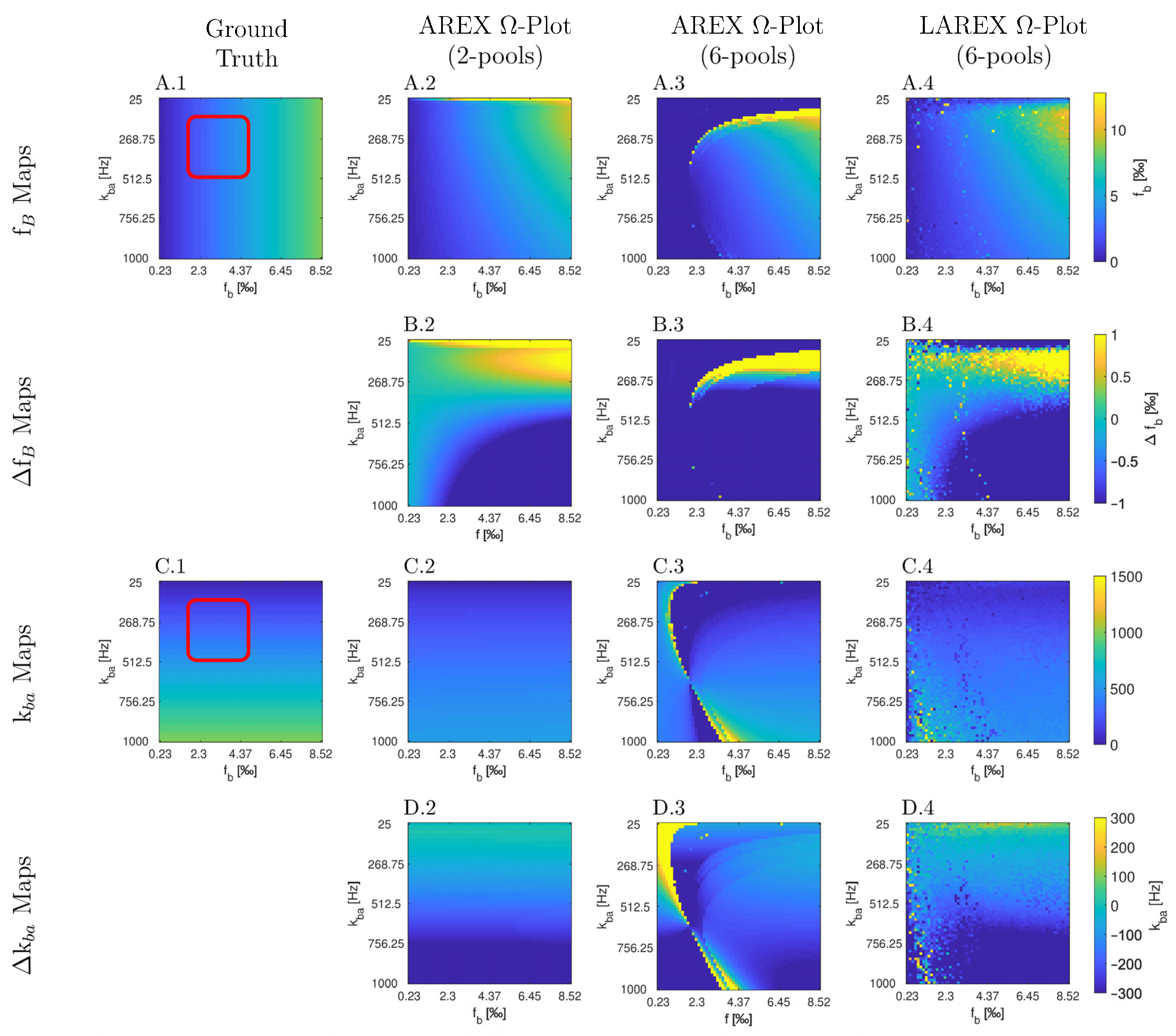
2.1. In Silico Study
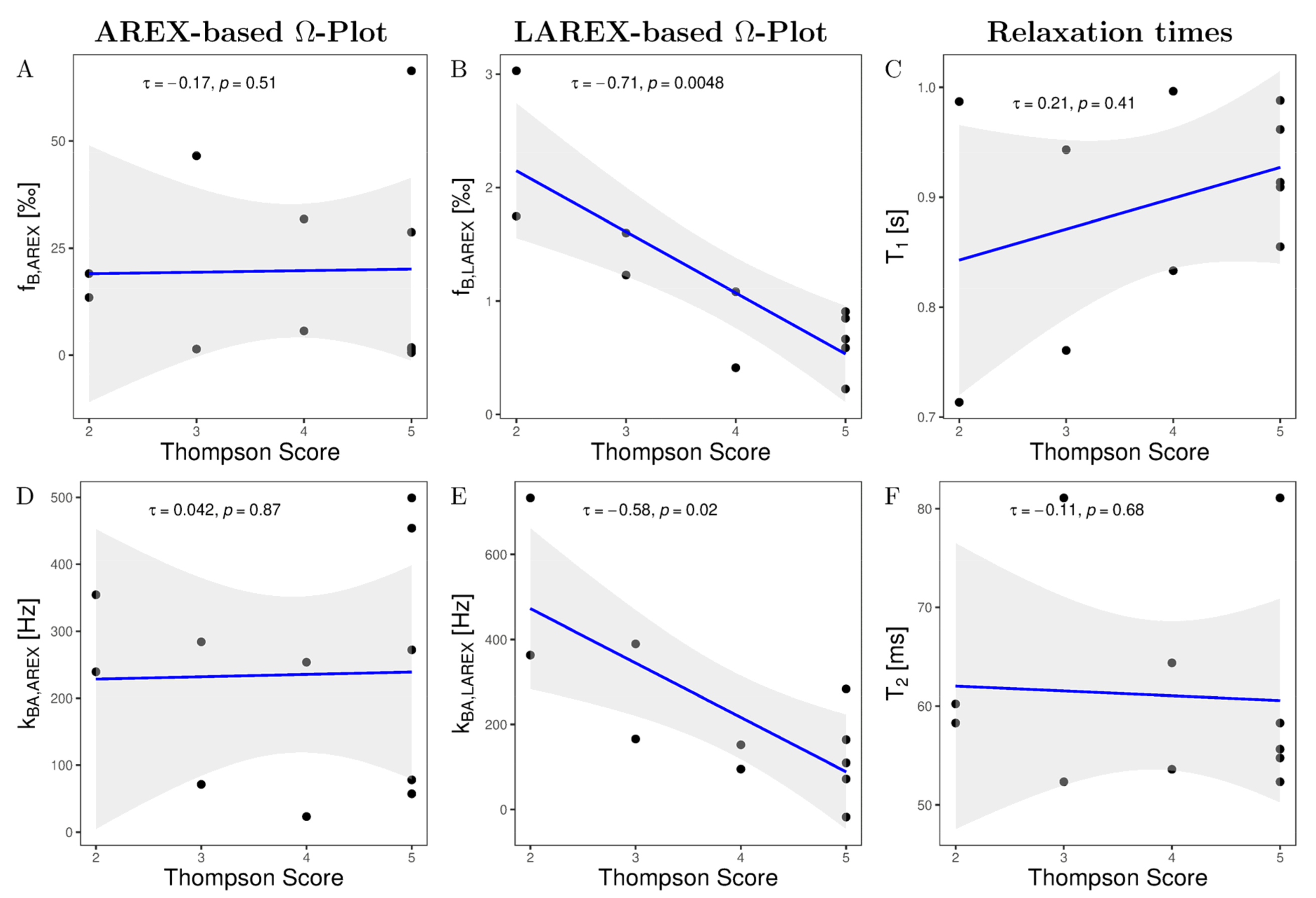
2.2. In Situ Study
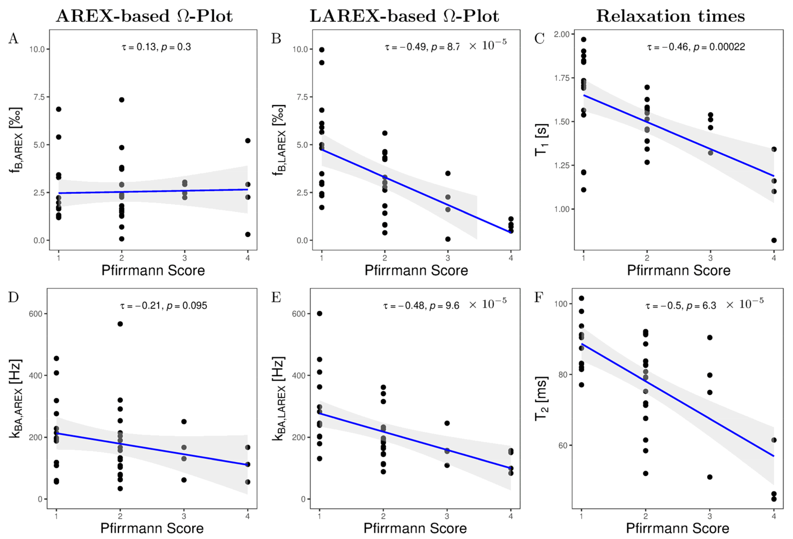
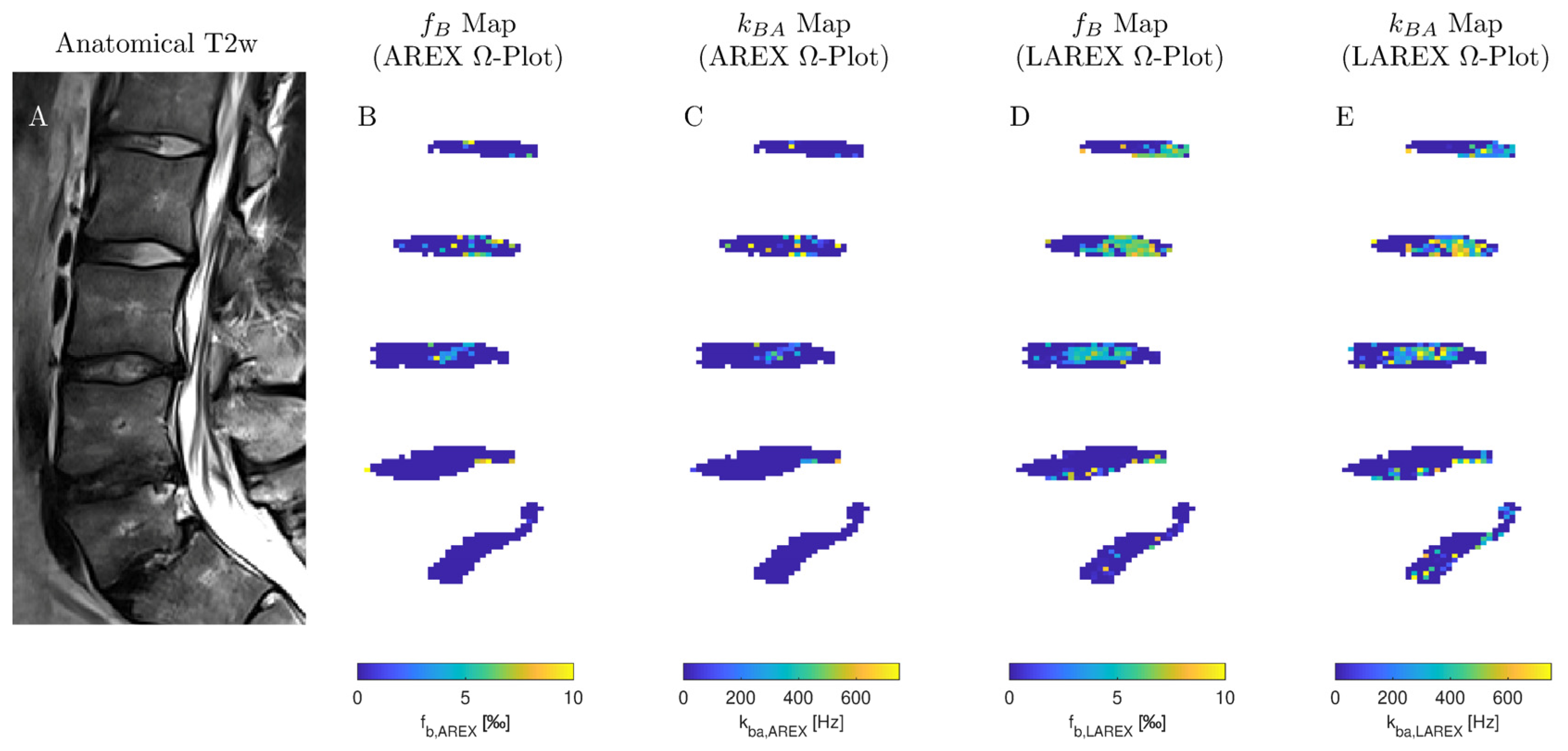
2.3. In Vivo Study
3. Discussion
4. Materials and Methods
4.1. Study Design
4.2. MR Imaging
4.3. In Silico Study
4.4. In Situ Study
4.5. In Vivo Study
4.6. LAREX: Lorentzian-Corrected Apparent Exchange-Dependent Relaxation
4.7. MR Image Analysis
4.8. Statistical Analysis
5. Conclusions
Author Contributions
Funding
Institutional Review Board Statement
Informed Consent Statement
Data Availability Statement
Acknowledgments
Conflicts of Interest
Appendix A


Appendix B


References
- Fatoye, F.; Gebrye, T.; Odeyemi, I. Real-world incidence and prevalence of low back pain using routinely collected data. Rheumatol. Int. 2019, 39, 619–626. [Google Scholar] [CrossRef] [PubMed]
- Suthar, P.; Patel, R.; Mehta, C.; Patel, N. Mri Evaluation of Lumbar Disc Degenerative Disease. J. Clin. Diagn. Res. JCDR 2015, 9, Tc04–Tc09. [Google Scholar] [CrossRef] [PubMed]
- Frenken, M.; Nebelung, S.; Schleich, C.; Müller-Lutz, A.; Radke, K.; Kamp, B.; Boschheidgen, M.; Wollschläger, L.; Bittersohl, B.; Antoch, G.; et al. Non-Specific Low Back Pain and Lumbar Radiculopathy: Comparison of Morphologic and Compositional MRI as Assessed by gagCEST Imaging at 3T. Diagnostics 2021, 11, 402. [Google Scholar] [CrossRef] [PubMed]
- Wollschläger, L.; Nebelung, S.; Schleich, C.; Müller-Lutz, A.; Radke, K.; Frenken, M.; Boschheidgen, M.; Prost, M.; Antoch, G.; Konieczny, M.; et al. Evaluating Lumbar Intervertebral Disc Degeneration on a Compositional Level Using Chemical Exchange Saturation Transfer: Preliminary Results in Patients with Adolescent Idiopathic Scoliosis. Diagnostics 2021, 11, 934. [Google Scholar] [CrossRef] [PubMed]
- Kamp, B.; Frenken, M.; Henke, J.M.; Abrar, D.B.; Nagel, A.M.; Gast, L.V.; Oeltzschner, G.; Wilms, L.M.; Nebelung, S.; Antoch, G.; et al. Quantification of Sodium Relaxation Times and Concentrations As Surrogates of Proteo-glycan Content of Patellar Cartilage at 3t MRI. Diagnostics 2021, 11, 2301. [Google Scholar] [CrossRef] [PubMed]
- Truhn, D.; Zwingenberger, K.T.; Schock, J.; Abrar, D.B.; Radke, K.L.; Post, M.; Linka, K.; Knobe, M.; Kuhl, C.; Nebelung, S. No Pressure, No Diamonds?—Static vs. Dynamic Compressive In-Situ Loading to Evaluate Human Articular Cartilage Functionality by Functional MRI. J. Mech. Behav. Biomed. Mater. 2021, 120, 104558. [Google Scholar] [CrossRef]
- Thiel, T.A.; Schweitzer, J.; Xia, T.; Bechler, E.; Valentin, B.; Steuwe, A.; Boege, F.; Westenfeld, R.; Wittsack, H.-J.; Ljimani, A. Evaluation of Radiographic Contrast-Induced Nephropathy by Functional Diffusion Weighted Imaging. J. Clin. Med. 2021, 10, 4573. [Google Scholar] [CrossRef]
- Müller-Lutz, A.; Ljimani, A.; Stabinska, J.; Zaiss, M.; Boos, J.; Wittsack, H.-J.; Schleich, C. Comparison of B0 versus B0 and B1 field inhomogeneity correction for glycosaminoglycan chemical exchange saturation transfer imaging. Magn. Reson. Mater. Phys. Biol. Med. 2018, 31, 645–651. [Google Scholar] [CrossRef]
- Sasisekharan, R.; Raman, R.; Prabhakar, V. Glycomics Approach to Structure-Function Relationships of Glycosaminoglycans. Annu. Rev. Biomed. Eng. 2006, 8, 181–231. [Google Scholar] [CrossRef]
- Ling, W.; Regatte, R.R.; Navon, G.; Jerschow, A. Assessment of glycosaminoglycan concentration in vivo by chemical exchange-dependent saturation transfer (gagCEST). Proc. Natl. Acad. Sci. USA 2008, 105, 2266–2270. [Google Scholar] [CrossRef]
- Schiebler, T.H. (Ed.) Anatomie: Zytologie, Histologie, Entwicklungsgeschichte, Makroskopische Und Mikroskopische Anatomie Des Menschen; Unter Berücksichtigung Des Gegenstandskatalogs; Mit 119 Tabellen; Springer: Berlin/Heidelberg, Germany, 1999. [Google Scholar]
- Ward, K.M.; Aletras, A.H.; Balaban, R.S. A New Class of Contrast Agents for MRI Based on Proton Chemical Exchange De-pendent Saturation Transfer (Cest). J. Magn. Reson. 2000, 143, 79–87. [Google Scholar] [CrossRef] [PubMed]
- Radke, K.L.; Abrar, D.B.; Frenken, M.; Wilms, L.M.; Kamp, B.; Boschheidgen, M.; Liebig, P.; Ljimani, A.; Filler, T.J.; Antoch, G.; et al. Chemical Exchange Saturation Transfer for Lactate-Weighted Imaging at 3 T MRI: Comprehensive In Silico, In Vitro, In Situ, and In Vivo Evaluations. Tomography 2022, 8, 1277–1292. [Google Scholar] [CrossRef] [PubMed]
- Sun, P.Z. Simplified and scalable numerical solution for describing multi-pool chemical exchange saturation transfer (CEST) MRI contrast. J. Magn. Reson. 2010, 205, 235–241. [Google Scholar] [CrossRef] [PubMed]
- Sun, P.Z.; Wang, Y.; Xiao, G.; Wu, R. Simultaneous experimental determination of labile proton fraction ratio and exchange rate with irradiation radio frequency power-dependent quantitative CEST MRI analysis. Contrast Media Mol. Imaging 2013, 8, 246–251. [Google Scholar] [CrossRef] [PubMed]
- Zhang, S.; Malloy, A.C.R.; Sherry, A.D. MRI Thermometry Based on PARACEST Agents. J. Am. Chem. Soc. 2005, 127, 17572–17573. [Google Scholar] [CrossRef]
- Stabinska, J.; Cronenberg, T.; Wittsack, H.-J.; Lanzman, R.S.; Müller-Lutz, A. Quantitative pulsed CEST-MRI at a clinical 3T MRI system. Magn. Reson. Mater. Phys. Biol. Med. 2017, 30, 505–516. [Google Scholar] [CrossRef]
- Vinogradov, E.; Sherry, D.; Lenkinski, R. CEST: From basic principles to applications, challenges and opportunities. J. Magn. Reson. 2012, 229, 155–172. [Google Scholar] [CrossRef]
- Abrar, D.B.; Schleich, C.; Radke, K.L.; Frenken, M.; Stabinska, J.; Ljimani, A.; Wittsack, H.-J.; Antoch, G.; Bittersohl, B.; Hesper, T.; et al. Detection of early cartilage degeneration in the tibiotalar joint using 3 T gagCEST imaging: A feasibility study. Magn. Reson. Mater. Phys. Biol. Med. 2020, 34, 249–260. [Google Scholar] [CrossRef]
- Dixon, W.T.; Ren, J.; Lubag, A.J.M.; Ratnakar, J.; Vinogradov, E.; Hancu, I.; Lenkinski, R.E.; Sherry, A.D. A Concentration-Independent Method to Measure Exchange Rates in Paracest Agents. Magn. Reson. Med. 2010, 63, 625–632. [Google Scholar] [CrossRef]
- Meissner, J.-E.; Goerke, S.; Rerich, E.; Klika, K.D.; Radbruch, A.; Ladd, M.E.; Bachert, P.; Zaiss, M. Quantitative pulsed CEST-MRI using Ω-plots. NMR Biomed. 2015, 28, 1196–1208. [Google Scholar] [CrossRef]
- Sun, P.Z.; Wang, Y.; Dai, Z.; Xiao, G.; Wu, R. Quantitative chemical exchange saturation transfer (qCEST) MRI-RF spillover effect-corrected omega plot for simultaneous determination of labile proton fraction ratio and exchange rate. Contrast Media Mol. Imaging 2014, 9, 268–275. [Google Scholar] [CrossRef] [PubMed]
- Zaiss, M.; Xu, J.; Goerke, S.; Khan, I.S.; Singer, R.J.; Gore, J.C.; Gochberg, D.F.; Bachert, P. Inverse Z-Spectrum Analysis for Spillover-, Mt-, and T1 -Corrected Steady-State Pulsed Cest-MRI—Application to Ph-Weighted MRI of Acute Stroke. NMR Biomed. 2014, 27, 240–252. [Google Scholar] [CrossRef]
- Warnert, E.A.H.; Wood, T.C.; Incekara, F.; Barker, G.J.; Vincent, A.J.P.; Schouten, J.; Kros, J.M.; Bent, M.V.D.; Smits, M.; Tamames, J.A.H. Mapping tumour heterogeneity with pulsed 3D CEST MRI in non-enhancing glioma at 3 T. Magn. Reson. Mater. Phys. Biol. Med. 2021, 35, 53–62. [Google Scholar] [CrossRef] [PubMed]
- Zhang, X.-Y.; Wang, F.; Li, H.; Xu, J.; Gochberg, D.F.; Gore, J.C.; Zu, Z. Accuracy in the quantification of chemical exchange saturation transfer (CEST) and relayed nuclear Overhauser enhancement (rNOE) saturation transfer effects. NMR Biomed. 2017, 30, e3716. [Google Scholar] [CrossRef] [PubMed]
- Schüre, J.; Shrestha, M.; Breuer, S.; Deichmann, R.; Hattingen, E.; Wagner, M.; Pilatus, U. The pH sensitivity of APT-CEST using phosphorus spectroscopy as a reference method. NMR Biomed. 2019, 32, e4125. [Google Scholar] [CrossRef]
- Zaiß, M.; Schmitt, B.; Bachert, P. Quantitative separation of CEST effect from magnetization transfer and spillover effects by Lorentzian-line-fit analysis of z-spectra. J. Magn. Reson. 2011, 211, 149–155. [Google Scholar] [CrossRef]
- Singh, A.; Haris, M.; Cai, K.; Kassey, V.B.; Kogan, F.; Reddy, D.; Hariharan, H.; Reddy, R. Chemical exchange saturation transfer magnetic resonance imaging of human knee cartilage at 3 T and 7 T. Magn. Reson. Med. 2011, 68, 588–594. [Google Scholar] [CrossRef]
- Thompson, J.P.; Pearce, R.H.; Schechter, M.T.; Adams, M.E.; Tsang, I.K.Y.; Bishop, P.B. Preliminary Evaluation of a Scheme for Grading the Gross Morphology of the Human Intervertebral Disc. Spine 1990, 15, 411–415. [Google Scholar] [CrossRef]
- Pfirrmann, C.; Metzdorf, A.; Zanetti, M.; Hodler, J.; Boos, N. Magnetic Resonance Classification of Lumbar Intervertebral Disc Degeneration. Spine 2001, 26, 1873–1878. [Google Scholar] [CrossRef]
- Zhou, Z.; Bez, M.; Tawackoli, W.; Giaconi, J.; Sheyn, D.; De Mel, S.; Maya, M.M.; Pressman, B.D.; Gazit, Z.; Pelled, G.; et al. Quantitative chemical exchange saturation transfer MRI of intervertebral disc in a porcine model. Magn. Reson. Med. 2016, 76, 1677–1683. [Google Scholar] [CrossRef]
- Müller-Lutz, A.; Schleich, C.; Pentang, G.; Schmitt, B.; Lanzman, R.S.; Matuschke, F.; Wittsack, H.-J.; Miese, F. Age-dependency of glycosaminoglycan content in lumbar discs: A 3t gagcEST study. J. Magn. Reson. Imaging 2015, 42, 1517–1523. [Google Scholar] [CrossRef] [PubMed]
- Kauppinen, J.K.; Moffatt, D.J.; Mantsch, H.H.; Cameron, D.G. Smoothing of spectral data in the Fourier domain. Appl. Opt. 1982, 21, 1866–1872. [Google Scholar] [CrossRef] [PubMed]
- Iatridis, J.C.; MacLean, J.J.; O’Brien, M.; Stokes, I. Measurements of Proteoglycan and Water Content Distribution in Human Lumbar Intervertebral Discs. Spine 2007, 32, 1493–1497. [Google Scholar] [CrossRef] [PubMed]
- Roughley, F.J. The structure and function of cartilage proteoglycans. Eur. Cells Mater. 2006, 12, 92–101. [Google Scholar] [CrossRef]
- Radke, K.; Wollschläger, L.; Nebelung, S.; Abrar, D.; Schleich, C.; Boschheidgen, M.; Frenken, M.; Schock, J.; Klee, D.; Frahm, J.; et al. Deep Learning-Based Post-Processing of Real-Time MRI to Assess and Quantify Dynamic Wrist Movement in Health and Disease. Diagnostics 2021, 11, 1077. [Google Scholar] [CrossRef]
- Schock, J.; Truhn, D.; Nürnberger, D.; Conrad, S.; Huppertz, M.S.; Keil, S.; Kuhl, C.; Merhof, D.; Nebelung, S. Artificial Intel-ligence-Based Automatic Assessment of Lower Limb Torsion on MRI. Sci. Rep. 2021, 11, 23244. [Google Scholar] [CrossRef]
- Müller-Franzes, G.; Nolte, T.; Ciba, M.; Schock, J.; Khader, F.; Prescher, A.; Wilms, L.M.; Kuhl, C.; Nebelung, S.; Truhn, D. Fast, Accurate, and Robust T2 Mapping of Articular Cartilage by Neural Networks. Diagnostics 2022, 12, 688. [Google Scholar] [CrossRef]
- Zaiss, M.; Deshmane, A.; Schuppert, M.; Herz, K.; Glang, F.; Ehses, P.; Lindig, T.; Bender, B.; Ernemann, U.; Scheffler, K. DeepCEST: 9.4 T Chemical exchange saturation transfer MRI contrast predicted from 3 T data—A proof of concept study. Magn. Reson. Med. 2019, 81, 3901–3914. [Google Scholar] [CrossRef]
- Huang, J.; Lai, J.H.C.; Tse, K.; Cheng, G.W.Y.; Liu, Y.; Chen, Z.; Han, X.; Chen, L.; Xu, J.; Chan, K.W.Y. Deep neural network based CEST and AREX processing: Application in imaging a model of Alzheimer’s disease at 3 T. Magn. Reson. Med. 2021, 87, 1529–1545. [Google Scholar] [CrossRef]
- Wei, W.; Jia, G.; Flanigan, D.; Zhou, J.; Knopp, M.V. Chemical exchange saturation transfer MR imaging of articular cartilage glycosaminoglycans at 3T: Accuracy of B0 Field Inhomogeneity corrections with gradient echo method. Magn. Reson. Imaging 2013, 32, 41–47. [Google Scholar] [CrossRef]
- Liu, D.; Zhou, J.; Xue, R.; Wang, D.J.J. Using simultaneous multi-slice excitation to accelerate CEST imaging. In Proceedings of the 22nd Annual Meeting of ISMRM, Milan, Italy, 10–16 May 2014; p. 3294. [Google Scholar]
- Randtke, E.A.; Granados, J.; Howison, C.M.; Pagel, M.D.; Cárdenas-Rodríguez, J. Multislice CEST MRI improves the spatial assessment of tumor pH. Magn. Reson. Med. 2016, 78, 97–106. [Google Scholar] [CrossRef] [PubMed]
- Boutin, C.; Léonce, E.; Brotin, T.; Jerschow, A.; Berthault, P. Ultrafast Z-Spectroscopy for 129Xe NMR-Based Sensors. J. Phys. Chem. Lett. 2013, 4, 4172–4176. [Google Scholar] [CrossRef] [PubMed][Green Version]
- Heo, H.; Zhang, Y.; Lee, D.-H.; Jiang, S.; Zhao, X.; Zhou, J. Accelerating chemical exchange saturation transfer (CEST) MRI by combining compressed sensing and sensitivity encoding techniques. Magn. Reson. Med. 2016, 77, 779–786. [Google Scholar] [CrossRef] [PubMed]
- Zhang, Y.; Zu, T.; Liu, R.; Zhou, J. Acquisition sequences and reconstruction methods for fast chemical exchange saturation transfer imaging. NMR Biomed. 2022, e4699. [Google Scholar] [CrossRef]
- Zaiss, M.; Bachert, P. Chemical Exchange Saturation Transfer (Cest) and Mr Z-Spectroscopy In Vivo: A Review of Theoretical Approaches and Methods. Phys. Med. Biol. 2013, 58, R221–R269. [Google Scholar] [CrossRef]
- Buades, A.; Coll, B.; Morel, J.-M. A non-local algorithm for image denoising. In Proceedings of the 2005 IEEE Computer Society Conference on Computer Vision and Pattern Recognition (Cvpr’05)—Workshops, San Diego, CA, USA, 20–25 June 2005; pp. 60–65. [Google Scholar]
- Kubaski, F.; Osago, H.; Mason, R.W.; Yamaguchi, S.; Kobayashi, H.; Tsuchiya, M.; Orii, T.; Tomatsu, S. Glycosaminoglycans detection methods: Applications of mass spectrometry. Mol. Genet. Metab. 2016, 120, 67–77. [Google Scholar] [CrossRef]
- Stover, J.D.; Lawrence, B.; Bowles, R.D. Degenerative IVD conditioned media and acidic pH sensitize sensory neurons to cyclic tensile strain. J. Orthop. Res. 2020, 39, 1192–1203. [Google Scholar] [CrossRef]
- Kim, M.; Gillen, J.; Landman, B.A.; Zhou, J.; Van Zijl, P.C.M. Water Saturation Shift Referencing (Wassr) for Chemical Exchange Saturation Transfer (Cest) Experiments. Magn. Reson. Med. 2009, 61, 1441–1450. [Google Scholar] [CrossRef]
- Schuenke, P.; Windschuh, J.; Roeloffs, V.; Ladd, M.E.; Bachert, P.; Zaiss, M. Simultaneous Mapping of Water Shift and B1 (Wasabi)-Application To Field-Inhomogeneity Correction of Cest MRI Data. Magn. Reson. Med. 2017, 77, 571–580. [Google Scholar] [CrossRef]
- Schmitt, B.; Zaiß, M.; Zhou, J.; Bachert, P. Optimization of pulse train presaturation for CEST imaging in clinical scanners. Magn. Reson. Med. 2011, 65, 1620–1629. [Google Scholar] [CrossRef]
- Roeloffs, V.; Meyer, C.; Bachert, P.; Zaiss, M. Towards quantification of pulsed spinlock and CEST at clinical MR scanners: An analytical interleaved saturation-relaxation (ISAR) approach. NMR Biomed. 2014, 28, 40–53. [Google Scholar] [CrossRef] [PubMed]
- Zaiss, M.; Angelovski, G.; Demetriou, E.; McMahon, M.T.; Golay, X.; Scheffler, K. QUESP and QUEST revisited—Fast and accurate quantitative CEST experiments. Magn. Reson. Med. 2017, 79, 1708–1721. [Google Scholar] [CrossRef] [PubMed]
- Wada, T.; Togao, O.; Tokunaga, C.; Funatsu, R.; Yamashita, Y.; Kobayashi, K.; Nakamura, Y.; Honda, H. Glycosaminoglycan chemical exchange saturation transfer in human lumbar intervertebral discs: Effect of saturation pulse and relationship with low back pain. J. Magn. Reson. Imaging 2016, 45, 863–871. [Google Scholar] [CrossRef] [PubMed]
- Agarwal, V.; Linser, R.; Fink, U.; Faelber, K.; Reif, B. Identification of Hydroxyl Protons, Determination of Their Exchange Dynamics, and Characterization of Hydrogen Bonding in a Microcrystallin Protein. J. Am. Chem. Soc. 2010, 132, 3187–3195. [Google Scholar] [CrossRef] [PubMed]
- Wilms, L.M.; Radke, K.L.; Abrar, D.B.; Latz, D.; Schock, J.; Frenken, M.; Windolf, J.; Antoch, G.; Filler, T.J.; Nebelung, S. Micro- and Macroscale Assessment of Posterior Cruciate Ligament Functionality Based on Advanced MRI Techniques. Diagnostics 2021, 11, 1790. [Google Scholar] [CrossRef]
- Ishikawa, T.; Watanabe, A.; Kamoda, H.; Miyagi, M.; Inoue, G.; Takahashi, K.; Ohtori, S. Evaluation of Lumbar Intervertebral Disc Degeneration Using T1ρ and T2 Magnetic Resonance Imaging in a Rabbit Disc Injury Model. Asian Spine J. 2018, 12, 317–324. [Google Scholar] [CrossRef]
- Waltz, R.; Morales, J.; Nocedal, J.; Orban, D. An interior algorithm for nonlinear optimization that combines line search and trust region steps. Math. Program. 2006, 107, 391–408. [Google Scholar] [CrossRef]
- Masnadi-Shirazi, H.; Mahadevan, V.; Vasconcelos, N. On the design of robust classifiers for computer vision. In Proceedings of the 2010 IEEE Computer Society Conference on Computer Vision and Pattern Recognition, San Francisco, CA, USA, 13–18 June 2010; pp. 779–786. [Google Scholar]
- Yushkevich, P.A.; Piven, J.; Hazlett, H.C.; Smith, R.G.; Ho, S.; Gee, J.C.; Gerig, G. User-guided 3D active contour segmentation of anatomical structures: Significantly improved efficiency and reliability. NeuroImage 2006, 31, 1116–1128. [Google Scholar] [CrossRef]
- Cohen, J. Statistical Power Analysis for the Behavioral Sciences; Routledge: London, UK, 2013. [Google Scholar]
- Koo, T.K.; Li, M.Y. A Guideline of Selecting and Reporting Intraclass Correlation Coefficients for Reliability Research. J. Chiropr. Med. 2016, 15, 155–163. [Google Scholar] [CrossRef]
- Shrout, P.E.; Fleiss, J.L. Intraclass Correlations: Uses in Assessing Rater Reliability. Psychol. Bull. 1979, 86, 420–428. [Google Scholar] [CrossRef]
- Armstrong, R.A. When to Use the Bonferroni Correction. Ophthalmic Physiol. Opt. 2014, 34, 502–508. [Google Scholar] [CrossRef] [PubMed]
- Mougin, O.; Clemence, M.; Peters, A.; Pitiot, A.; Gowland, P. High-resolution imaging of magnetisation transfer and nuclear Overhauser effect in the human visual cortex at 7 T. NMR Biomed. 2013, 26, 1508–1517. [Google Scholar] [CrossRef] [PubMed]
- Shah, S.M.; Mougin, O.E.; Carradus, A.J.; Geades, N.; Dury, R.; Morley, W.; Gowland, P.A. The z-spectrum from human blood at 7T. NeuroImage 2017, 167, 31–40. [Google Scholar] [CrossRef] [PubMed]
- Singh, A.; Debnath, A.; Cai, K.; Bagga, P.; Haris, M.; Hariharan, H.; Reddy, R. Evaluating the feasibility of creatine-weighted CEST MRI in human brain at 7 T using a Z-spectral fitting approach. NMR Biomed. 2019, 32, e4176. [Google Scholar] [CrossRef] [PubMed]


| Water [8] | Hydroxyl [28] | Amide [25] | NOE #1 [25] | NOE #2 [25] | MT [25] | |
|---|---|---|---|---|---|---|
| Pool | A | B | C | D | E | F |
| T1 (ms) | 1306 | T1,a | T1,a | T1,a | T1,a | T1,a |
| T2 (ms) | 134 | 10 | 2 | 1 | 0.5 | 0.015 |
| f | 1 | variable | 1/3 × fB | 0.003 | 0.007 | 0.1 |
| kba (Hz) | - | variable | 50 | 50 | 50 | 25 |
| Δ (ppm) | 0 | 1 | 3.5 | −1.6 | −3.5 | −2.3 |
| Parameter | Pfirrmann Score | AREX-Based Ω-Analyses | LAREX-Based Ω-Analyses |
|---|---|---|---|
| fb [‰] | 1 | 2.49 ± 1.71 | 4.96 ± 2.54 |
| 2 | 2.48 ± 1.68 | 3.04 ± 1.52 | |
| 3 | 2.48 ± 1.67 | 1.85 ± 1.43 | |
| 4 | 2.67 ± 0.38 | 0.79 ± 0.26 | |
| kba [Hz] | 1 | 215.7 ± 118.2 | 292.2 ± 125.5 |
| 2 | 175.2 ± 127.1 | 199.5 ± 76.0 | |
| 3 | 152.6 ± 78.7 | 166.7 ± 57.1 | |
| 4 | 80.9 ± 76.5 | 122.6 ± 36.4 |
| T1w TSE | T2w TSE * | T1 Mapping A | T2-SE Mapping | CEST In Situ C | CEST In Vivo D | WASSR | |
|---|---|---|---|---|---|---|---|
| Orientation | sag | sag | sag | sag | sag | sag | sag |
| TE (ms) | 9.8 | 95 | 10 | B | 3.5 | 3.5 | 3.5 |
| TR (ms) | 650 | 3500 | 6000 | 1000 | 2500 | 2500 | 2500 |
| Slices | 15 | 15 | 1 | 1 | 1 | 1 | 1 |
| Slice Thickness (mm) | 3 | 4 | 4 | 4 | 4 | 6 | 4/6 |
| FOV (mm × mm) | 300 × 300 | 260 × 260 | 200 × 200 | 200 × 200 | 200 × 200 | 200 × 200 | 200 × 200 |
| Image matrix (pixel) | 384 × 384 | 384 × 384 | 128 × 128 | 128 × 128 | 128 × 128 | 128 × 128 | 128 × 128 |
| Flip angle (°) | 150 | 160 | 180 | 180 | 15 | 15 | 15 |
| Turbo Factor | 109 | 17 | 11 | na | na | na | na |
| GRAPPA | 2 | na | 2 | na | na | na | na |
| Duration (min:s) | 1:12 | 3:46 | 8:38 | 1:12 | 84:35 | 36:15 | 3:43 |
| *—only in vivo A—TI = 25, 50, 100, 500, 1000, 2000 and 3000 ms B—TE = 9.7 ms to 197 ms with a step size of 9.7 ms C—B1 = 0.6, 0.7, 0.8, 0.9, 1.0, 1.1, 1.2 µT; tp = 100; td = 100 ms and np = 40 D—B1 = 0.6, 0.9, 1.2 µT; tp = 100 ms; td = 100 ms and np = 40 | |||||||
| Awater | Wwater | Δwater | Aamide | Wamide | Δamide | Ahydroxyl | Whydroxyl | Δhydroxyl | |
|---|---|---|---|---|---|---|---|---|---|
| Start | 0.85 | 2 | 0 | 0.01 | 1 | 3.5 | 0.01 | 1 | 1 |
| Lower | 0.5 | 1 | −0.5 | 0 | 0.2 | 3 | 0 | 0.5 | 0.6 |
| Upper | 1.1 | 6 | 0.5 | 0.1 | 3 | 4 | 0.1 | 2 | 1.4 |
| ANOE #1 | WNOE #1 | ΔNOE #1 | ANOE #2 | WNOE #2 | ΔNOE #2 | AMT | WMT | ΔMT | |
| Start | 0.001 | 1 | −1.6 | 0.03 | 1 | −3.5 | 0.1 | 10 | −2.3 |
| Lower | 0 | 0.5 | −2.5 | 0 | 0.5 | −5 | 0 | 8 | −3 |
| Upper | 0.1 | 3.5 | −0.5 | 0.2 | 4 | −3 | 0.5 | 20 | −2 |
Publisher’s Note: MDPI stays neutral with regard to jurisdictional claims in published maps and institutional affiliations. |
© 2022 by the authors. Licensee MDPI, Basel, Switzerland. This article is an open access article distributed under the terms and conditions of the Creative Commons Attribution (CC BY) license (https://creativecommons.org/licenses/by/4.0/).
Share and Cite
Radke, K.L.; Wilms, L.M.; Frenken, M.; Stabinska, J.; Knet, M.; Kamp, B.; Thiel, T.A.; Filler, T.J.; Nebelung, S.; Antoch, G.; et al. Lorentzian-Corrected Apparent Exchange-Dependent Relaxation (LAREX) Ω-Plot Analysis—An Adaptation for qCEST in a Multi-Pool System: Comprehensive In Silico, In Situ, and In Vivo Studies. Int. J. Mol. Sci. 2022, 23, 6920. https://doi.org/10.3390/ijms23136920
Radke KL, Wilms LM, Frenken M, Stabinska J, Knet M, Kamp B, Thiel TA, Filler TJ, Nebelung S, Antoch G, et al. Lorentzian-Corrected Apparent Exchange-Dependent Relaxation (LAREX) Ω-Plot Analysis—An Adaptation for qCEST in a Multi-Pool System: Comprehensive In Silico, In Situ, and In Vivo Studies. International Journal of Molecular Sciences. 2022; 23(13):6920. https://doi.org/10.3390/ijms23136920
Chicago/Turabian StyleRadke, Karl Ludger, Lena Marie Wilms, Miriam Frenken, Julia Stabinska, Marek Knet, Benedikt Kamp, Thomas Andreas Thiel, Timm Joachim Filler, Sven Nebelung, Gerald Antoch, and et al. 2022. "Lorentzian-Corrected Apparent Exchange-Dependent Relaxation (LAREX) Ω-Plot Analysis—An Adaptation for qCEST in a Multi-Pool System: Comprehensive In Silico, In Situ, and In Vivo Studies" International Journal of Molecular Sciences 23, no. 13: 6920. https://doi.org/10.3390/ijms23136920
APA StyleRadke, K. L., Wilms, L. M., Frenken, M., Stabinska, J., Knet, M., Kamp, B., Thiel, T. A., Filler, T. J., Nebelung, S., Antoch, G., Abrar, D. B., Wittsack, H.-J., & Müller-Lutz, A. (2022). Lorentzian-Corrected Apparent Exchange-Dependent Relaxation (LAREX) Ω-Plot Analysis—An Adaptation for qCEST in a Multi-Pool System: Comprehensive In Silico, In Situ, and In Vivo Studies. International Journal of Molecular Sciences, 23(13), 6920. https://doi.org/10.3390/ijms23136920