Author Contributions
Conceptualisation, L.Č., A.M., L.Š. and L.D.; Formal analysis, D.G., L.Č. and L.Š.; Methodology, A.M., L.D. and L.Š.; Project administration, L.Č., L.Š. and A.M.; Visualization, A.M., L.Č., and D.G.; Writing of original draft, A.M., L.Č., L.D., D.G. and L.Š.; Writing—review and editing, A.M., L.Č., D.G. and L.D. All authors have read and agreed to the published version of the manuscript.
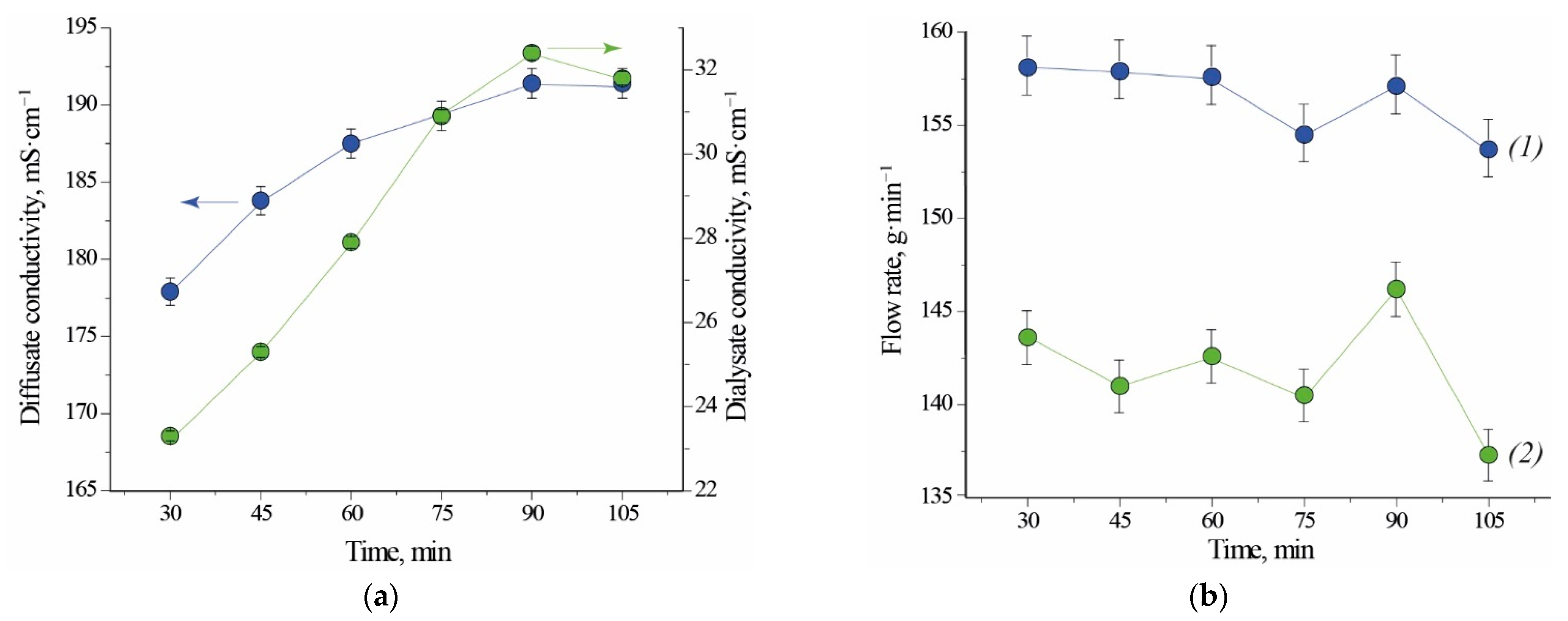
Figure 1.
Conductivity (a) and flow rate (b) as a function of time for Test 1.1. (1) diffusate; (2) dialysate. Initial fill: water. Note that the lines connecting experimental points are not true trendlines.
Figure 1.
Conductivity (a) and flow rate (b) as a function of time for Test 1.1. (1) diffusate; (2) dialysate. Initial fill: water. Note that the lines connecting experimental points are not true trendlines.
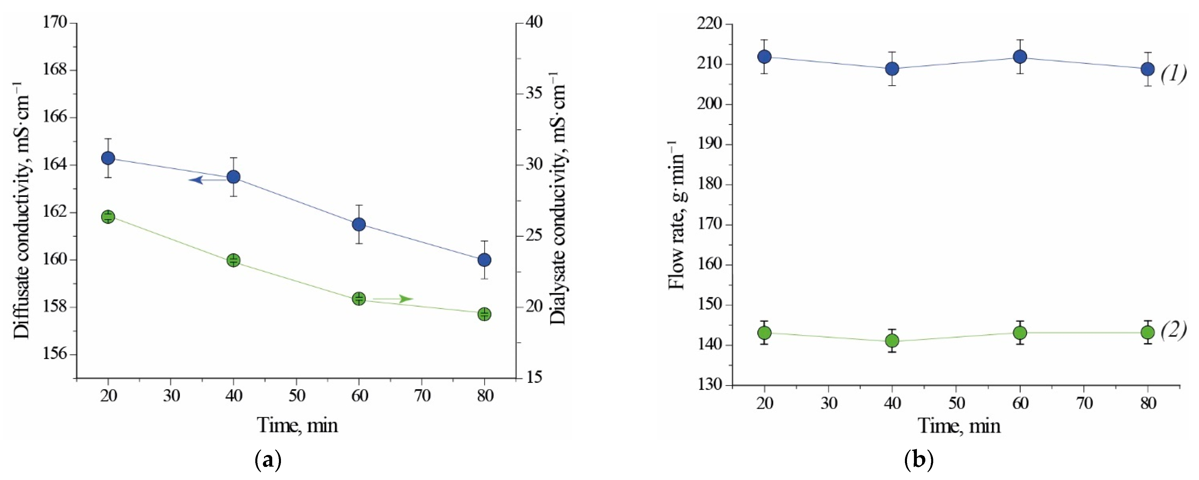
Figure 2.
Conductivity (a) and flow rate (b) as a function of time for Test 2.1. (1) diffusate; (2) dialysate. Initial fill: DD profile from the previous testing. Note that the lines connecting experimental points are not true trendlines.
Figure 2.
Conductivity (a) and flow rate (b) as a function of time for Test 2.1. (1) diffusate; (2) dialysate. Initial fill: DD profile from the previous testing. Note that the lines connecting experimental points are not true trendlines.
Figure 3.
(a) Fourier transform infrared spectroscopy (FT-IR) spectra and (b) stress-strain curves for membranes (1) before use (initial state) and (2) after use (in a dry state, Cl− form).
Figure 3.
(a) Fourier transform infrared spectroscopy (FT-IR) spectra and (b) stress-strain curves for membranes (1) before use (initial state) and (2) after use (in a dry state, Cl− form).
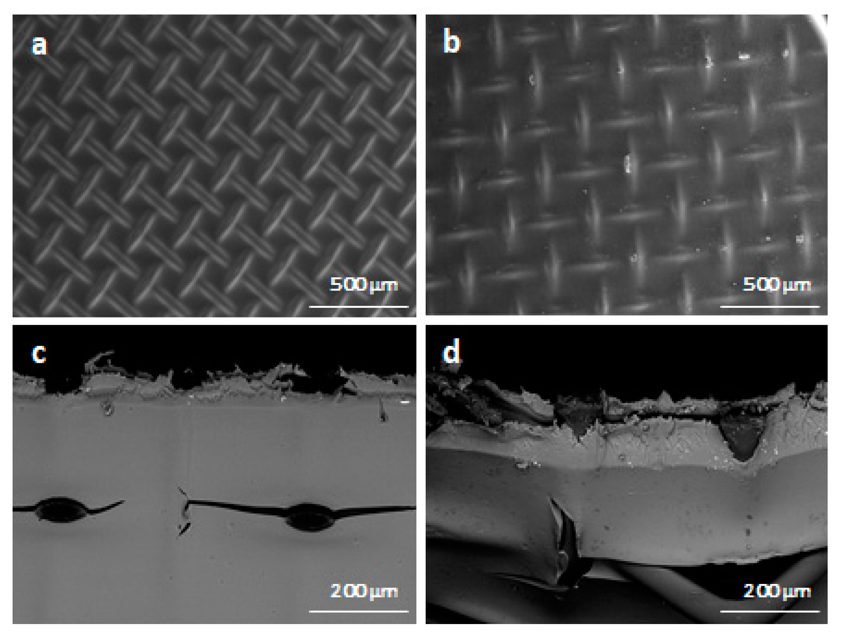
Figure 4.
Scanning electron microscopy images detailing membrane state before use ((a) surface, (c) cross-section)) and after use ((b) surface, (d) cross-section).
Figure 4.
Scanning electron microscopy images detailing membrane state before use ((a) surface, (c) cross-section)) and after use ((b) surface, (d) cross-section).
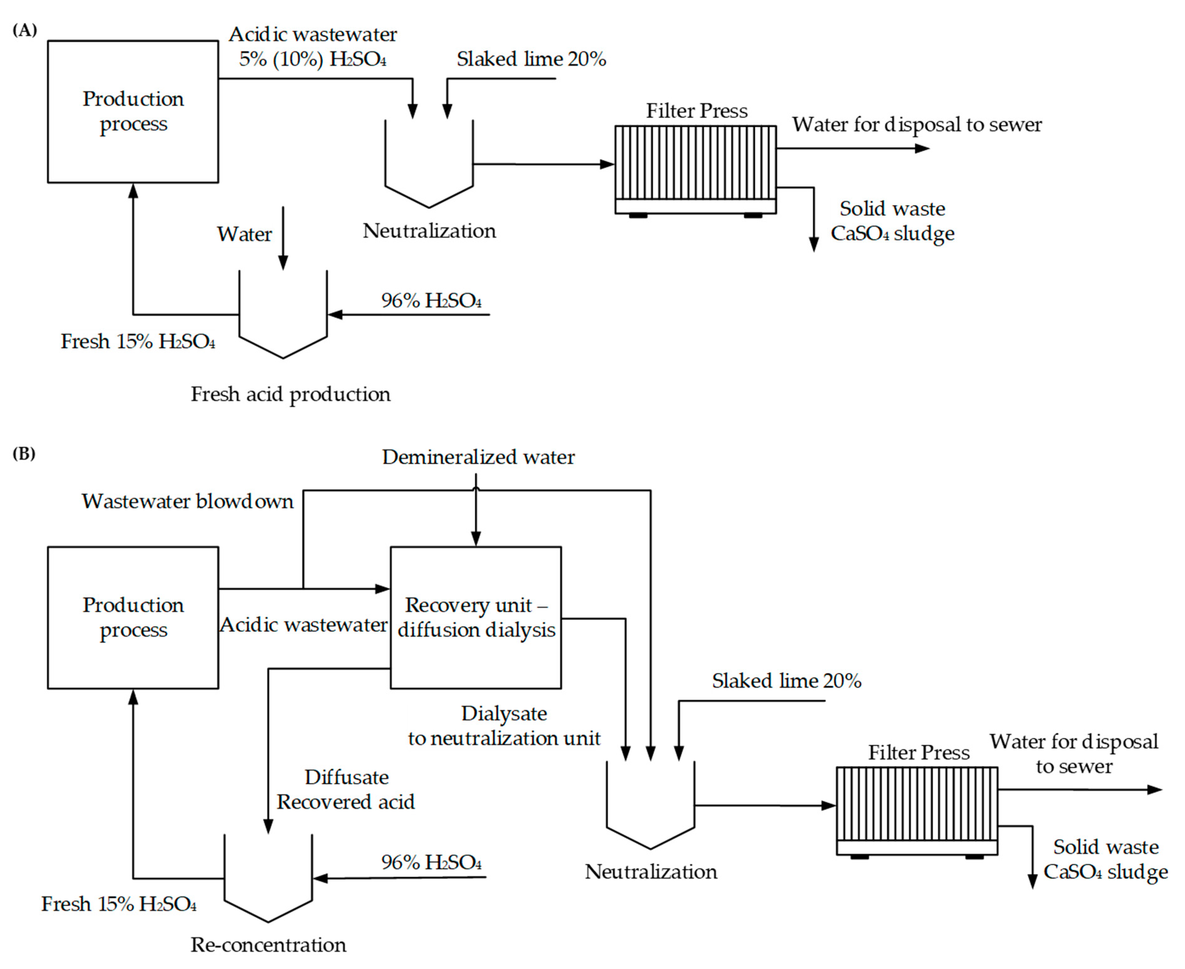
Figure 5.
Process flow diagram for the proposed treatment technology. (A) treatment of acidic wastewater without diffusion dialysis; (B) implementation of dialysis into production-level wastewater management.
Figure 5.
Process flow diagram for the proposed treatment technology. (A) treatment of acidic wastewater without diffusion dialysis; (B) implementation of dialysis into production-level wastewater management.
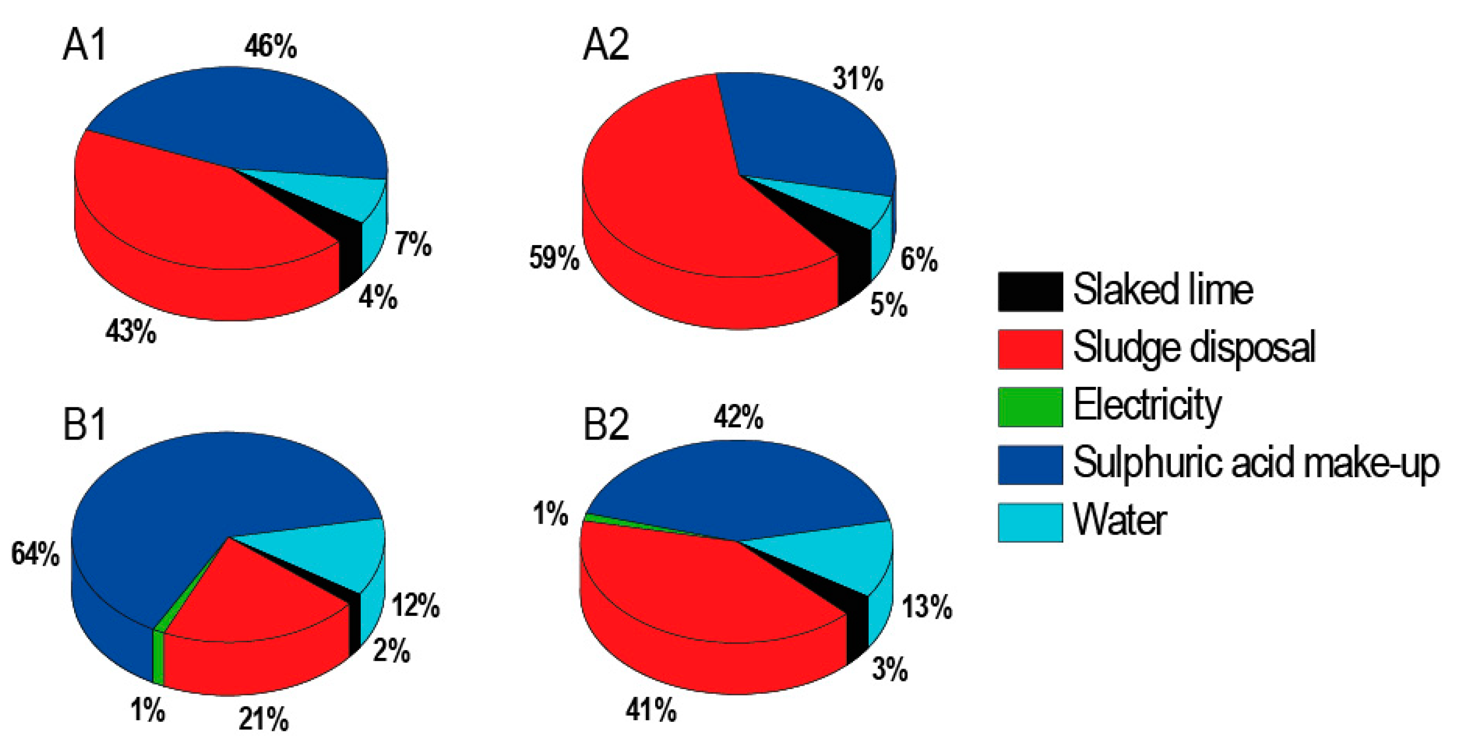
Figure 6.
Percentage distribution of operating expenses: (A1) processing 5% H2SO4 wastewater without DD; (B1) processing 5% H2SO4 wastewater with DD; (A2) processing 10% H2SO4 wastewater without DD; (B2) processing 10% H2SO4 wastewater with DD.
Figure 6.
Percentage distribution of operating expenses: (A1) processing 5% H2SO4 wastewater without DD; (B1) processing 5% H2SO4 wastewater with DD; (A2) processing 10% H2SO4 wastewater without DD; (B2) processing 10% H2SO4 wastewater with DD.
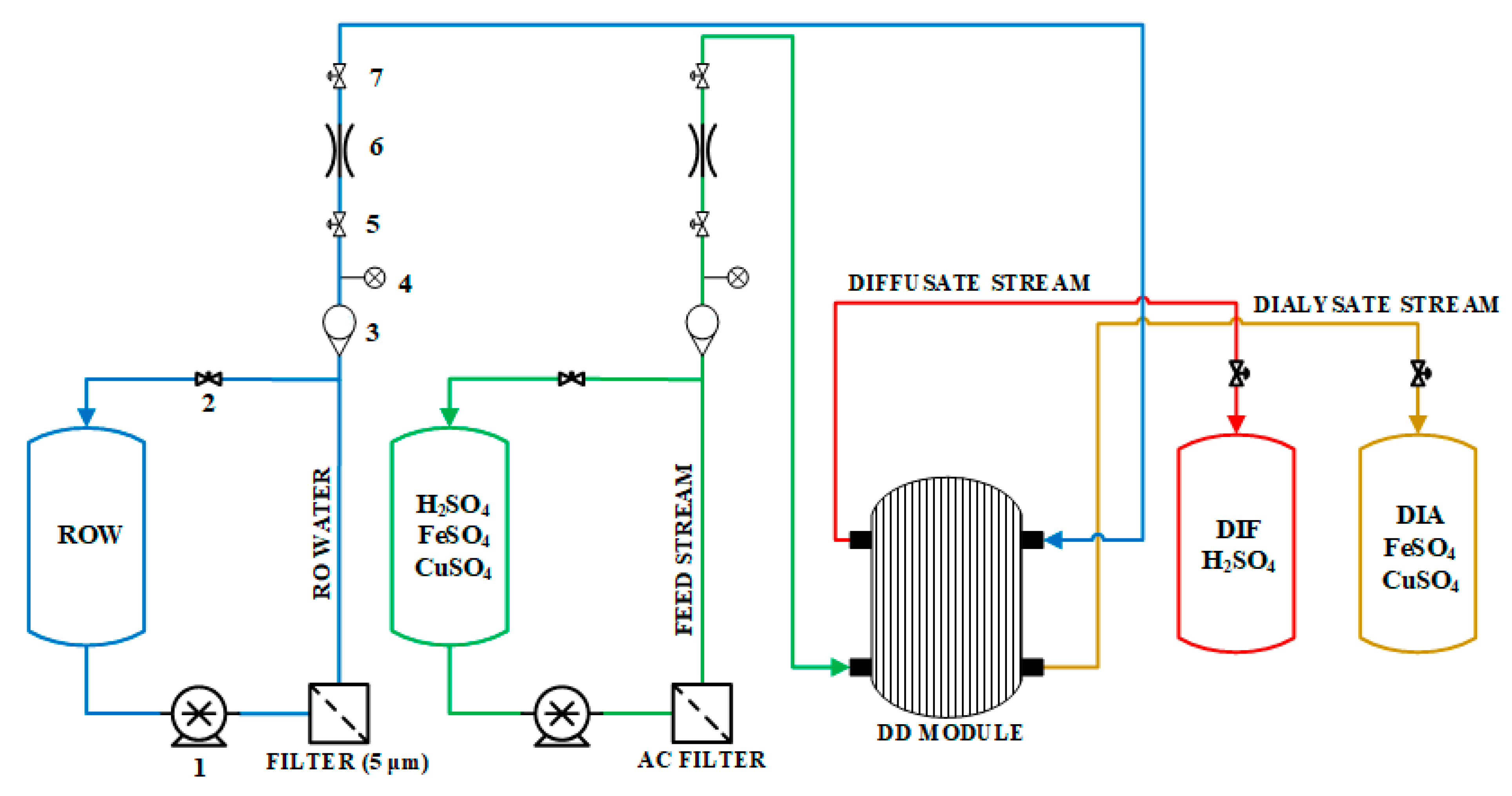
Figure 7.
Simplified process flow diagram of the acid-recovery system. Instrumentation key: (1) pump; (2) needle valve; (3) rotameter; (4) pressure sensor; (5) manual valve; (6) flow control valve; (7) manual valve.
Figure 7.
Simplified process flow diagram of the acid-recovery system. Instrumentation key: (1) pump; (2) needle valve; (3) rotameter; (4) pressure sensor; (5) manual valve; (6) flow control valve; (7) manual valve.
Table 1.
Summarized values for performance parameters used for Tests 1.1 and 2.1. Symbols: Y—yield of acid, RCu2+—rejection of Cu2+, RFe2+—rejection of Fe2+, —flux of acid, —weight fraction of acid in feed (diffusate/dialysate) solution, PFEED (DIF)—ionic purity of feed (diffusate).
Table 1.
Summarized values for performance parameters used for Tests 1.1 and 2.1. Symbols: Y—yield of acid, RCu2+—rejection of Cu2+, RFe2+—rejection of Fe2+, —flux of acid, —weight fraction of acid in feed (diffusate/dialysate) solution, PFEED (DIF)—ionic purity of feed (diffusate).
| Parameter | Unit | Test 1.1 | Test 2.1 |
|---|
| Y | % | 88 ± 5 | 93 ± 6 |
| RCu2+ | % | 95 ± 5 | 90 ± 10 |
| RFe2+ | % | 91 ± 9 | 86 ± 10 |
| g·m−2·h−1 | 81 ± 3 | 87 ± 3 |
| % | 5.18 ± 0.10 | 4.84 ± 0.10 |
| % | 4.39 ± 0.09 | 3.48 ± 0.07 |
| % | 0.66 ± 0.01 | 0.41 ± 0.01 |
| PFEED | % | 76.8 ± 1.3 | 76.0 ± 1.3 |
| PDIF | % | 97.5 ± 0.2 | 95.6 ± 0.3 |
| - | 3.2 | 4.4 |
Table 2.
Flows of inlet and outlet streams (volumetric flows in L·h−1 and mass flows in kg·h−1). Symbols: —volumetric flow rate of feed (RO permeate/diffusate/dialysate), —mass flow rate of feed (RO permeate/diffusate/dialysate).
Table 2.
Flows of inlet and outlet streams (volumetric flows in L·h−1 and mass flows in kg·h−1). Symbols: —volumetric flow rate of feed (RO permeate/diffusate/dialysate), —mass flow rate of feed (RO permeate/diffusate/dialysate).
| Parameter | Test 1.1 | Test 2.1 |
|---|
| 8.55 ± 0.05 | 9.42 ± 0.05 |
| 8.64 ± 0.05 | 11.45 ± 0.05 |
| 8.98 ± 0.09 | 12.28 ± 0.12 |
| 8.21 ± 0.08 | 8.58 ± 0.09 |
| 8.83 ± 0.05 | 9.70 ± 0.05 |
| 8.63 ± 0.05 | 11.42 ± 0.05 |
| 9.22 ± 0.18 | 12.53 ± 0.25 |
| 8.24 ± 0.16 | 8.59 ± 0.17 |
Table 3.
Analytical measurements for Tests 1.1 and 2.1.
Table 3.
Analytical measurements for Tests 1.1 and 2.1.
| Composition | Unit | Feed | Diffusate | Dialysate | Feed | Diffusate | Dialysate |
|---|
| | | Test 1.1 | Test 2.1 |
|---|
| H2SO4 | g·L−1 | 53.5 ± 1.1 | 45.0 ± 0.9 | 6.6 ± 0.1 | 50.0 ± 1.0 | 35.5 ± 0.7 | 4.1 ± 0.1 |
| Fe2+ | ppm | 284 ± 14 | 21 ± 1 | 263 ± 13 | 282 ± 14 | 30 ± 2 | 263 ± 13 |
| Cu2+ | ppm | 50 ± 3 | 3.2 ± 0.2 | 50 ± 3 | 43 ± 2 | 3.4 ± 0.2 | 42 ± 2 |
| Density | kg·L−1 | 1.033± 0.001 | 1.026 ± 0.001 | 1.004 ± 0.001 | 1.030 ± 0.001 | 1.020 ± 0.001 | 1.001 ± 0.001 |
Table 4.
Summarized values of performance parameters used for Tests 1.2, 2.2, and 3.2. Symbols: TFEED—temperature of feed, Y—yield of acid, RCu2+—rejection of Cu2+, RFe2+—rejection of Fe2+, —flux of acid, —weight fraction of acid in feed (diffusate/dialysate) solution, PFEED (DIF)—ionic purity of feed (diffusate).
| Parameter | Unit | Test 1.2 | Test 2.2 | Test 3.2 |
|---|
| TFEED | °C | 20–25 | 30 | 40 |
| Y | % | 75 ± 4 | 76 ± 4 | 76 ± 4 |
| RCu2+ | % | 96 ± 4 | 95 ± 5 | 94 ± 6 |
| RFe2+ | % | 96 ± 4 | 95 ± 5 | 93 ± 7 |
| g·m−2·h−1 | 66 ± 3 | 71 ± 3 | 72 ± 3 |
| % | 4.8 ± 0.1 | 4.9 ± 0.1 | 4.9 ± 0.1 |
| % | 4.4 ± 0.1 | 4.4 ± 0.1 | 4.6 ± 0.1 |
| % | 1.30 ± 0.02 | 1.19 ± 0.02 | 1.25 ± 0.03 |
| PFEED | % | 75.7 ± 1.6 | 76.0 ± 1.3 | 75.8 ± 1.3 |
| PDIFF | % | 98.2 ± 0.1 | 97.6 ± 0.2 | 97.2 ± 0.2 |
| - | 2.2 | 2.3 | 2.2 |
Table 5.
Inlet and outlet stream flows (volumetric flows in L·h−1 and mass flows in kg·h−1) for Tests 1.2, 2.2 and 3.2. Symbols: —volumetric flow rate of feed (RO permeate/diffusate/dialysate), —mass flow rate of feed (RO permeate/diffusate/dialysate).
Table 5.
Inlet and outlet stream flows (volumetric flows in L·h−1 and mass flows in kg·h−1) for Tests 1.2, 2.2 and 3.2. Symbols: —volumetric flow rate of feed (RO permeate/diffusate/dialysate), —mass flow rate of feed (RO permeate/diffusate/dialysate).
| Parameter | Test 1.2 | Test 2.2 | Test 3.2 |
|---|
| 9.04 ± 0.05 | 9.18 ± 0.05 | 9.36 ± 0.05 |
| 6.93 ± 0.05 | 7.23 ± 0.05 | 6.95 ± 0.05 |
| 7.36 ± 0.07 | 7.59 ± 0.08 | 7.51 ± 0.08 |
| 8.59 ± 0.09 | 8.82 ± 0.09 | 8.81 ± 0.09 |
| 9.32 ± 0.05 | 9.46 ± 0.05 | 9.65 ± 0.05 |
| 6.91 ± 0.05 | 7.22 ± 0.05 | 6.94 ± 0.05 |
| 7.57 ± 0.15 | 7.80 ± 0.16 | 7.72 ± 0.15 |
| 8.66 ± 0.17 | 8.88 ± 0.18 | 8.87 ± 0.18 |
Table 6.
Analytical measurements for Test 3.2.
Table 6.
Analytical measurements for Test 3.2.
| Composition | Unit | Feed | Diffusate | Dialysate |
|---|
| H2SO4 | g·L−1 | 50.4 ± 1.0 | 47.5 ± 0.9 | 12.6 ± 0.3 |
| Fe2+ | ppm | 286 ± 14 | 25 ± 1 | 282 ± 14 |
| Cu2+ | ppm | 45 ± 2 | 3.7 ± 0.2 | 45 ± 2 |
| Density | kg·L−1 | 1.031 ± 0.001 | 1.028 ± 0.001 | 1.008 ± 0.001 |
Table 7.
Physical and chemical parameters of Fumasep® FAD-75.
Table 7.
Physical and chemical parameters of Fumasep® FAD-75.
| Parameter | Unit | Value (Initial) | Value (after Use) |
|---|
| Thickness (dry) | μ | 76 ± 1 | 78 ± 1 |
| Ion exchange capacity (Cl− form) | meq·g−1 | 1.51 ± 0.03 | 1.53 ± 0.03 |
| Specific conductivity in SO4− form | mS·cm−1 | 22 ± 2 | 15 ± 1 |
| Permselectivity (at 0.1/0.5 mol·kg−1 NaCl) | % | 92.2 ± 0.4 | 90.8 ± 0.4 |
| Water uptake | wt.% | 28 ± 1 | 26 ± 1 |
| Young’s modulus | MPa | 750 ± 30 | 740 ± 30 |
| Yield strength | MPa | 8.5 ± 0.5 | 9.4 ± 0.5 |
| Tensile strength | MPa | 42 ± 1 | 55 ± 1 |
| Elongation at break | % | 19 ± 2 | 22 ± 2 |
| CuSO4 diffusion permeability coefficient at 0.1M CuSO4 | cm2·s−1 | (3.0 ± 0.2)·10−7 | (3.7 ± 0.2)·10−7 |
| H2SO4 diffusion permeability coefficient at 0.1M H2SO4 | cm2·s−1 | (3.8 ± 0.2)·10−6 | (4.6 ± 0.2)·10−6 |
Table 8.
Unit costs of the considered sources. The price of electricity reflects the situation in the Czech Republic.
Table 8.
Unit costs of the considered sources. The price of electricity reflects the situation in the Czech Republic.
| Item | Unit | Unit Cost |
|---|
| Electricity | USD/kWh | 0.1 |
| Demineralized water | USD/m3 | 10 |
| 96% H2SO4 | USD/t | 400 |
| 90% Ca(OH)2 | USD/t | 120 |
| Solid waste disposal | USD/t | 300 |
Table 9.
Annual expenses for each case of the economic study. (A1) processing 5% H2SO4 wastewater without DD; (B1) processing 5% H2SO4 wastewater with DD; (A2) processing 10% H2SO4 wastewater without DD; (B2) processing 10% H2SO4 wastewater with DD.
Table 9.
Annual expenses for each case of the economic study. (A1) processing 5% H2SO4 wastewater without DD; (B1) processing 5% H2SO4 wastewater with DD; (A2) processing 10% H2SO4 wastewater without DD; (B2) processing 10% H2SO4 wastewater with DD.
| Case | Unit | A1 | B1 | A2 | B2 |
|---|
| Slaked lime 90% | USD | 4230 | 1083 | 8444 | 2151 |
| Sludge disposal | USD | 50,153 | 12,846 | 100,121 | 25,508 |
| Electricity | USD | n/a | 792 | n/a | 792 |
| Sulphuric acid 96% | USD | 52,703 | 39,635 | 52,606 | 26,470 |
| Water | USD | 8530 | 7490 | 9927 | 7848 |
| Total | USD | 115,616 | 61,846 | 171,098 | 62,769 |
Table 10.
Annual cash flow for each case and expected payback period for DD investment.
Table 10.
Annual cash flow for each case and expected payback period for DD investment.
| Item | Unit | A1 | B1 | A2 | B2 |
|---|
| Expenses | USD | 115,616 | 61,846 | 171,098 | 62,769 |
| Savings | USD | 0 | 53,770 | 0 | 108,329 |
| Payback period | year | - | 0.97 | - | 0.48 |
Table 11.
Average composition of feed solution.
Table 11.
Average composition of feed solution.
| Composition | Unit | Feed Stream |
|---|
| H2SO4 | g·L−1 | 51 ± 1 |
| Fe2+ | ppm | 283 ± 14 |
| Cu2+ | ppm | 45 ± 2 |
| Electrical conductivity | mS·cm−1 | 221.5 ± 1.1 |
| Density | kg·L−1 | 1.031 ± 0.001 |
Table 12.
Spiral-wound module characteristics. Parameters were downloaded from the online module datasheet [
30].
Table 12.
Spiral-wound module characteristics. Parameters were downloaded from the online module datasheet [
30].
| Parameter | Value |
|---|
| Flow | 5–15 L·h−1 each channel |
| Pressure loss | 80 mbar (at 5 L·h−1)–400 mbar (at 15 L·h−1) |
| Operating pressure | 0.1–1.5 bar (g) |
| Differential pressure | <200 mbar (between the channels) |
| Operating temperature | 5 °C–40 °C |
| Empty weight | ca. 8 kg |
| Fill volumes | ca. 4.5 L each channel |
Table 13.
Conditions for Series 1 and Series 2 tests. Symbols: RV—volumetric flow rate ratio (feed/RO permeate), TF—temperature of the inlet feed.
Table 13.
Conditions for Series 1 and Series 2 tests. Symbols: RV—volumetric flow rate ratio (feed/RO permeate), TF—temperature of the inlet feed.
| Parameter | Unit | Test 1.1 | Test 2.1 | Test 1.2 | Test 2.2 | Test 3.2 |
|---|
| RV | - | 9/9 | 9/11 | 9/7 | 9/7 | 9/7 |
| TF | °C | 20–25 | 20–25 | 20–25 | 30 | 40 |


