
Protein–Protein Docking with Large-Scale Backbone Flexibility Using Coarse-Grained Monte-Carlo Simulations


Abstract
1. Introduction
2. Results
3. Discussion
4. Methods
4.1. Docking Simulation Protocol
- Preparing input structures of a protein-ligand and a protein-receptor. The protocol requires the input of two protein structures (single- or multi-chain) in the PDB format. One of them has to be indicated as a ligand and the second as a receptor. The ligand undergoes large conformational fluctuations, translations, and rotations around the receptor within the proposed protocol. The “ligand” should be a smaller protein because the computational cost of searching its conformational space rapidly grows with the chain length. That is because the motion of the entire structure (including fold relaxation, rotation, and translation of the entire molecule) is simulated by a random sequence of local moves. The accuracy of such sampling is acceptable for not too-large proteins. On the other hand, treating the “ligand” as a fully flexible object allows approximate studies of entire docking trajectories. In some cases, it would be perhaps worth treating a larger protein (but not too large) as a flexible “ligand”, although this was out of range of the present studies.
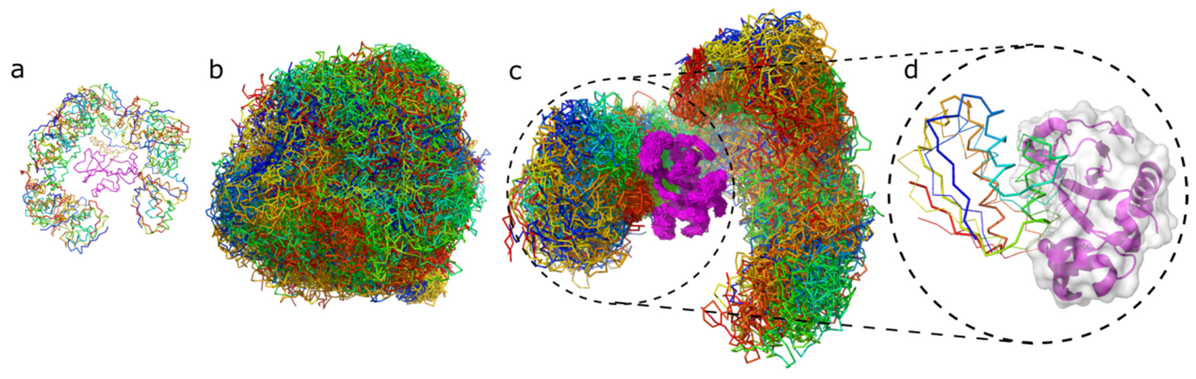
- Generating starting structures. Starting conformations are built using C-alpha coordinates only (in the CABS model C-alpha traces define the position of other united pseudo-atoms, see details [29]). The algorithm places the protein-ligand center at 20 random positions around the protein receptor at the approximate distance of 20 Å from the protein receptor’s surface. Next, these protein-ligand systems are used as starting conformations for the 20 replicas in the REMC CABS sampling scheme (each replica starts from a different ligand-receptor arrangement).
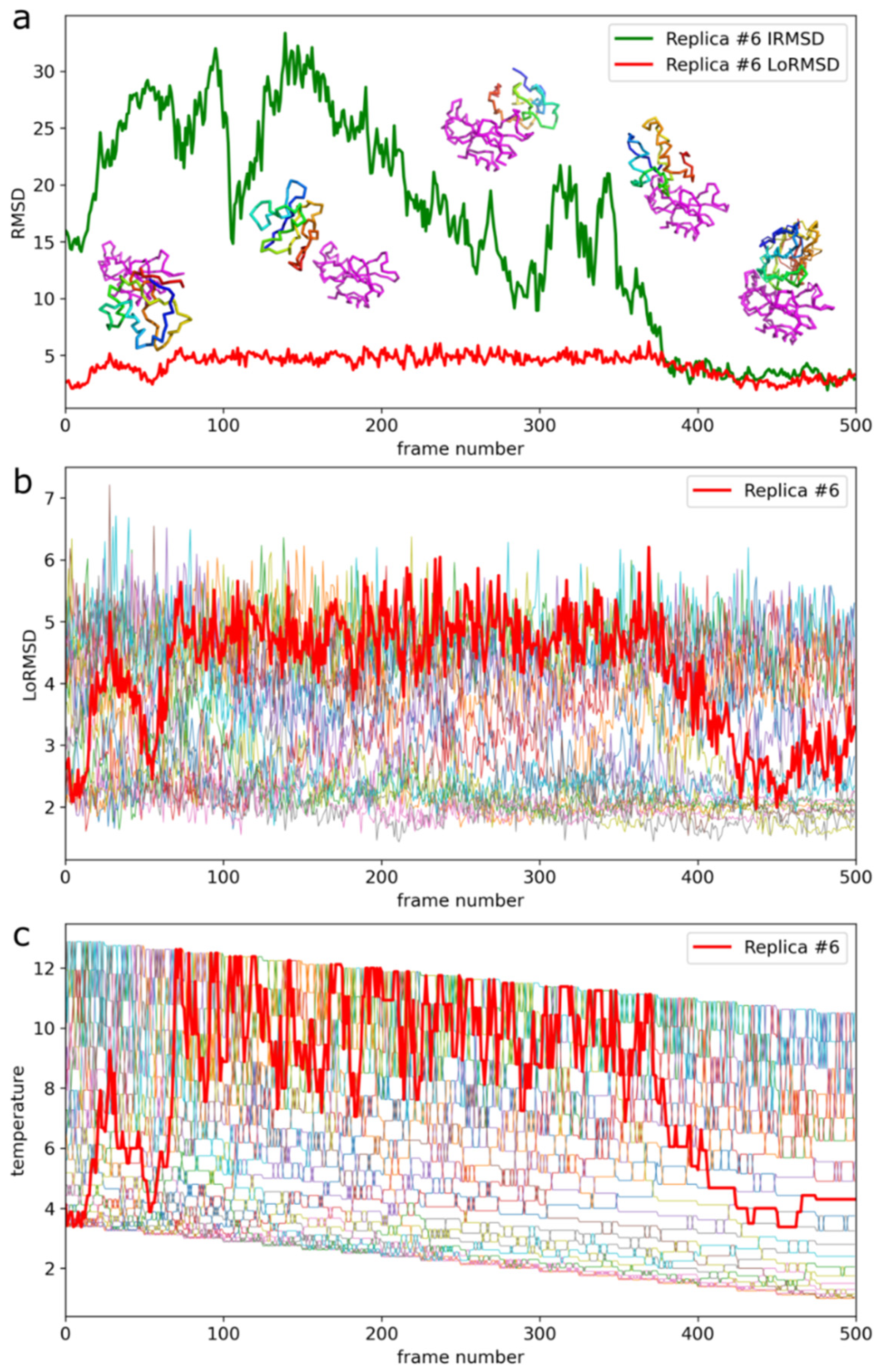
- Docking simulations using CABS coarse-grained model and REMC dynamics. During simulations, the protein receptor structure is kept close to the starting structure using distance restraints. Distance restraints are generated using the input coordinates of the C-alpha atoms. Two residues are automatically restrained if two conditions are met. First, their separation along the sequence has to be at least five residues. Second, the distance between their C-alpha atoms must be within the range of 5–15 Å. During simulations, the receptor restraints imply small-scale fluctuations of the protein receptor backbone in the range of 1 Å and, accordingly, more significant fluctuations of the side-chain atoms. A similar restraints scheme is applied to the protein-ligand but with tenfold weaker weights. During simulations, the ligand moves freely within the vicinity of the receptor and internal restraint allows for large-scale fluctuations of its structure. Usually, the ligand fluctuations are within the range of 2 and 12 Å to the input structure although folding-unfolding events are possible at highest temperatures. The docking simulation is conducted using CABS REMC pseudo-dynamics with simulated annealing. In this work, 20 replicas and 20 annealing steps have been used. All the REMC scheme parameters have been adjusted to allow for large-scale conformational transitions, rotations, and translations of the protein-ligand in a reasonable computational time. The modeling protocol collects trajectories from all 20 replicas. The protocol saves only a small fraction (2%) of the generated models for further analysis i.e., 500 models from each replica, thus 10,000 models in total.
- Reconstructing to CABS coarse-grained representation. The set of 10,000 models in C-alpha traces are reconstructed to complete CABS model representation using CABS algorithm [29]. In CABS, positions of C-beta and Side-Chain united atoms are defined by the positions of the three consecutive C-alpha atoms and the amino acid identity (the most probable positions from the PDB database are used).
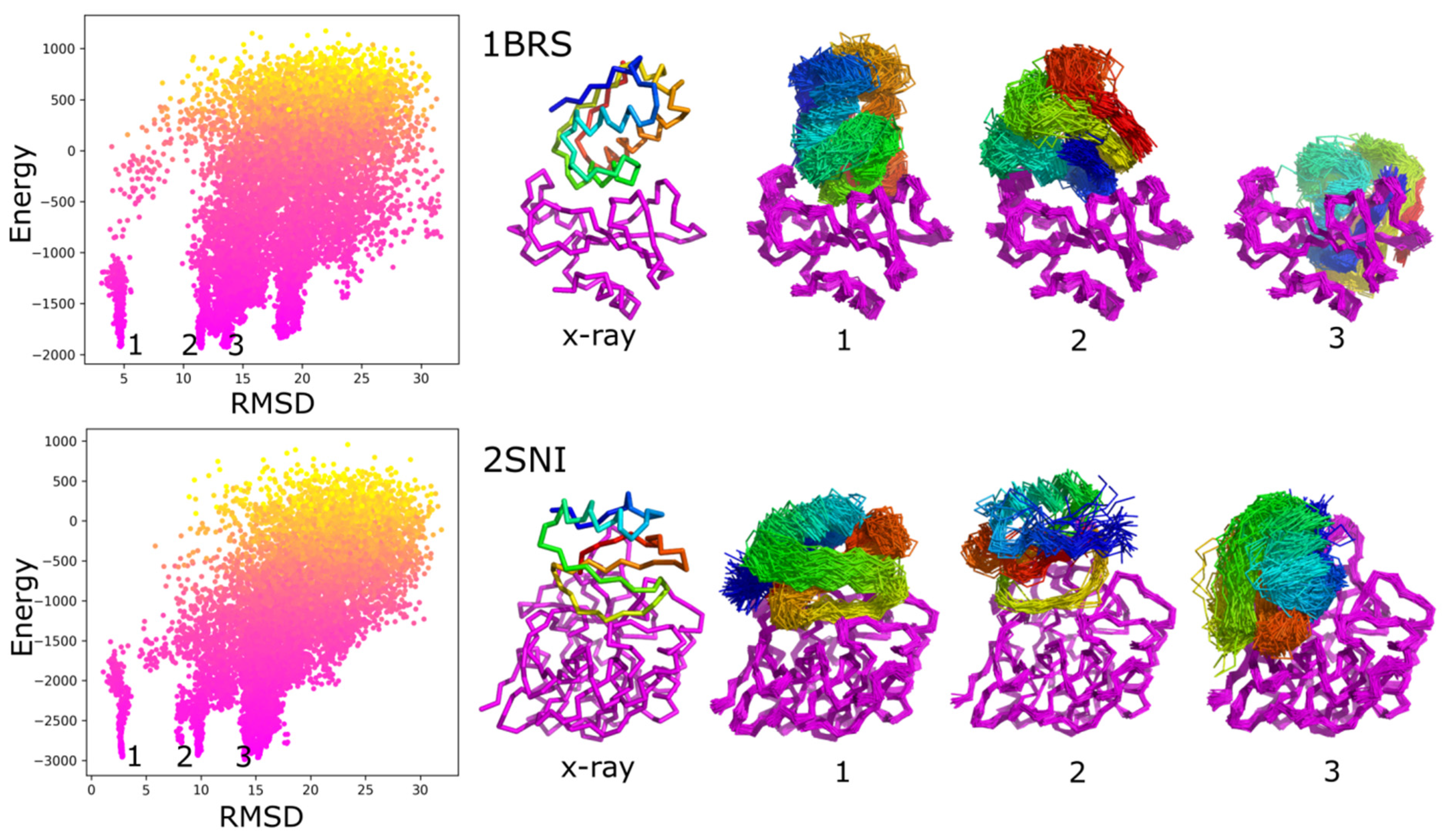
- Clustering of contact maps. First, for all of the 10,000 models the contact maps between the receptor and the ligand proteins are calculated. Two residues are considered to form a contact if their Side Chain pseudoatoms are at most 6 Å apart (for Alanines the C-beta atoms are considered as the Side Chain; for Glycines—it’s the C-alpha atoms). Next, the algorithm sorts the models according to the number of the receptor-ligand contacts, and the set of top 1000 is kept for further processing. This way the transient and weakly bound complexes are removed from the solutions pool. In the next step, the 1000 contact maps are clustered together to identify the most frequently occurring contact patterns. The complete link hierarchical clustering was used with the Jaccard index as the distance metric between contact maps. Finally, the identified clusters are ranked according to their density, defined as the number of the cluster members divided by the average metric between them.
4.2. Results Analysis and Quality Metrics
4.3. Dataset
5. Conclusions
Supplementary Materials
Author Contributions
Funding
Institutional Review Board Statement
Informed Consent Statement
Data Availability Statement
Conflicts of Interest
Correction Statement
References
- Porter, K.A.; Desta, I.; Kozakov, D.; Vajda, S. What method to use for protein–protein docking? Curr. Opin. Struct. Biol. 2019, 55, 1–7. [Google Scholar] [CrossRef]
- Rosell, M.; Fernández-Recio, J. Docking approaches for modeling multi-molecular assemblies. Curr. Opin. Struct. Biol. 2020, 64, 59–65. [Google Scholar] [CrossRef]
- Lensink, M.F.; Velankar, S.; Kryshtafovych, A.; Huang, S.; Schneidman-Duhovny, D.; Sali, A.; Segura, J.; Fernandez-Fuentes, N.; Viswanath, S.; Elber, R.; et al. Prediction of homoprotein and heteroprotein complexes by protein docking and template-based modeling: A CASP-CAPRI experiment. Proteins Struct. Funct. Bioinf. 2016, 84, 323–348. [Google Scholar] [CrossRef] [PubMed]
- Lensink, M.F.; Velankar, S.; Wodak, S.J. Modeling protein–protein and protein–peptide complexes: CAPRI 6th edition. Proteins Struct. Funct. Bioinf. 2017, 85, 359–377. [Google Scholar] [CrossRef] [PubMed]
- Lensink, M.F.; Nadzirin, N.; Velankar, S.; Wodak, S.J. Modeling protein-protein, protein-peptide, and protein-oligosaccharide complexes: CAPRI 7th edition. Proteins Struct. Funct. Bioinf. 2020, 88, 916–938. [Google Scholar] [CrossRef] [PubMed]
- Pierce, B.G.; Wiehe, K.; Hwang, H.; Kim, B.-H.; Vreven, T.; Weng, Z. ZDOCK server: Interactive docking prediction of protein-protein complexes and symmetric multimers. Bioinformatics 2014, 30, 1771–1773. [Google Scholar] [CrossRef] [PubMed]
- Kozakov, D.; Hall, D.R.; Xia, B.; Porter, K.A.; Padhorny, D.; Yueh, C.; Beglov, D.; Vajda, S. The ClusPro web server for protein–protein docking. Nat. Protoc. 2017, 12, 255–278. [Google Scholar] [CrossRef] [PubMed]
- Yan, Y.; Tao, H.; He, J.; Huang, S.-Y. The HDOCK server for integrated protein–protein docking. Nat. Protoc. 2020, 15, 1829–1852. [Google Scholar] [CrossRef] [PubMed]
- Venkatraman, V.; Yang, Y.D.; Sael, L.; Kihara, D. Protein-protein docking using region-based 3D Zernike descriptors. BMC Bioinf. 2009, 10, 407. [Google Scholar] [CrossRef] [PubMed]
- Christoffer, C.; Terashi, G.; Shin, W.; Aderinwale, T.; Maddhuri Venkata Subramaniya, S.R.; Peterson, L.; Verburgt, J.; Kihara, D. Performance and enhancement of the LZerD protein assembly pipeline in CAPRI 38-46. Proteins Struct. Funct. Bioinf. 2020, 88, 948–961. [Google Scholar] [CrossRef]
- Estrin, M.; Wolfson, H.J. SnapDock—template-based docking by Geometric Hashing. Bioinformatics 2017, 33, i30–i36. [Google Scholar] [CrossRef]
- Gromiha, M.M.; Yugandhar, K.; Jemimah, S. Protein–protein interactions: Scoring schemes and binding affinity. Curr. Opin. Struct. Biol. 2017, 44, 31–38. [Google Scholar] [CrossRef]
- Feng, T.; Chen, F.; Kang, Y.; Sun, H.; Liu, H.; Li, D.; Zhu, F.; Hou, T. HawkRank: A new scoring function for protein–protein docking based on weighted energy terms. J. Cheminform. 2017, 9, 66. [Google Scholar] [CrossRef] [PubMed]
- Geng, C.; Jung, Y.; Renaud, N.; Honavar, V.; Bonvin, A.M.J.J.; Xue, L.C. iScore: A novel graph kernel-based function for scoring protein–protein docking models. Bioinformatics 2020, 36, 112–121. [Google Scholar] [CrossRef] [PubMed]
- Yan, Y.; Huang, S.-Y. Pushing the accuracy limit of shape complementarity for protein-protein docking. BMC Bioinf. 2019, 20, 696. [Google Scholar] [CrossRef]
- Siebenmorgen, T.; Zacharias, M. Evaluation of Predicted Protein–Protein Complexes by Binding Free Energy Simulations. J. Chem. Theory Comput. 2019, 15, 2071–2086. [Google Scholar] [CrossRef]
- van Zundert, G.C.P.; Rodrigues, J.P.G.L.M.; Trellet, M.; Schmitz, C.; Kastritis, P.L.; Karaca, E.; Melquiond, A.S.J.; van Dijk, M.; de Vries, S.J.; Bonvin, A.M.J.J. The HADDOCK2.2 Web Server: User-Friendly Integrative Modeling of Biomolecular Complexes. J. Mol. Biol. 2016, 428, 720–725. [Google Scholar] [CrossRef] [PubMed]
- Lensink, M.F.; Brysbaert, G.; Nadzirin, N.; Velankar, S.; Chaleil, R.A.G.; Gerguri, T.; Bates, P.A.; Laine, E.; Carbone, A.; Grudinin, S.; et al. Blind prediction of homo- and hetero-protein complexes: The CASP13-CAPRI experiment. Proteins Struct. Funct. Bioinf. 2019, 87, 1200–1221. [Google Scholar] [CrossRef] [PubMed]
- Harmalkar, A.; Gray, J.J. Advances to tackle backbone flexibility in protein docking. Curr. Opin. Struct. Biol. 2021, 67, 178–186. [Google Scholar] [CrossRef] [PubMed]
- Siebenmorgen, T.; Engelhard, M.; Zacharias, M. Prediction of protein–protein complexes using replica exchange with repulsive scaling. J. Comput. Chem. 2020, 41, 1436–1447. [Google Scholar] [CrossRef]
- Park, T.; Woo, H.; Baek, M.; Yang, J.; Seok, C. Structure prediction of biological assemblies using GALAXY in CAPRI rounds 38-45. Proteins Struct. Funct. Bioinf. 2020, 88, 1009–1017. [Google Scholar] [CrossRef]
- Zalewski, M.; Kmiecik, S.; Koliński, M. Molecular Dynamics Scoring of Protein–Peptide Models Derived from Coarse-Grained Docking. Molecules 2021, 26, 3293. [Google Scholar] [CrossRef]
- Peterson, L.X.; Kang, X.; Kihara, D. Assessment of protein side-chain conformation prediction methods in different residue environments. Proteins Struct. Funct. Bioinf. 2014, 82, 1971–1984. [Google Scholar] [CrossRef] [PubMed]
- Kmiecik, S.; Kouza, M.; Badaczewska-Dawid, A.; Kloczkowski, A.; Kolinski, A. Modeling of Protein Structural Flexibility and Large-Scale Dynamics: Coarse-Grained Simulations and Elastic Network Models. Int. J. Mol. Sci. 2018, 19, 3496. [Google Scholar] [CrossRef] [PubMed]
- Torchala, M.; Gerguri, T.; Chaleil, R.A.G.; Gordon, P.; Russell, F.; Keshani, M.; Bates, P.A. Enhanced sampling of protein conformational states for dynamic cross-docking within the protein-protein docking server SwarmDock. Proteins Struct. Funct. Bioinf. 2020, 88, 962–972. [Google Scholar] [CrossRef]
- Jiménez-García, B.; Roel-Touris, J.; Romero-Durana, M.; Vidal, M.; Jiménez-González, D.; Fernández-Recio, J. LightDock: A new multi-scale approach to protein–protein docking. Bioinformatics 2018, 34, 49–55. [Google Scholar] [CrossRef]
- Kurkcuoglu, Z.; Bonvin, A.M.J.J. Pre- and post-docking sampling of conformational changes using ClustENM and HADDOCK for protein-protein and protein-DNA systems. Proteins Struct. Funct. Bioinf. 2020, 88, 292–306. [Google Scholar] [CrossRef] [PubMed]
- Schindler, C.E.M.; de Vries, S.J.; Zacharias, M. iATTRACT: Simultaneous global and local interface optimization for protein-protein docking refinement. Proteins Struct. Funct. Bioinf. 2015, 83, 248–258. [Google Scholar] [CrossRef] [PubMed]
- Kmiecik, S.; Gront, D.; Kolinski, M.; Wieteska, L.; Dawid, A.E.; Kolinski, A. Coarse-Grained Protein Models and Their Applications. Chem. Rev. 2016, 116, 7898–7936. [Google Scholar] [CrossRef] [PubMed]
- Baaden, M.; Marrink, S.J. Coarse-grain modelling of protein–protein interactions. Curr. Opin. Struct. Biol. 2013, 23, 878–886. [Google Scholar] [CrossRef]
- Roel-Touris, J.; Bonvin, A.M.J.J. Coarse-grained (hybrid) integrative modeling of biomolecular interactions. Comput. Struct. Biotechnol. J. 2020, 18, 1182–1190. [Google Scholar] [CrossRef]
- Krupa, P.; Karczyńska, A.S.; Mozolewska, M.A.; Liwo, A.; Czaplewski, C. UNRES-Dock—protein–protein and peptide–protein docking by coarse-grained replica-exchange MD simulations. Bioinformatics 2020. [Google Scholar] [CrossRef] [PubMed]
- Kuroda, D.; Gray, J.J. Pushing the Backbone in Protein-Protein Docking. Structure 2016, 24, 1821–1829. [Google Scholar] [CrossRef] [PubMed]
- Marze, N.A.; Roy Burman, S.S.; Sheffler, W.; Gray, J.J. Efficient flexible backbone protein–protein docking for challenging targets. Bioinformatics 2018, 34, 3461–3469. [Google Scholar] [CrossRef]
- Roy Burman, S.S.; Nance, M.L.; Jeliazkov, J.R.; Labonte, J.W.; Lubin, J.H.; Biswas, N.; Gray, J.J. Novel sampling strategies and a coarse-grained score function for docking homomers, flexible heteromers, and oligosaccharides using Rosetta in CAPRI rounds 37–45. Proteins Struct. Funct. Bioinf. 2020, 88, 973–985. [Google Scholar] [CrossRef] [PubMed]
- Zacharias, M. ATTRACT: Protein-protein docking in CAPRI using a reduced protein model. Proteins Struct. Funct. Bioinf. 2005, 60, 252–256. [Google Scholar] [CrossRef] [PubMed]
- Glashagen, G.; Vries, S.; Uciechowska-Kaczmarzyk, U.; Samsonov, S.A.; Murail, S.; Tuffery, P.; Zacharias, M. Coarse-grained and atomic resolution biomolecular docking with the ATTRACT approach. Proteins Struct. Funct. Bioinf. 2020, 88, 1018–1028. [Google Scholar] [CrossRef] [PubMed]
- Moal, I.H.; Bates, P.A. SwarmDock and the Use of Normal Modes in Protein-Protein Docking. Int. J. Mol. Sci. 2010, 11, 3623–3648. [Google Scholar] [CrossRef]
- Yan, Y.; He, J.; Feng, Y.; Lin, P.; Tao, H.; Huang, S. Challenges and opportunities of automated protein-protein docking: HDOCK server vs. human predictions in CAPRI Rounds 38-46. Proteins Struct. Funct. Bioinf. 2020, 88, 1055–1069. [Google Scholar] [CrossRef] [PubMed]
- Roel-Touris, J.; Don, C.G.V.; Honorato, R.; Rodrigues, J.P.G.L.M.; Bonvin, A.M.J.J. Less Is More: Coarse-Grained Integrative Modeling of Large Biomolecular Assemblies with HADDOCK. J. Chem. Theory Comput. 2019, 15, 6358–6367. [Google Scholar] [CrossRef]
- Ciemny, M.; Badaczewska-Dawid, A.; Pikuzinska, M.; Kolinski, A.; Kmiecik, S. Modeling of Disordered Protein Structures Using Monte Carlo Simulations and Knowledge-Based Statistical Force Fields. Int. J. Mol. Sci. 2019, 20, 606. [Google Scholar] [CrossRef] [PubMed]
- Badaczewska-Dawid, A.E.; Khramushin, A.; Kolinski, A.; Schueler-Furman, O.; Kmiecik, S. Protocols for All-Atom Reconstruction and High-Resolution Refinement of Protein–Peptide Complex Structures. Methods Mol. Biol. 2020, 2165, 273–287. [Google Scholar] [CrossRef] [PubMed]
- Badaczewska-Dawid, A.E.; Kolinski, A.; Kmiecik, S. Computational reconstruction of atomistic protein structures from coarse-grained models. Comput. Struct. Biotechnol. J. 2020, 18, 162–176. [Google Scholar] [CrossRef] [PubMed]
- Jamroz, M.; Orozco, M.; Kolinski, A.; Kmiecik, S. Consistent View of Protein Fluctuations from All-Atom Molecular Dynamics and Coarse-Grained Dynamics with Knowledge-Based Force-Field. J. Chem. Theory Comput. 2013, 9, 119–125. [Google Scholar] [CrossRef] [PubMed]
- Kuriata, A.; Gierut, A.M.; Oleniecki, T.; Ciemny, M.P.; Kolinski, A.; Kurcinski, M.; Kmiecik, S. CABS-flex 2.0: A web server for fast simulations of flexibility of protein structures. Nucleic Acids Res. 2018, 46, W338–W343. [Google Scholar] [CrossRef] [PubMed]
- Kurcinski, M.; Oleniecki, T.; Ciemny, M.P.; Kuriata, A.; Kolinski, A.; Kmiecik, S. CABS-flex standalone: A simulation environment for fast modeling of protein flexibility. Bioinformatics 2019, 35, 694–695. [Google Scholar] [CrossRef] [PubMed]
- Kmiecik, S.; Gront, D.; Kouza, M.; Kolinski, A. From Coarse-Grained to Atomic-Level Characterization of Protein Dynamics: Transition State for the Folding of B Domain of Protein A. J. Phys. Chem. B 2012, 116, 7026–7032. [Google Scholar] [CrossRef]
- Kmiecik, S.; Kolinski, A. Characterization of protein-folding pathways by reduced-space modeling. Proc. Natl. Acad. Sci. USA 2007, 104, 12330–12335. [Google Scholar] [CrossRef]
- Kmiecik, S.; Kolinski, A. Simulation of Chaperonin Effect on Protein Folding: A Shift from Nucleation–Condensation to Framework Mechanism. J. Am. Chem. Soc. 2011, 133, 10283–10289. [Google Scholar] [CrossRef]
- Kurcinski, M.; Kolinski, A.; Kmiecik, S. Mechanism of Folding and Binding of an Intrinsically Disordered Protein As Revealed by ab Initio Simulations. J. Chem. Theory Comput. 2014, 10, 2224–2231. [Google Scholar] [CrossRef]
- Kurcinski, M.; Jamroz, M.; Blaszczyk, M.; Kolinski, A.; Kmiecik, S. CABS-dock web server for the flexible docking of peptides to proteins without prior knowledge of the binding site. Nucleic Acids Res. 2015, 43, W419–W424. [Google Scholar] [CrossRef]
- Blaszczyk, M.; Kurcinski, M.; Kouza, M.; Wieteska, L.; Debinski, A.; Kolinski, A.; Kmiecik, S. Modeling of protein–peptide interactions using the CABS-dock web server for binding site search and flexible docking. Methods 2016, 93, 72–83. [Google Scholar] [CrossRef]
- Ciemny, M.P.; Kurcinski, M.; Kozak, K.; Kolinski, A.; Kmiecik, S. Highly flexible protein-peptide docking using cabs-dock. Methods Mol. Biol. 2017, 1561, 69–94. [Google Scholar] [CrossRef]
- Kurcinski, M.; Ciemny, M.P.; Oleniecki, T.; Kuriata, A.; Badaczewska-Dawid, A.E.; Kolinski, A.; Kmiecik, S. CABS-dock standalone: A toolbox for flexible protein–peptide docking. Bioinformatics 2019, 35, 4170–4172. [Google Scholar] [CrossRef]
- Blaszczyk, M.; Ciemny, M.P.; Kolinski, A.; Kurcinski, M.; Kmiecik, S. Protein-peptide docking using CABS-dock and contact information. Brief. Bioinf. 2019, 20, 2299–2305. [Google Scholar] [CrossRef]
- Kurcinski, M.; Badaczewska-Dawid, A.; Kolinski, M.; Kolinski, A.; Kmiecik, S. Flexible docking of peptides to proteins using CABS-dock. Protein Sci. 2020, 29, 211–222. [Google Scholar] [CrossRef] [PubMed]
- Ciemny, M.P.; Kurcinski, M.; Blaszczyk, M.; Kolinski, A.; Kmiecik, S. Modeling EphB4-EphrinB2 protein–protein interaction using flexible docking of a short linear motif. Biomed. Eng. Online 2017, 16, 71. [Google Scholar] [CrossRef]
- Ciemny, M.; Kurcinski, M.; Kamel, K.; Kolinski, A.; Alam, N.; Schueler-Furman, O.; Kmiecik, S. Protein–peptide docking: Opportunities and challenges. Drug Discov. Today 2018, 23, 1530–1537. [Google Scholar] [CrossRef] [PubMed]
- Ciemny, M.P.; Debinski, A.; Paczkowska, M.; Kolinski, A.; Kurcinski, M.; Kmiecik, S. Protein-peptide molecular docking with large-scale conformational changes: The p53-MDM2 interaction. Sci. Rep. 2016, 6. [Google Scholar] [CrossRef] [PubMed]
- Badaczewska-Dawid, A.E.; Kmiecik, S.; Koliński, M. Docking of peptides to GPCRs using a combination of CABS-dock with FlexPepDock refinement. Brief. Bioinf. 2020. [Google Scholar] [CrossRef]
- Koliński, M.; Kmiecik, S.; Dec, R.; Piejko, M.; Mak, P.; Dzwolak, W. Docking interactions determine early cleavage events in insulin proteolysis by pepsin: Experiment and simulation. Int. J. Biol. Macromol. 2020, 149, 1151–1160. [Google Scholar] [CrossRef] [PubMed]
- Vreven, T.; Moal, I.H.; Vangone, A.; Pierce, B.G.; Kastritis, P.L.; Torchala, M.; Chaleil, R.; Jiménez-García, B.; Bates, P.A.; Fernandez-Recio, J. Updates to the Integrated Protein-Protein Interaction Benchmarks: Docking Benchmark Version 5 and Affinity Benchmark Version 2. J. Mol. Biol. 2015. [Google Scholar] [CrossRef] [PubMed]


| X-ray Data (Number of Residues) | Ligand Flexibility | Results—Best from All Models | Results—Best from 10 Top-Scored Models | |||||||
|---|---|---|---|---|---|---|---|---|---|---|
| Receptor * | Ligand * | Complex | RMSD ** | Average LoRMSD | iRMSD | LRMSD | fNAT | iRMSD | LRMSD | fNAT |
| Low-flexibility cases | ||||||||||
| 5CHA (238) | 2OVO (53) | 1CHO | 0.62 | 4.84 | 2.65 | 6.95 | 0.48 | 2.96 | 10.93 | 0.18 |
| 2PKA (232) | 6PTI (56) | 2KAI | 0.91 | 4.64 | 3.32 | 11.34 | 0.19 | 4.75 | 15.76 | 0.12 |
| 1CHG (245) | 1HPT (56) | 1CGI | 1.53 | 5.24 | 2.76 | 4.13 | 0.37 | 6.18 | 14.15 | 0.09 |
| 2PTN (223) | 6PTI (58) | 2PTC | 0.31 | 5.23 | 2.97 | 11.86 | 0.29 | 4.39 | 15.93 | 0.15 |
| 1SUP (275) | 2CI2 (64) | 2SNI | 0.37 | 3.89 | 1.09 | 3.86 | 0.69 | 2.81 | 9.09 | 0.46 |
| 2ACE (532) | 1FSC (61) | 1FSS | 0.76 | 4.48 | 3.41 | 7.20 | 0.25 | 15.03 | 32.56 | 0.03 |
| 1MAA (533) | 1FSC (61) | 1MAH | 0.60 | 4.58 | 2.49 | 3.89 | 0.45 | 11.25 | 24.43 | 0.06 |
| 1A2P (108) | 1A19 (89) | 1BRS | 0.47 | 3.33 | 1.94 | 4.19 | 0.64 | 4.01 | 8.74 | 0.14 |
| 1CCP (294) | 1YCC (103) | 2PCC | 0.39 | 4.18 | 3.13 | 10.19 | 0.25 | 11.89 | 26.68 | 0.08 |
| 1SUP (275) | 3SSI (107) | 2SIC | 0.39 | 4.01 | 4.03 | 18.96 | 0.23 | 4.77 | 19.40 | 0.12 |
| 1VFA (223) | 1LZA (129) | 1VFB | 0.59 | 3.72 | 4.61 | 15.07 | 0.11 | 17.45 | 37.15 | 0.00 |
| 1MLB (432) | 1LZA (129) | 1MLC | 0.85 | 3.74 | 2.82 | 10.47 | 0.36 | 8.04 | 33.09 | 0.04 |
| Medium-flexibility cases | ||||||||||
| 1CHG (226) | 1HPT (56) | 1CGI | 2.02 | 5.80 | 2.46 | 3.21 | 0.44 | 5.86 | 10.72 | 0.12 |
| 5C2B (241) | 4ZAI (80) | 5CBA | 1.49 | 4.51 | 2.48 | 7.64 | 0.42 | 9.34 | 16.01 | 0.10 |
| 5P2 (166) | 1LXD (87) | 1LFD | 1.79 | 4.12 | 2.87 | 6.76 | 0.27 | 12.47 | 24.24 | 0.00 |
| 1R6C (142) | 2W9R (97) | 1R6Q | 1.67 | 9.27 | 7.95 | 11.97 | 0.14 | 13.71 | 35.71 | 0.00 |
| 1JXQ (242) | 2OPY (106) | 1NW9 | 1.97 | 4.09 | 7.05 | 8.69 | 0.23 | 9.33 | 17.55 | 0.00 |
| 1IAS (330) | 1D6O (107) | 1B6C | 1.96 | 4.65 | 4.72 | 10.74 | 0.14 | 12.24 | 23.99 | 0.00 |
| 5E56 (116) | 5E03 (113) | 5E5M | 1.56 | 4.16 | 3.83 | 9.09 | 0.23 | 10.96 | 20.00 | 0.00 |
| 2HRA (180) | 2HQT (115) | 2HRK | 2.03 | 7.27 | 3.55 | 10.17 | 0.26 | 10.81 | 32.54 | 0.00 |
| 4BLM (256) | 4M3J (116) | 4M3K | 1.77 | 4.41 | 4.96 | 7.41 | 0.10 | 13.75 | 27.11 | 0.03 |
| 1E78 (578) | 5VNV (120) | 5VNW | 1.49 | 3.81 | 5.93 | 22.23 | 0.10 | 23.89 | 70.83 | 0.00 |
| 3BX8 (167) | 3OSK (121) | 3BX7 | 1.63 | 4.63 | 4.94 | 17.46 | 0.28 | 6.22 | 20.32 | 0.12 |
| 6ETL (124) | 4POY (121) | 4POU | 1.83 | 4.01 | 2.91 | 10.16 | 0.50 | 6.55 | 19.65 | 0.25 |
| 4FUD (246) | 5HDO (126) | 5HGG | 0.84 | 4.22 | 3.59 | 12.52 | 0.19 | 13.00 | 29.3 | 0.00 |
| 3TGR (346) | 3R0M (127) | 3RJQ | 0.79 | 4.00 | 5.32 | 16.98 | 0.13 | 12.77 | 33.94 | 0.00 |
| 6EY5 (585) | 5FWO (129) | 6EY6 | 1.90 | 3.86 | 3.83 | 6.03 | 0.14 | 12.89 | 27.61 | 0.00 |
| 1SZ7 (159) | 2BJN (141) | 2CFH | 1.55 | 5.13 | 1.98 | 4.01 | 0.71 | 2.82 | 5.50 | 0.63 |
| 3V6F (437) | 3KXS (142) | 3V6Z | 1.83 | 7.11 | 6.12 | 16.68 | 0.15 | 6.66 | 20.06 | 0.06 |
| 3CPI (437) | 1G16 (156) | 3CPH | 2.12 | 4.34 | 4.87 | 15.64 | 0.09 | 15.02 | 27.88 | 0.00 |
| 1QJB (460) | 1KUY (166) | 1IB1 | 2.09 | 4.22 | 6.56 | 14.83 | 0.13 | 16.10 | 46.26 | 0.00 |
| 1IAM (185) | 1MQ9 (173) | 1MQ8 | 1.76 | 4.22 | 4.93 | 14.99 | 0.21 | 26.17 | 70.50 | 0.00 |
| 3HI5 (430) | 1MJN (179) | 3HI6 | 1.65 | 3.77 | 5.79 | 23.30 | 0.21 | 19.38 | 49.77 | 0.00 |
| 2G75 (429) | 2GHV (183) | 2DD8 | 2.19 | 5.37 | 5.73 | 13.78 | 0.09 | 17.20 | 34.33 | 0.00 |
| 1A12 (401) | 1QG4 (202) | 1I2M | 2.12 | 4.19 | 2.84 | 6.43 | 0.51 | 3.58 | 6.97 | 0.47 |
| 1N0V (825) | 1XK9 (204) | 1ZM4 | 2.11 | 3.54 | 8.82 | 28.17 | 0.04 | 11.05 | 48.14 | 0.00 |
| 4EBQ (429) | 4E9O (230) | 4ETQ | 0.47 | 3.72 | 7.12 | 14.74 | 0.20 | 8.68 | 19.61 | 0.07 |
| 1S3X (380) | 1XQR (259) | 1XQS | 1.77 | 5.44 | 5.63 | 26.14 | 0.11 | 15.88 | 30.51 | 0.00 |
| 3HEC (329) | 3FYK (282) | 2OZA | 1.89 | 4.29 | 4.35 | 9.32 | 0.33 | 11.24 | 18.8 | 0.03 |
| 6A0X (437) | 2FK0 (322) | 6A0Z | 1.28 | 5.75 | 5.75 | 25.59 | 0.16 | 11.43 | 31.39 | 0.00 |
| Highly flexible cases | ||||||||||
| 1CL0 (316) | 2TIR (108) | 1F6M | 4.9 | 3.83 | 7.02 | 11.34 | 0.10 | 11.92 | 18.06 | 0.00 |
| 1 × 9Y (346) | 1NYC (110) | 1PXV | 2.63 | 4.86 | 5.74 | 14.10 | 0.07 | 7.46 | 16.31 | 0.02 |
| 1JZO (431) | 1JPE (116) | 1JZD | 2.71 | 4.65 | 4.98 | 8.13 | 0.28 | 13.38 | 34.05 | 0.00 |
| 5D7S (423) | 2GMF (121) | 5C7X | 2.26 | 4.17 | 4.12 | 13.61 | 0.34 | 4.69 | 16.74 | 0.20 |
| 1FCH (302) | 1C44 (123) | 2C0L | 2.62 | 5.51 | 5.02 | 5.54 | 0.21 | 10.24 | 24.74 | 0.00 |
| 1YWH (268) | 2I9A (123) | 2I9B | 3.79 | 7.14 | 5.79 | 17.59 | 0.14 | 6.92 | 33.23 | 0.05 |
| 3L88 (550) | 1CKL (126) | 3L89 | 2.51 | 9.86 | 4.83 | 10.90 | 0.17 | 17.84 | 31.87 | 0.00 |
| 1ZM8 (239) | 1J57 (143) | 2O3B | 3.13 | 6.20 | 4.76 | 16.43 | 0.18 | 15.34 | 31.95 | 0.00 |
| 1G0Y (310) | 1ILR (145) | 1IRA | 8.38 | 4.07 | 12.97 | 22.24 | 0.08 | 15.86 | 25.46 | 0.05 |
| 1QUP (219) | 2JCW (153) | 1JK9 | 2.51 | 9.40 | 8.07 | 13.85 | 0.10 | 17.41 | 30.74 | 0.00 |
| 1SYQ (259) | 3MYI (163) | 1RKE | 4.25 | 4.15 | 5.26 | 6.43 | 0.38 | 16.11 | 34.67 | 0.00 |
| 2II0 (463) | 1CTQ (166) | 1BKD | 2.86 | 4.51 | 4.80 | 7.33 | 0.14 | 19.96 | 39.32 | 0.00 |
| 1ERN (416) | 1BUY (166) | 1EER | 2.44 | 5.22 | 12.97 | 13.18 | 0.02 | 17.12 | 30.73 | 0.00 |
| 3AVE (419) | 1FNL (173) | 1E4K | 2.60 | 5.32 | 3.44 | 10.07 | 0.43 | 7.59 | 24.33 | 0.13 |
| 1R8M (195) | 1HUR (180) | 1R8S | 3.73 | 5.50 | 6.67 | 13.41 | 0.09 | 15.15 | 25.10 | 0.00 |
| 1QFK (348) | 1TFH (182) | 1FAK | 6.18 | 5.64 | 8.97 | 15.57 | 0.16 | 15.59 | 34.46 | 0.00 |
| 1F59 (440) | 1QG4 (202) | 1IBR | 2.54 | 5.01 | 6.65 | 14.36 | 0.14 | 16.41 | 33.07 | 0.00 |
| 4DVB (427) | 4DVA (246) | 4DW2 | 2.27 | 3.85 | 6.61 | 21.91 | 0.14 | 9.94 | 29.27 | 0.00 |
| 1NG1 (294) | 2IYL (271) | 2J7P | 2.67 | 4.51 | 8.87 | 18.77 | 0.11 | 18.46 | 48.05 | 0.00 |
| 1UX5 (411) | 2FXU (360) | 1Y64 | 4.69 | 4.15 | 6.42 | 13.50 | 0.27 | 15.50 | 36.42 | 0.00 |
| 1D0N (729) | 1IJJ (371) | 1H1V | 6.62 | 3.44 | 7.92 | 31.14 | 0.36 | 29.12 | 65.07 | 0.03 |
Publisher’s Note: MDPI stays neutral with regard to jurisdictional claims in published maps and institutional affiliations. |
© 2021 by the authors. Licensee MDPI, Basel, Switzerland. This article is an open access article distributed under the terms and conditions of the Creative Commons Attribution (CC BY) license (https://creativecommons.org/licenses/by/4.0/).
Share and Cite
Kurcinski, M.; Kmiecik, S.; Zalewski, M.; Kolinski, A. Protein–Protein Docking with Large-Scale Backbone Flexibility Using Coarse-Grained Monte-Carlo Simulations. Int. J. Mol. Sci. 2021, 22, 7341. https://doi.org/10.3390/ijms22147341
Kurcinski M, Kmiecik S, Zalewski M, Kolinski A. Protein–Protein Docking with Large-Scale Backbone Flexibility Using Coarse-Grained Monte-Carlo Simulations. International Journal of Molecular Sciences. 2021; 22(14):7341. https://doi.org/10.3390/ijms22147341
Chicago/Turabian StyleKurcinski, Mateusz, Sebastian Kmiecik, Mateusz Zalewski, and Andrzej Kolinski. 2021. "Protein–Protein Docking with Large-Scale Backbone Flexibility Using Coarse-Grained Monte-Carlo Simulations" International Journal of Molecular Sciences 22, no. 14: 7341. https://doi.org/10.3390/ijms22147341
APA StyleKurcinski, M., Kmiecik, S., Zalewski, M., & Kolinski, A. (2021). Protein–Protein Docking with Large-Scale Backbone Flexibility Using Coarse-Grained Monte-Carlo Simulations. International Journal of Molecular Sciences, 22(14), 7341. https://doi.org/10.3390/ijms22147341