Considering the numerous applications of disorder prediction, it would be advantageous if a disorder predictor could make predictions in a timely manner (
i.e., a matter of seconds). Such an approach could then easily be applied to studies on the genomic scale. To ensure fast predictions, the input to the method would need to consist of the protein sequence (
i.e., sequence only) and would not make use of sequence-derived information obtained, for example through a search of a sequence database using PSI-BLAST. Some sequence-only approaches have been derived and tested (e.g., ESpritz [
7]) and are typically not as accurate as those methods that make use of additional sequence-derived information. Here, utilizing recent developments in the machine learning community that produce more robust and generalizable models, a new sequence-only protein disorder predictor is developed and evaluated.
2.2.2. Evaluation of WiDNdisorder
Table 1 and
Table 2 show an evaluation of WiDNdisorder with ESpritz [
7], DISOPREDV3 [
10], and DNdisorder [
5]. Of these methods, DNdisorder and DISOPREDV3 make use of additional evolutionary information gathered through a sequence search (e.g., PSI-BLAST [
41]). The added evolutionary information provides a modest increase in performance, but comes at the cost of executing the search for homologous proteins. The values are reported for ESpritz, which does not use evolutionary information. DNdisorder was also included in the evaluation, since it is also based on deep networks. The evaluation metrics used include balanced accuracy, F-measure, Sw and area under the ROC curve. These metrics have been used extensively in the literature [
5,
7,
11,
42] and used in the official CASP assessments [
43,
44], and a complete description of the evaluation metrics and associated formulas can be found in
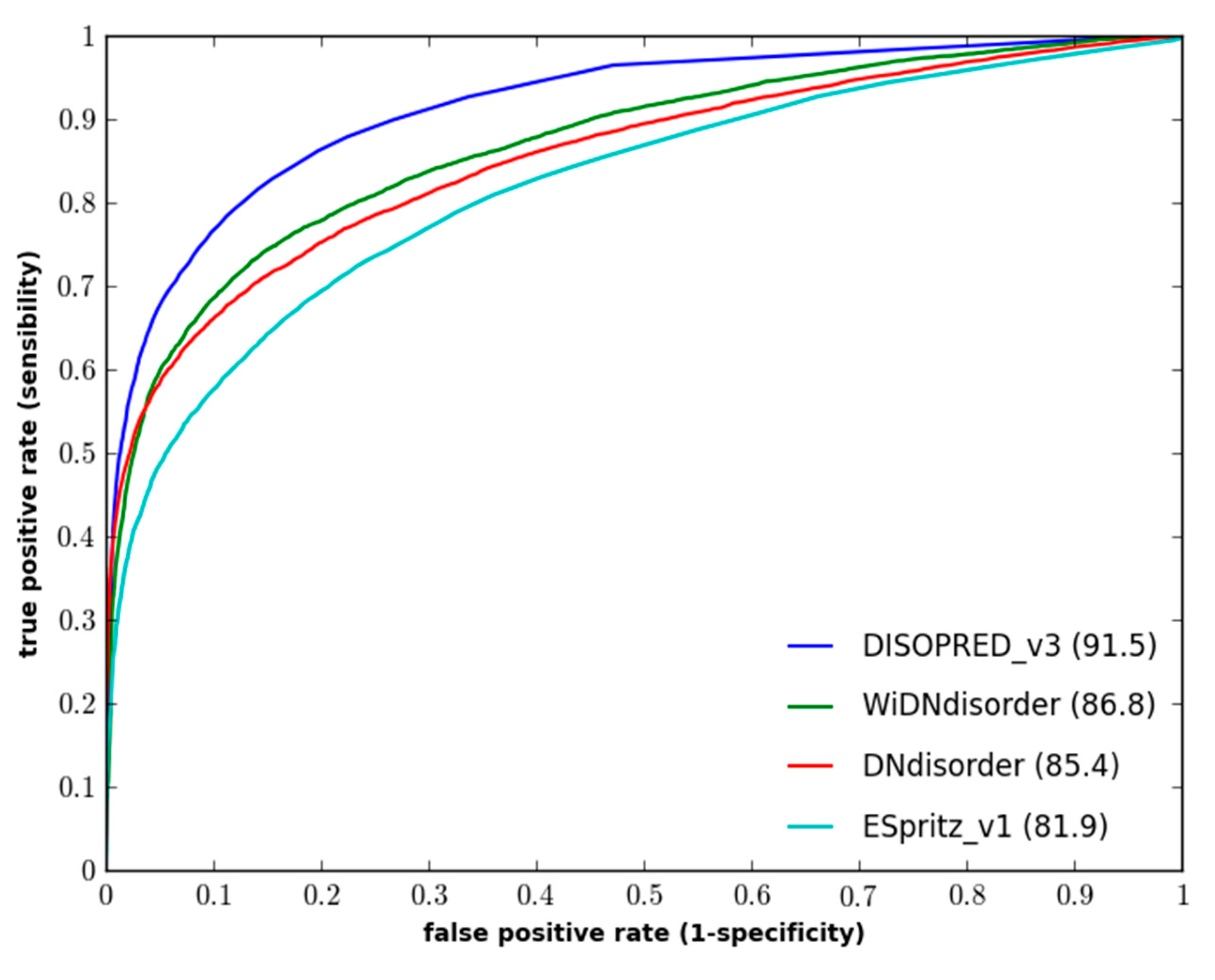
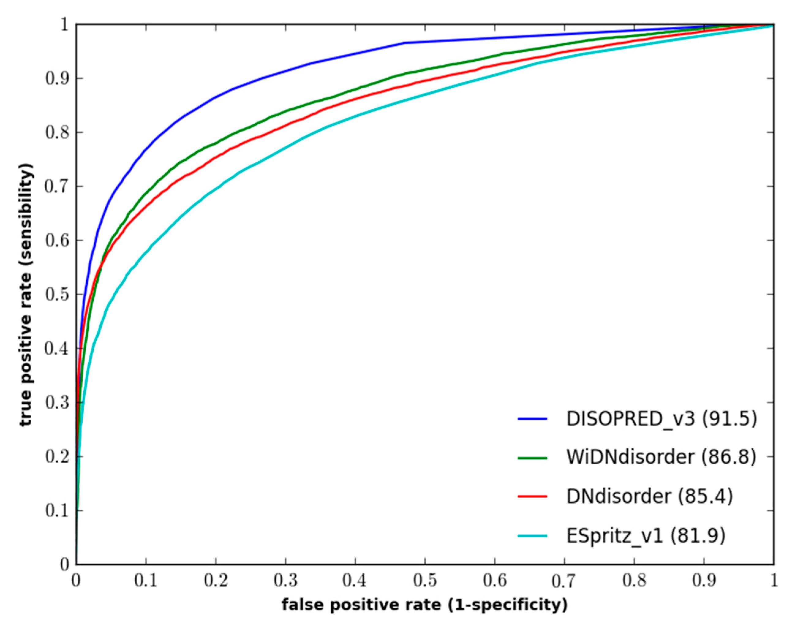
Section 3.3. In terms of balanced accuracy (BAC), WiDNdisorder performed quite well on two independent evaluation datasets. With respect to area under the ROC curve (AUC), WiDNdisorder also performed well, outpacing its principle competitor ESpritz and nearing the performance of DISOPREDV3 on the DO1111_TEST dataset.
Figure 1 and
Figure 2 show the ROC curves for the methods on both evaluation datasets.
Table 1.
Performance of WiDNdisorder (wide deep network disorder predictor) on the DO1111_TEST dataset.
Table 1.
Performance of WiDNdisorder (wide deep network disorder predictor) on the DO1111_TEST dataset.
| Predictor | Balanced Accuracy | F-Measure | Sw | AUC |
|---|
| Value | ±SE | Value | ±SE | Value | ±SE | Value | ±SE |
|---|
| WiDNdisorder | 79.6 | 0.8 | 67.8 | 3.9 | 59.2 | 1.5 | 86.8 | 0.26 |
| ESpritz (v1.3) | 73.8 | 0.4 | 60.8 | 1.8 | 47.5 | 0.79 | 81.9 | 0.30 |
| DISOPRED (v3) | 76.8 | 0.4 | 68.7 | 4.7 | 53.7 | 0.81 | 91.5 | 0.22 |
| DNdisorder | 77.6 | 0.9 | 67.3 | 0.7 | 55.2 | 1.7 | 85.4 | 0.27 |
Table 2.
Performance of WiDNdisorder on the CASP10 dataset.
Table 2.
Performance of WiDNdisorder on the CASP10 dataset.
| Predictor | Balanced Accuracy | F-Measure | Sw | AUC |
|---|
| Value | ±SE | Value | ±SE | Value | ±SE | Value | ±SE |
|---|
| WiDNdisorder | 71.7 | 0.8 | 33.8 | 1.2 | 43.3 | 1.5 | 80.9 | 0.63 |
| ESpritz (v1.3) | 72.0 | 0.8 | 38.7 | 2.1 | 43.8 | 1.6 | 81.3 | 0.64 |
| PrDOS-CNF | 69.4 | 0.8 | 51.2 | 1.4 | 38.7 | 1.7 | 88.3 | 0.53 |
| DISOPRED (v3) | 69.0 | 0.9 | 52.0 | 1.8 | 38.0 | 2.0 | 87.2 | 0.55 |
| DNdisorder | 73.1 | 1.0 | 34.4 | 0.9 | 46.2 | 1.9 | 82.3 | 0.62 |
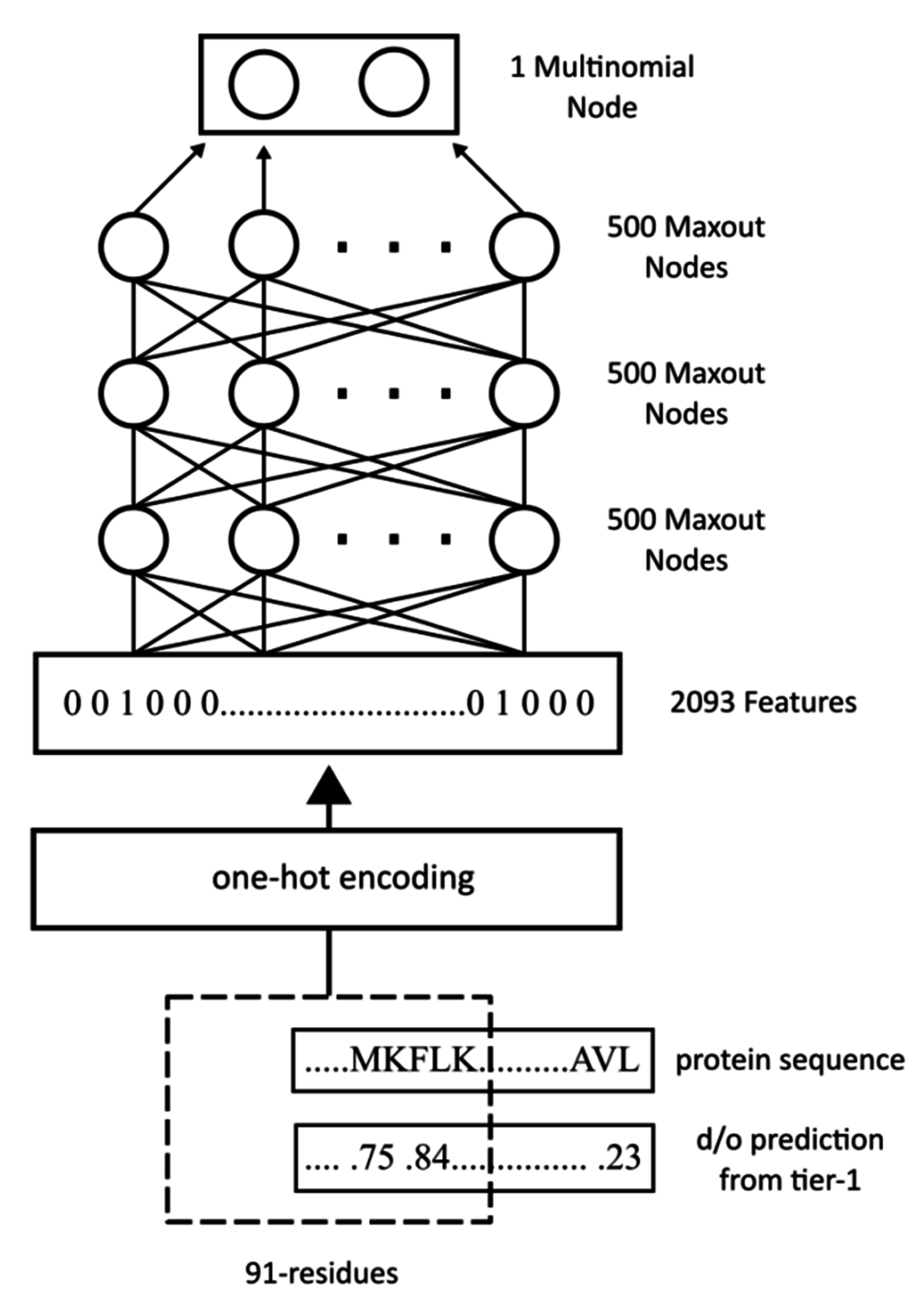
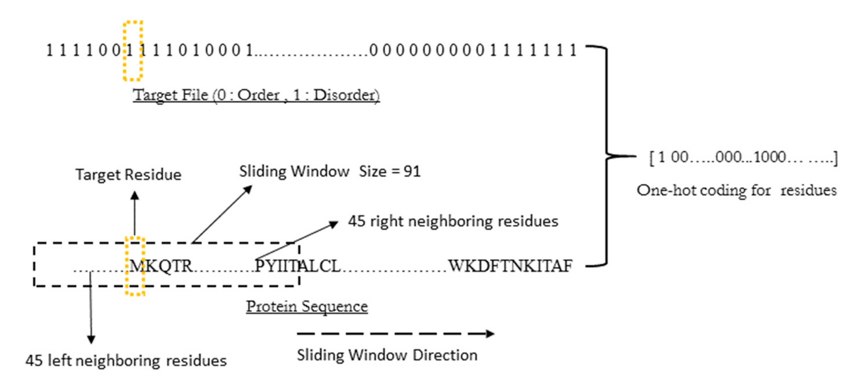
WiDNdisorder makes order/disorder predictions through a two-stage process. In the first stage (
i.e., Tier 1), order/disorder predictions are made for each residue from the protein’s primary sequence, and in the second stage (Tier 2), the initial prediction is refined using the predicted order/disorder state of neighboring residues as additional input to the prediction process.
Table 3 shows the results of a comparison of WiDNdisorder (
i.e., Tier 2/refined predictions)
versus the unrefined predictions generated from one wide deep network (
i.e., Tier 1 predictions) on both evaluation datasets. This indicates the value of the two-stage prediction approach used by WiDNdisorder. For full details on the distinction between Tier 2 and Tier 1 predictions, consult
Section 3.1 and the accompanying figures.
Figure 1.
Performance of disorder prediction methods on the DO1111_TEST dataset.
Figure 1.
Performance of disorder prediction methods on the DO1111_TEST dataset.
Figure 2.
Performance of disordered prediction methods on the CASP10 dataset.
Figure 2.
Performance of disordered prediction methods on the CASP10 dataset.
Table 3.
Comparison of Tier 1 and Tier 2 predictions from WiDNdisorder on the DO1111_TEST and CASP10 datasets.
Table 3.
Comparison of Tier 1 and Tier 2 predictions from WiDNdisorder on the DO1111_TEST and CASP10 datasets.
| Dataset | Tier-1 | Tier-2 |
|---|
| AUC | ±SE | AUC | ±SE |
|---|
| DO1111_TEST | 84.1 | 0.28 | 86.8 | 0.26 |
| CASP10 | 78.8 | 0.65 | 80.9 | 0.63 |
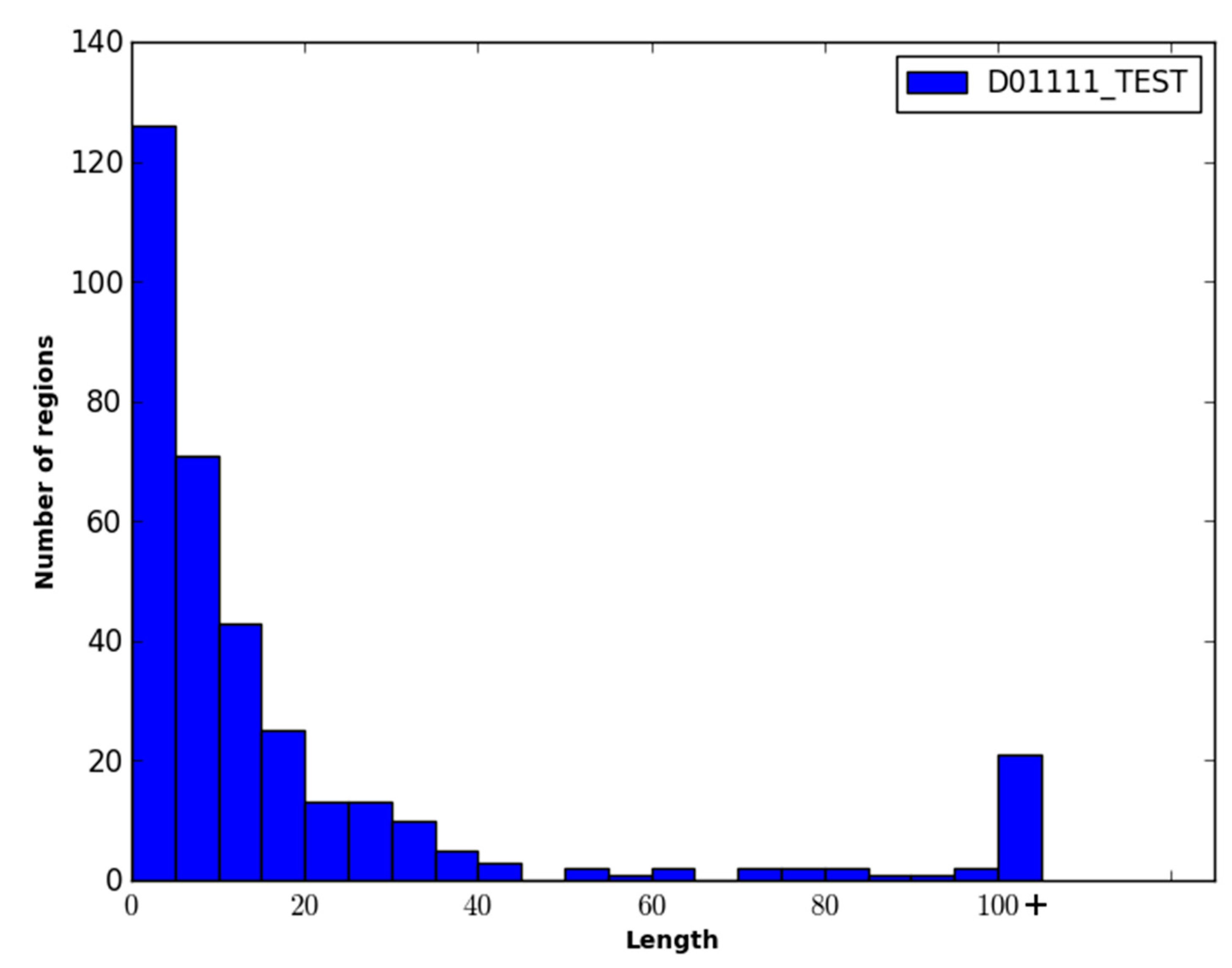
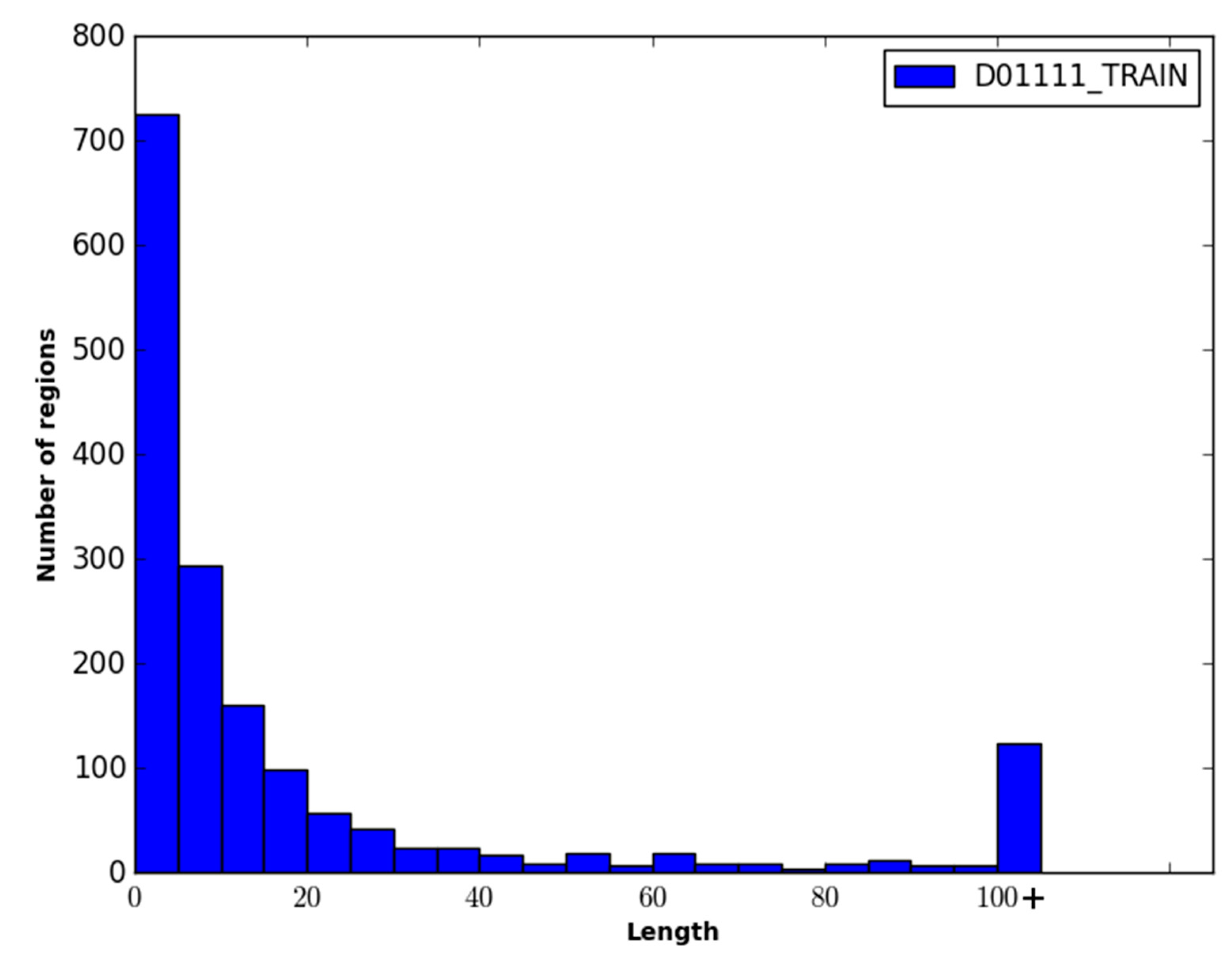
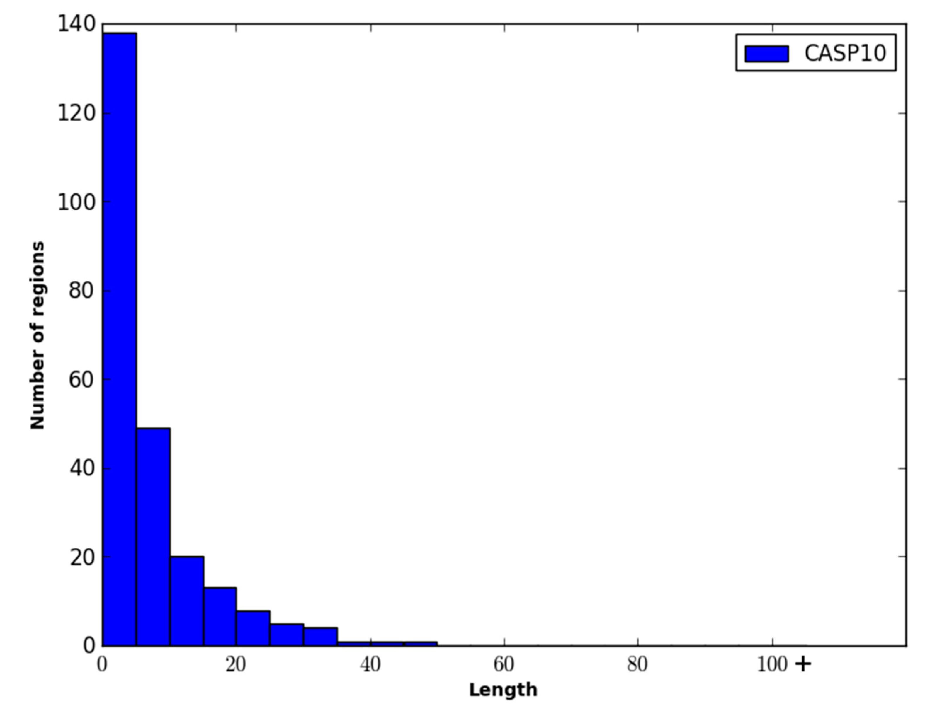
The performance of WiDNdisorder was also evaluated on disordered regions of various lengths. For this evaluation, only residues from contiguous sets of disordered residues of specified ranges were considered, and the percentage of residues correctly predicted to be disordered was determined (
i.e., of the disordered residues in the range considered, what percent were correctly predicted to be disordered). As an example, consider the range 1–5. All order/disorder predictions for residues that pertained to a disorder region in a protein that measured 1–5 residues in length was retained and evaluated.
Table 4 and
Table 5 contain the results of this evaluation for ranges 1–5, 6–15, 16–25 and >25 on the DO1111_TEST and CASP10 datasets. As only disordered residues are considered in this evaluation, the percentage correctly predicted as disordered corresponds to recall.
Table 4.
Recall of disordered predictions by disorder region length on the DO1111_TEST dataset.
Table 4.
Recall of disordered predictions by disorder region length on the DO1111_TEST dataset.
| Predictor | Length of Disordered Region |
|---|
| 1–5 | 6–15 | 16–25 | >25 |
|---|
| WiDNdisorder | 76.2 | 57.9 | 67.2 | 74.3 |
| ESpritz (v1.3) | 74.7 | 63.3 | 67.4 | 55.9 |
| DISOPRED (v3) | 39.2 | 43.3 | 52.2 | 58.5 |
| DNdisorder | 75.4 | 74.1 | 76.1 | 57.9 |
Table 5.
Recall of disordered predictions by disorder region length on the CASP10 dataset.
Table 5.
Recall of disordered predictions by disorder region length on the CASP10 dataset.
| Predictor | Length of Disordered Region |
|---|
| 1–5 | 6–15 | 16–25 | >25 |
|---|
| WiDNdisorder | 57.5 | 60.0 | 57.8 | 50.8 |
| ESpritz (v1.3) | 46.2 | 52.7 | 65.6 | 52.9 |
| PrDOS-CNF | 28.7 | 39.8 | 46.9 | 46.1 |
| DISOPRED (v3) | 25.1 | 33.6 | 49.8 | 47.5 |
| DNdisorder | 48.8 | 64.6 | 66.0 | 53.4 |
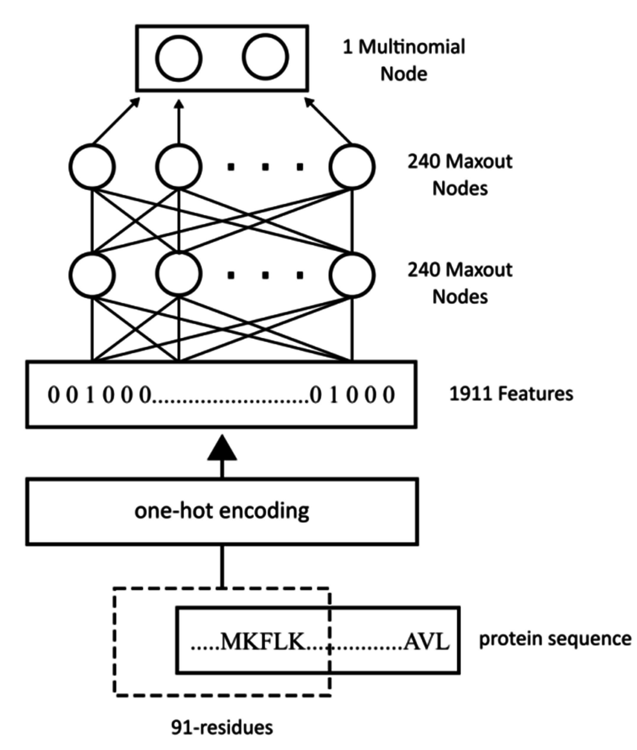
As an initial investigation into the benefit of wide input windows and combinations of dropout and maxout nodes for this particular protein prediction task, a number of disorder predictors were trained for input windows of size 31, 51, 71 and 91. The AUC for each combination of window size and network architecture (
i.e., dropout only, maxout nodes only, dropout with maxout nodes) was calculated for the CASP10 and D01111_TEST datasets, and the results are shown in
Table 6 and
Table 7. Larger input window sizes and the combination of dropout and maxout nodes consistently led to better performance.
Table 6.
AUC for disorder predictions by input window size on the D01111_TEST dataset.
Table 6.
AUC for disorder predictions by input window size on the D01111_TEST dataset.
| Deep Network Configuration | Input Window Size (in Residues) |
|---|
| 31 | 51 | 71 | 91 |
|---|
| dropout only | 78.6 | 81.6 | 82.6 | 83.3 |
| maxout nodes only | 78.0 | 79.2 | 80.8 | 80.9 |
| maxout nodes with dropout | 81.7 | 83.3 | 83.7 | 84.1 |
Table 7.
AUC for disorder predictions by input window size on the CASP10 dataset.
Table 7.
AUC for disorder predictions by input window size on the CASP10 dataset.
| Deep Network Configuration | Input Window Size (in Residues) |
|---|
| 31 | 51 | 71 | 91 |
|---|
| dropout only | 71.0 | 70.0 | 73.0 | 74.9 |
| maxout nodes only | 71.3 | 73.0 | 74.7 | 75.8 |
| maxout nodes with dropout | 76.7 | 77.7 | 78.4 | 78.8 |
Finally, to evaluate the speed at which WiDNdisorder is capable of executing, the time required to predict the ordered/disordered state of each residue in a protein was calculated using the time command (i.e., a built-in command available in a Linux command line environment that can determine the execution time of a program). A prediction script was created, which took as input a FASTA file for a protein, predicted the ordered/disordered score for each residue in the protein and then saved the results to a file. The time command was used in conjunction with the prediction script to calculate the entire time needed make predictions for each individual protein in the evaluation datasets. The average execution time needed to make ordered/disordered predictions for a protein was 7.86 and 7.19 seconds on the DO1111_TEST and CASP10 datasets, respectively.


