Previously, we considered interactions involving angular momentum [
7]. Here, we introduce an angular coordinate interaction potential that will determine the floppiness of two rotors. A two-rotors model is sketched in
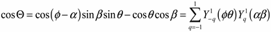
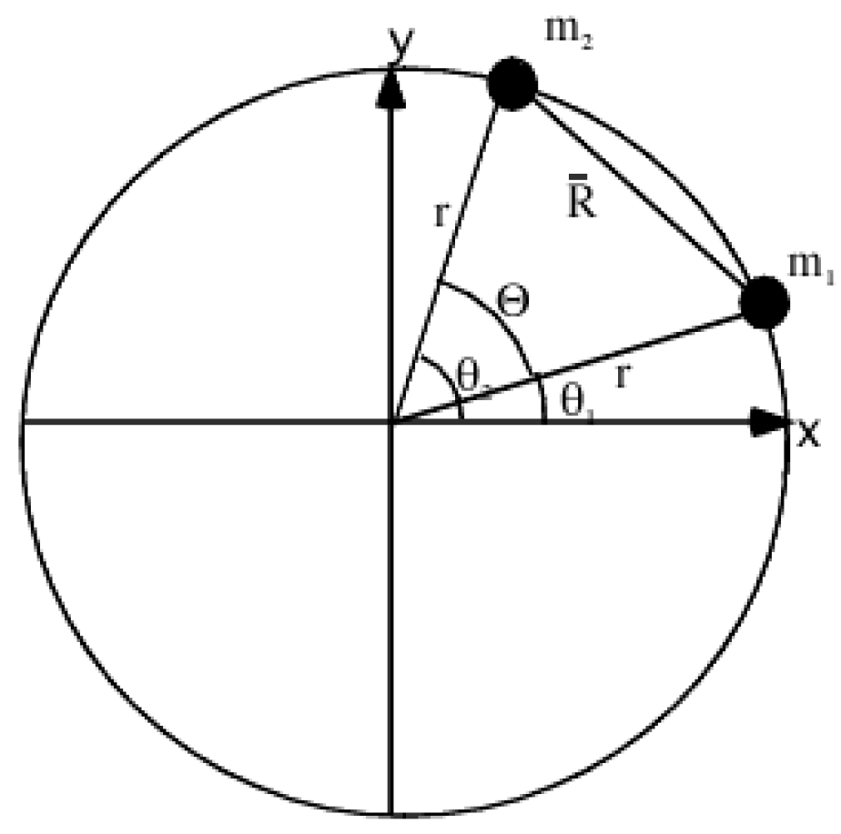
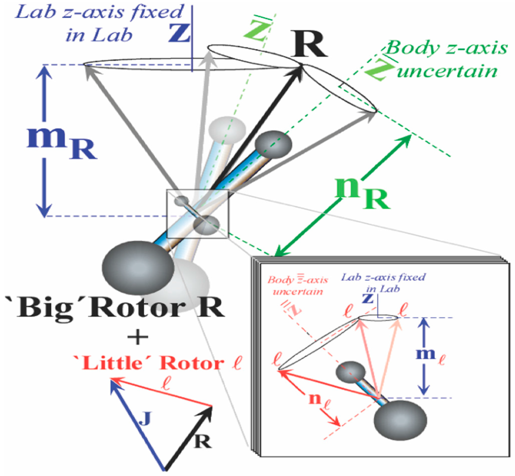
Figure 1. Before coupling we imagine that a “big” rotor R is oriented at some angle β relative to the lab while the other “little” rotor axis is oriented at lab polar angle θ, and the angle Θ lies between them (if the two were in the same plane with Θ = β ± θ as shown in [
7,
8,
9,
10]). We use R to designate the “big” rotor momentum quanta, while
ℓ designates that of the “little” or “faster” rotor. (The formalism must be adapted to the rotor being identical as well as to having the R rotor being “faster or smaller”).
Figure 1.
Schematic of coupled rotor system taken from [
7]. The angular momentum
J,
R, and
ℓ are shown along with their projection of the lab and body axis.
We consider a model such that the two rotors are connected to each other by a spring. We use Equation (1) to show a simple way to model this behavior.
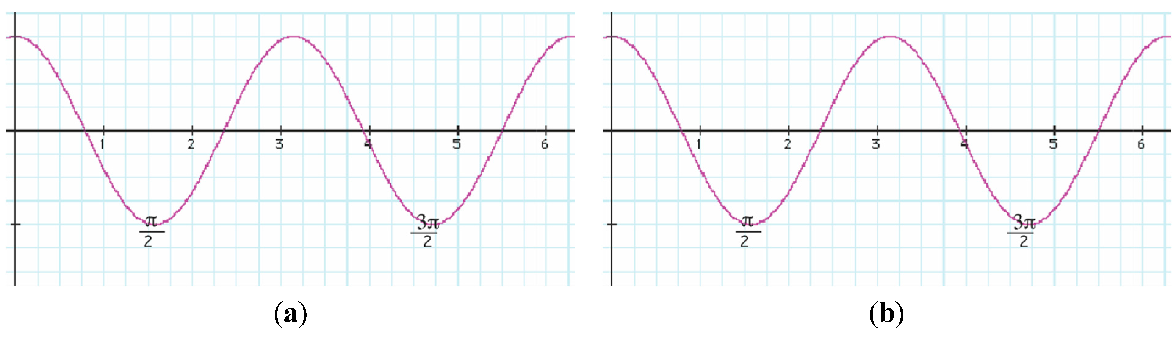
Figure 2.
The graph of cosnΘ (a) n = 2 and (b) n = 3.
The general procedure is to diagonalize the Hamiltonian for the rotor–rotor interaction at the different coupling strengths and then weave our way through the energy spectrum looking for the regions of a composite rotor’s top behavior.
To illustrate the behavior of our coupling Hamiltonian we will now consider the case where two diatomic molecules are coupled together.
2.1. Example: Coupling between Two Diatomic Molecules X2 with n = 2
Let us consider two X
2 rotors interacting through a periodic potential as given by Equation (5).
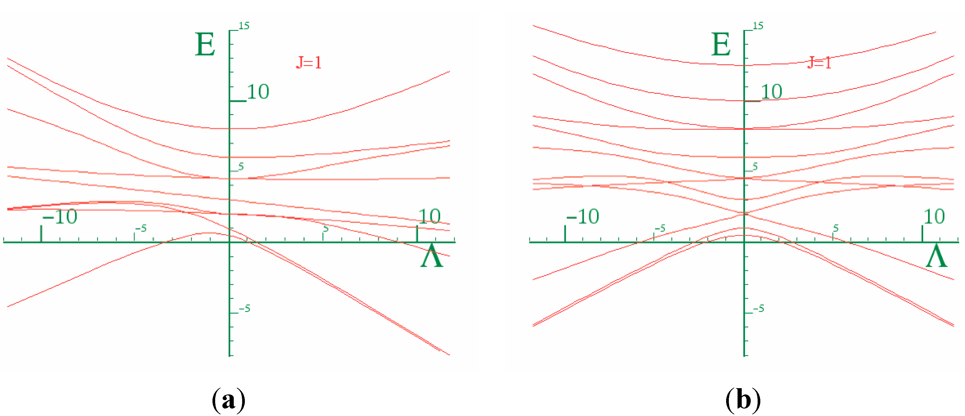
Figure 3a,b shows the energy E
vs. the coupling constant Λ. We choose B = 0.5 kg·m
−2 as the rotational constant to approximate that of H
2 given in [
21] for
![Ijms 15 19662 i014]()
. This value was rescaled by a factor of 10 on the plot. The plots of
Figure 3a,b correspond to the interaction potential in
Figure 2 with
n = 2 and 3 respectively.
We know that all three angular momenta are good quantum numbers in the LWC basis. However, in the BOA basis only angular momenta
ℓ and
J remain so whereas, for higher terms in the multi-pole expansion, the
ℓ quantum becomes uncertain and the higher
ℓ states must be coupled according to Equation (8b). As a result,
ℓ will not be a good quantum number even though J is always conserved in the absence of external forces. To achieve conservation, the angle between the two rotors is more nearly conserved with the higher powers of the cosine.
Figure 3 shows that as we increase the power of cosine, there is mixing of higher
ℓ levels. Due to lab symmetry (absence of external torque) the matrix for Equation (8) is a block diagonal in
J due to the conservation of total angular momentum. However, there is a multipolarity-k-dependent mixing of the levels and
ℓ that is not conserved. Physically, the vibration or flopping is reduced and the rotor of angular momentum
ℓ acts like a passenger on the rotor of the angular momentum R with neither
ℓ nor R being constant. When the rotors are locked in together, the only degrees of freedom remaining are those of the individual rotors’ spin
nℓ or
nR about their body axis. A system in which one of the rotors is allowed to move in this fashion is discussed in [
11], and the case where both are allowed to turn is studied in [
22].
Figure 3.
Energy vs. coupling of X2 for J = 1. (a) n = 2; (b) n = 3.
Figure 3.
Energy vs. coupling of X2 for J = 1. (a) n = 2; (b) n = 3.
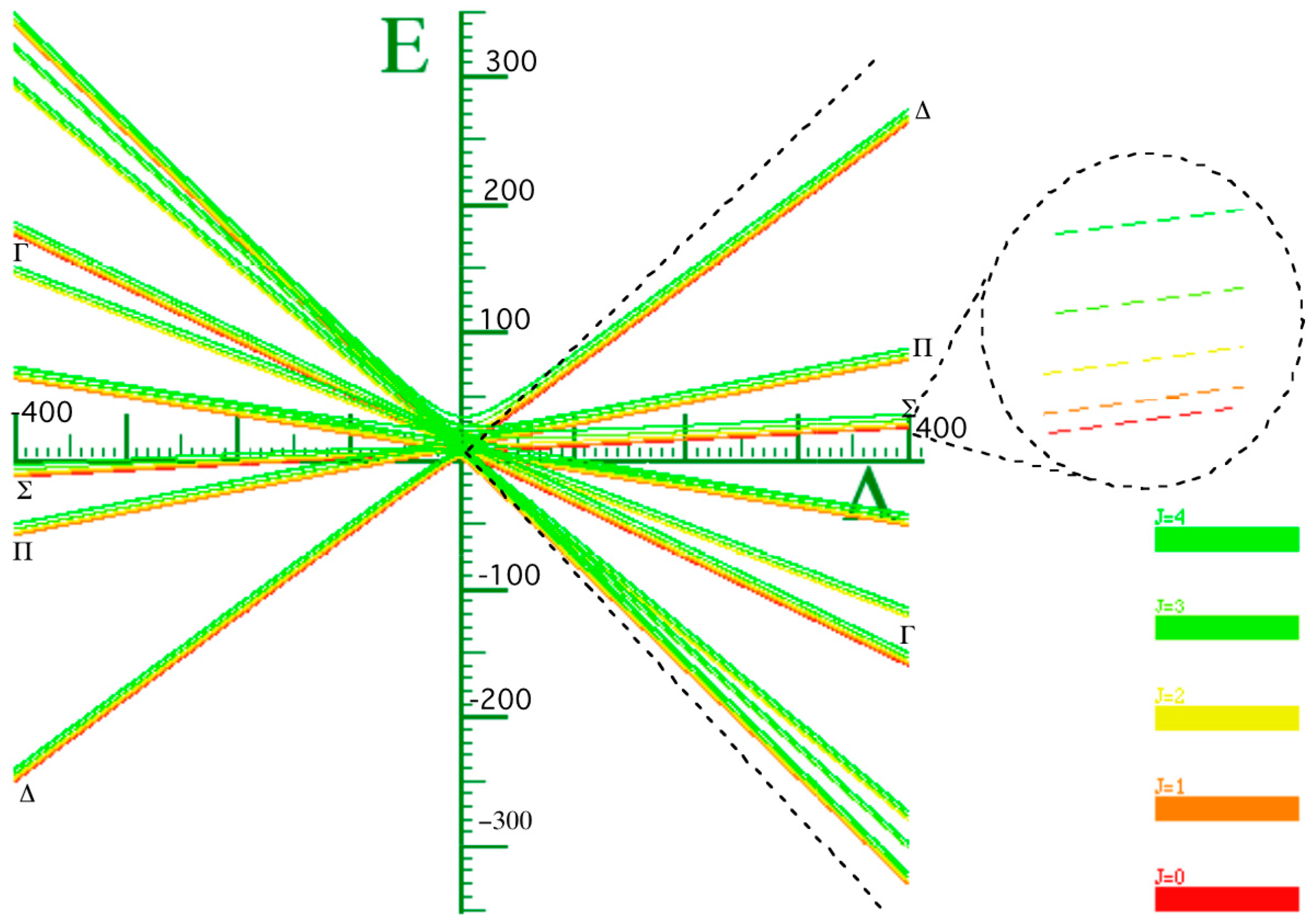
To really make a case for a single composite rotor emerging from this coupled rotor system, we must turn coupling Λ to the highest possible value. In light of
Figure 3 we see that at low coupling of Λ, the eigen-energies are unsettled. As coupling increases, the levels come together to form bands. In
Figure 4, the energy band label (Ʃ) corresponds to the angular momentum values of 0, 1, 2, 3, and 4. The next band of levels (Π) contains only four levels with values 1, 2, 3, and 4. The next band is partly a duplication of the first. The spacing between the energy levels in some of the bands follows the Lande interval rule as presented in
Table 1.
Table 1.
The energy spacing values ∆Ej.
Table 1.
The energy spacing values ∆Ej.
| Ʃ Band | ∆ Band | Γ Band |
|---|
| 1.07784 | 1.0337 | 1.0101 |
| 2.15526 | 2.0675 | 2.0204 |
| 3.2361 | 3.101 | 3.0304 |
| 4.3029 | 4.1348 | 4.04004 |
Figure 4 is a plot of two X
2 molecules interacting through a cosine potential with
n = 2. The inertia coefficient around the
B axis was chosen to be 0.5 kg
−1·m
−2. The coefficient around the
C axis is infinitely large for a diatomic molecule, but this does not contribute to the energy since there is no spin or twist around this axis. The coupled system has an overall B coefficient when it is locked together with 0.5 kg
−1·m
−2. From the Lande interval, we get an overall B coefficient of 0.5 kg
−1·m
−2. In
Table 1, the energy spacing ∆
Ej = Ej − Ej−1 follows the
ℓ interval rule.
Figure 4.
Energy vs. coupling of X2 molecule for J = 1, n = 2.
Figure 4.
Energy vs. coupling of X2 molecule for J = 1, n = 2.
The graph in
Figure 3a is asymmetric while the graph in
Figure 3b displays a greater degree of symmetry. The reason is that when
n = 3 when there are three minima, two at
![Ijms 15 19662 i015]()
(one on either side of Θ =
π) and one at Θ =
π. Therefore, the graph is symmetric at about π. This is a stable point. For
n having odd values, the graphs will be symmetric around π. Thus the two diatomic molecules would prefer aligning parallel to each other at Θ =
π for
N = 3 but have a perpendicular alignment for
![Ijms 15 19662 i016]()
, which corresponds to
N = 2.
The wavefunctions for a free diatomic molecule are the spherical harmonics. We use Clebsch–Gordan’s coefficient to couple two or more diatomic molecules together. A very strong coupling constant would take us to the BOA basis. The BOA wavefunction derived in [
7] is used to describe the coupled system of two diatomic molecules in the strong limit with body quantum number
nℓ = 0 and
nR = 0 required for two diatomic molecules. Thus our BOA wavefunction reduces to the wavefunction described in [
6,
7].
Now, Equation (10) presents the picture of an electron interacting with a bare diatomic rotor molecule [
6]. The BOA basis corresponds to a third body emerging from joining two rotor systems, which can also be seen in our previous work [
7,
8,
9,
10].
Figure 4 of [
9] provides a schematic visual of composite rotor forms in SF
5CF
3, and in
Figure 4,
Figure 5,
Figure 6,
Figure 7,
Figure 8,
Figure 9,
Figure 10 and
Figure 11 of [
8] we are given a visual in the context of rotational energy (RES).
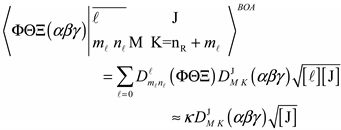
The uncertainty of both R and ℓ angular momenta results in localizing our wavefunction in the BOA basis, which is approximately given by a single wavefunction of total angular momentum J. In other words, the rotors are rigidly connected to each other and are not able to flop around. We coin the term “extremely constricted BOA state” for the situation where the ℓ quantum number becomes uncertain. The following simple sum ℓ constituent is an approximation of the BOA constricted state. Equation (11) reveals the composite rotor as these rotors become extremely constricted.
However, the foregoing analysis constitutes a “shot-gun” wedding of the two rotors by Hamiltonian Equation (6), and it is still unclear whether the marriage is a success. To help our understanding, we turn to simpler models for which the diagonalization is less time consuming.
2.2. Comparative Studies with a 3D-Coupled Rotor System
2.2.1. A Free 1D Rotor Interacting Cosine Potential
We construct a simple model to understand the mechanism by which a single composite rotor emerges from two coupled rotors. A weakly coupled system or floppy system is related to the opposite situation where they are strongly coupled. To begin, we will illustrate the effects of a free rotor in a Mathieu type potential. Angular momentum is transverse to its body axis. The Hamiltonian for a simple one dimensional free rotor system is given by Equation (12).
One may visualize a disk rotating about some imaginary axis perpendicular to the center of the disk. The wavefunction for a state ⎥
m〉 of definite momentum (
m = 0, ±1, …,) in
ℏ-units for such a Hamiltonian is given by Equation (12):
A quasi-quadratic free 1D rotor spectrum results in,
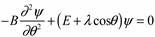
Now with a cosine potential, the Hamiltonian is represented in the Θ angle basis by a Mathieu type Schrödinger Equation (15a):
The solution of Equation (15a) is complicated since simple angular momentum states ⎥m〉 are no longer eigensolutions. Therefore we use a new base in Equation (15b), which is a linear combination of the angular momentum states ⎥m〉.
The matrix representation of the Hamiltonian in the ⎥
m〉 basis is an infinite matrix as given in Equation (16):
The infinite matrix in ⎥m〉 basis may be truncated to a finite set with m ≤ mcutoff in order to diagonalize it to give the energy levels. The results depend on the sensitivity of the coupling constant λ, which determines whether or not the rotor is above the barrier. Whether the rotor in state ⎥εk〉 is stuck or loose depends on its energy level (eigenvalue εk) being above or below the cosine barrier λ.
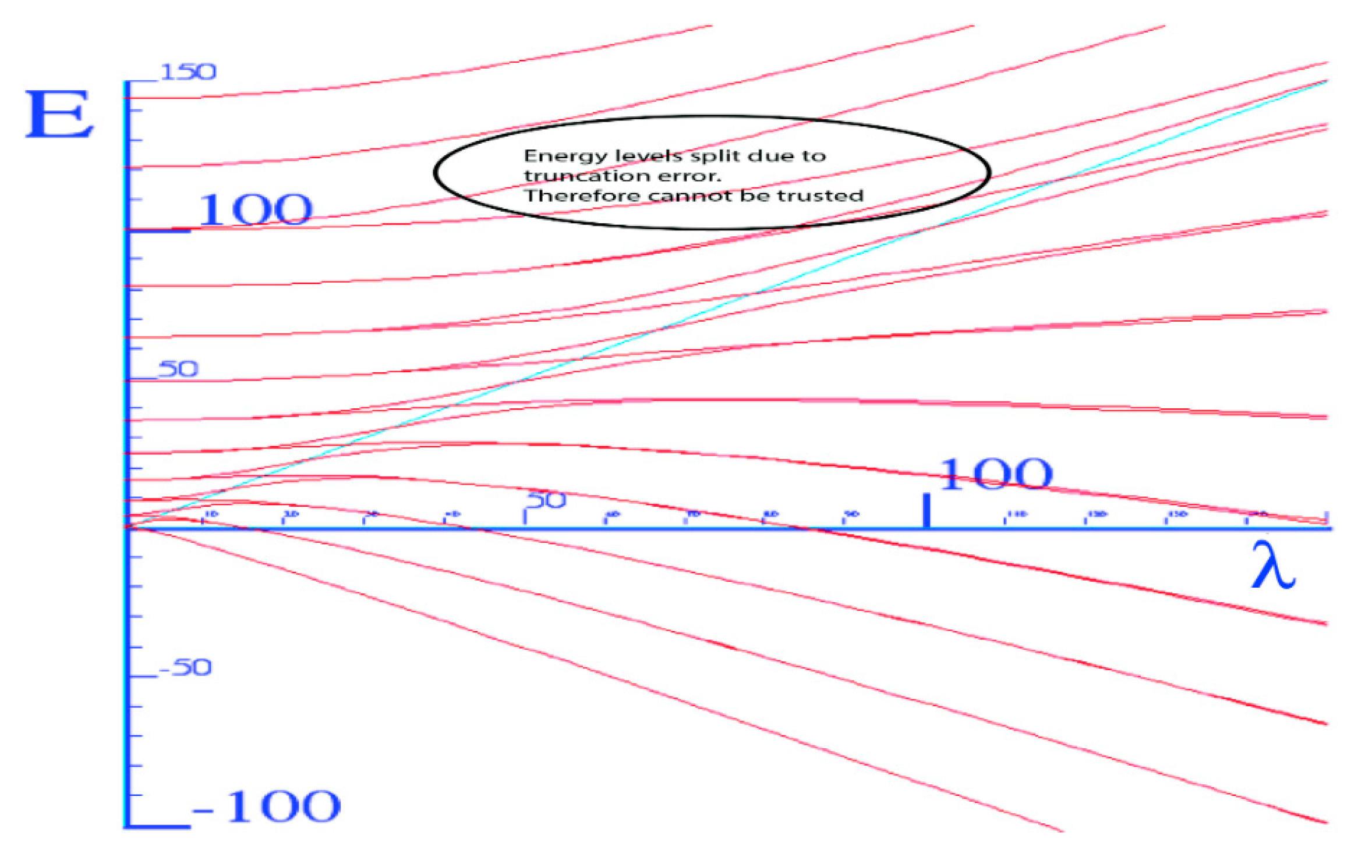
The graph of energy eigenvalues
vs. λ (
Figure 5) shows that above the barrier the spectrum is quasi-quadratic (nearly free rotors) but below, the barrier of the spectrum is quasi-linear (trapped rotors in oscillator potential). The trapped energy levels below the barrier are nearly doubly degenerated because there are two equivalent wells. Near the barrier, the levels split and recombine with other levels to eventually form doubly degenerated quasi-free rotor levels above the barrier.
Figure 5.
Energy vs. coupling for the Mathieu (truncation errors above E = 100 cm−1).
Figure 5.
Energy vs. coupling for the Mathieu (truncation errors above E = 100 cm−1).
2.2.2. Two 1D Rotors Interacting through Angular Potential
A coupled three-dimensional rotor system is considerably more complicated. However, we can be ingenious about using the insight from the one dimensional Mathieu problem. Suppose that both rotors are constrained to rotate about their body axes normal to a plane in which they both lie as illustrated by (
Figure 6). We can use a classical mechanic description for two particles on rings or two discs rotating about the same axle at different angular speeds. Equations (17)–(20) is the derivation of the Lagrangian for the system in
Figure 6.
Figure 6.
Illustration of two particles moving on a ring.
Figure 6.
Illustration of two particles moving on a ring.
Using the center mass frame we have:
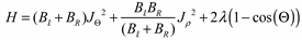
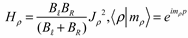
To quantize our system, it is best to represent our model by using a classical Hamiltonian,
which gives:
Our Hamiltonian is in the form of an overall rotation plus the Mathieu equation both of which we have investigated to some degree. Since the angle of the potential between two coupled diatomic rotors has factor 2, we replace Θ with
2Θ in Equation (20). The constant term 2λ is dropped in the standard form of Mathieu’s Equation to give (21b). The Hamiltonian of free rotation is separated. Its eigenfunctions 〈
ρ⎥
mρ〉 =
eimρρ/2π will be factors in the overall wave 〈
ρ⎥
mρ 〉〈Θ⎥
ψ〉 that depends also on the solution to the internal Mathieu Hamiltonian:
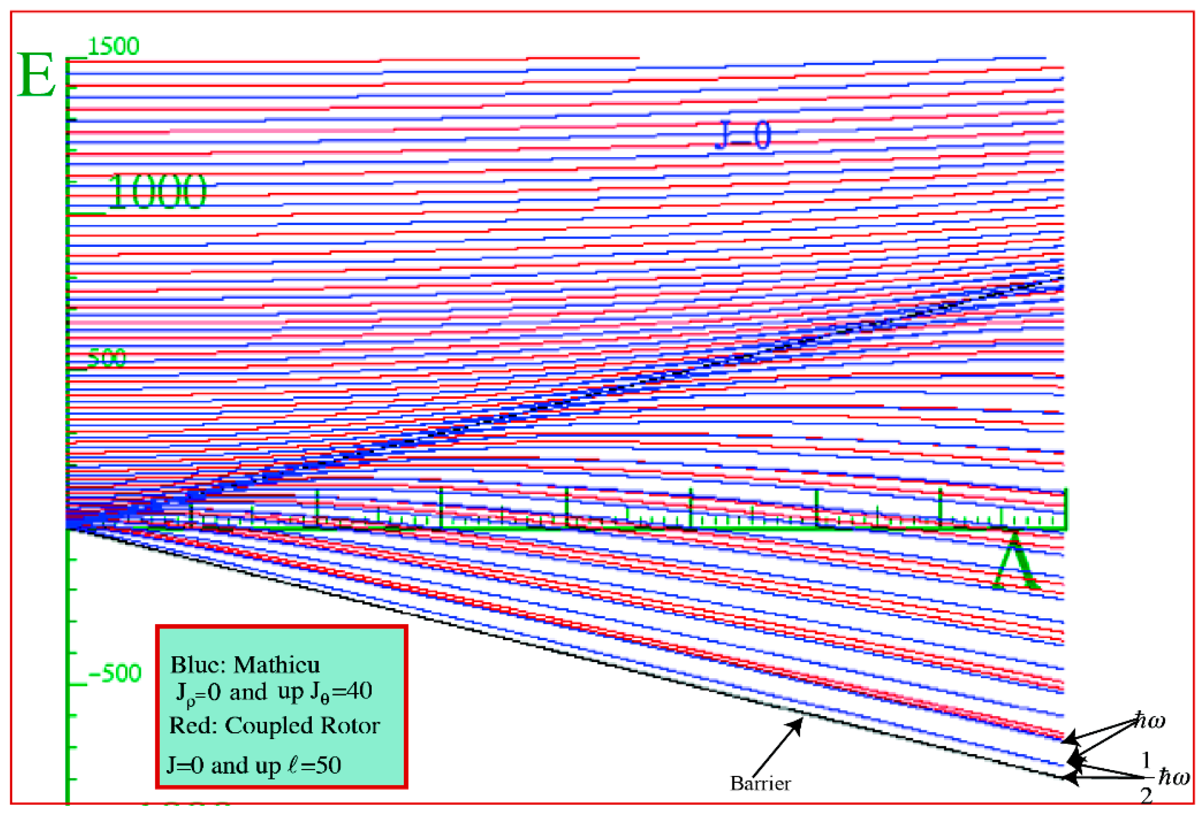
The red curves in (
Figure 7) are those due to the Hamiltonian Equation (20) of two coupled rotors. The blue curves come as a result of solving the Mathieu Equation (21). The black lines in the figure are the top and bottom of the potential barrier. We expect that at
J = 0, our simple model will be present in the three-dimensional system.
Figure 7.
The comparison of the energy behavior above and behavior with the coupling constant between the two rotors model and the super-Mathieu for J = 0 and ℓ = 50.
Figure 7.
The comparison of the energy behavior above and behavior with the coupling constant between the two rotors model and the super-Mathieu for J = 0 and ℓ = 50.
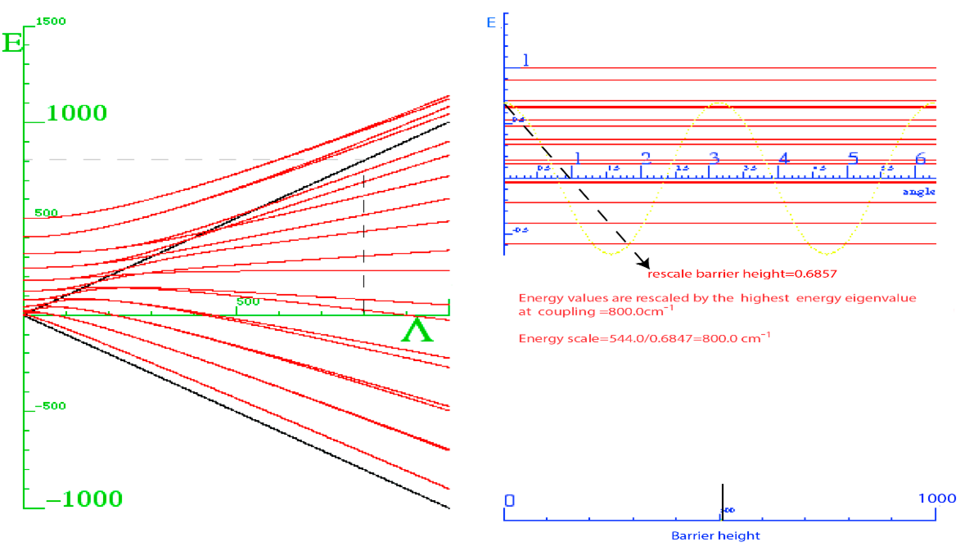
Our strategy is to supper-impose the blue curves that were obtained by solving Equation (21a) onto the red energy spectrum curves, which are the eigenvalue solutions of Equation (18). In the low coupling limit (LWC) we observe that both sets of energy spectrum were quasi-quadratic above the barrier (
Figure 8). This is an indication that our coupled system is loosely correlated or very floppy. While in the high limit (BOA), that is below the barrier, we found that the levels come together to form doublets and exhibit near linear behavior between the relative spacing of these doublets in both the simple and 3D-coupled systems. Our Hamiltonian is a function of angular
ℓ,
R and
J. For the plot shown in
Figure 7,
J = 0,
ℓ = 50 and
R = ⎥
𝐽 −
ℓ⎥. Thus the number of states considered was 51. If we do not include enough states, the red curves would curve away as the barrier is approaching from the left to give a similar behavior as the blue curves above the barrier shown in
Figure 7. At low energy, the doublets squeeze tighter together. This is strong evidence that the rotors are becoming locked together to form a single composite rotor.
Figure 8.
Left: Energy vs. coupling constant for Equation (21) with JΘ = 10 and Bℓ = BR = 2.5 cm−1; Right: Displaying the potential energy curve and energy levels at single coupling constant Λ = 800 cm−1 and barrier height = 540 cm−1.
Figure 8.
Left: Energy vs. coupling constant for Equation (21) with JΘ = 10 and Bℓ = BR = 2.5 cm−1; Right: Displaying the potential energy curve and energy levels at single coupling constant Λ = 800 cm−1 and barrier height = 540 cm−1.
2.2.3. Coupling Behavior of the Simple Rotor Model with the Full 3D Model of Two Coupled Rotor-Systems
We are eluded by the fact that there is not a match for the lower energy of the simple model with that of the coupled system. Oftentimes a shift comes about in matrix equation if the diagonal terms are changing. As a result, we investigated the interaction term of our rotor-coupled system and found that there are terms on the diagonal that are due to the coupling (this behavior is due to the centrifugal distortion). In comparison to the interaction of the Mathieu equation, there are no such terms in the simple model.
Consequently, we now introduce such a term into the Mathieu equation to do just that. When we first wrote down the Hamiltonian for two particles moving on a ring, a term resulted in on-diagonal terms due to the interaction, which was discarded. Putting this term back caused the Mathieu curves to shift too far upwards. Thus we introduced a fractional parameter (b) to control the shift.
When b = 0.125, a more realistic match is reproduced between the Mathieu and the two-coupled rotor system. However as we increase the coupling to value greater than 800 there is a noticeable mismatch between the lowest energy spectra of the blue curves with that of the red curves. This is an indication that the shift was not a result of the absence of the on-diagonal term in the simple model. Yet, another way to understand the shift is to change the inertia constant in our simple model. There seems to be a match in the lines when the inertia is eight times the original. However, this does not seem to be the mechanism for the shift since most of the other lines are off. The explanation for this shift is that simple Mathieu is 1D but the coupled system has a higher degree of freedom.
In the Mathieu model, the first level matches the zero point of a 1D harmonic oscillator, whereas the lowest level for J = 0 in the coupled system corresponds to a 3D oscillator. We will next consider higher Js and observe what happens there.
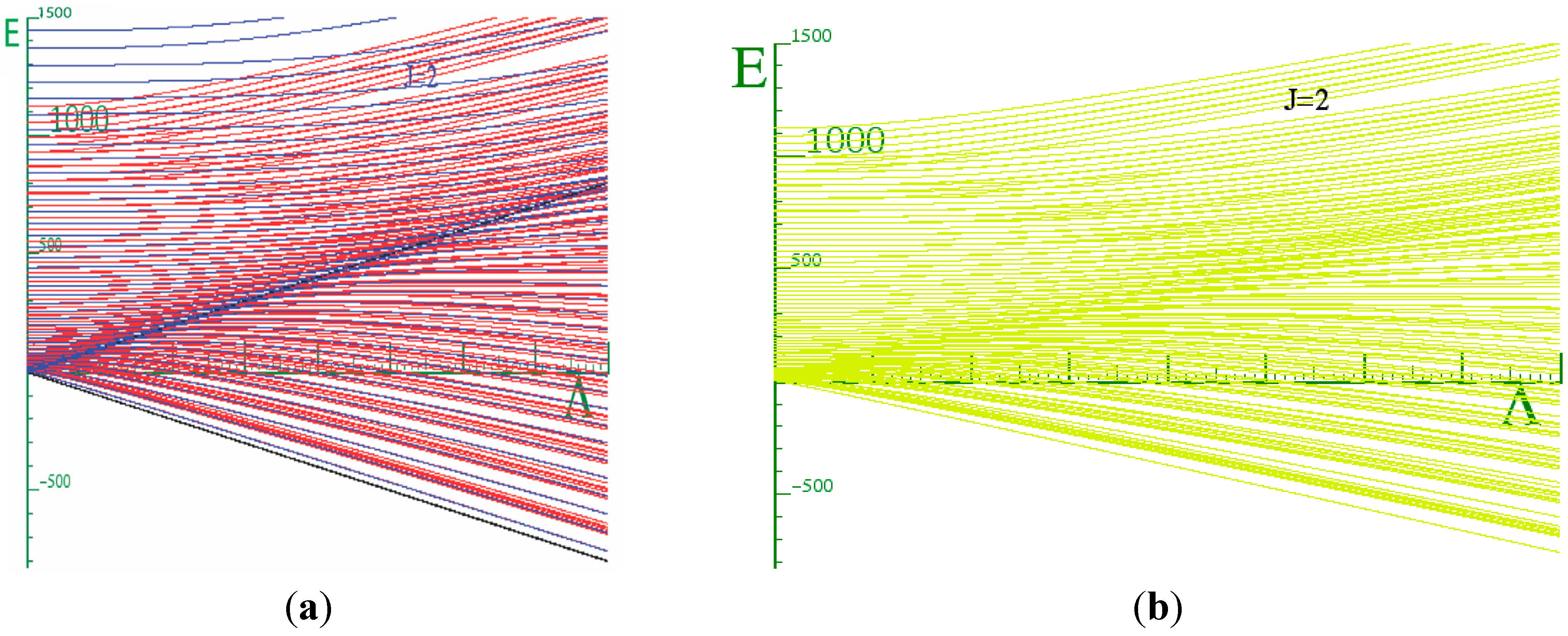
We solved the Hamiltonian for
J = 1, 2, and 3 and found that there is a perfect correspondence between the lowest energy of the Mathieu system and the coupled rotor system (
Figure 9) for
J ≥ 2. There is a strong indication that our system becomes locked as we go to very high coupling constants. We observed a quadratic behavior above the barrier, which is an indication of the degree of floppiness in our system. A linear behavior in the energy was observed as illustrated by (
Figure 8). This corresponds to a system that is extremely correlated or locked. When this happens, the system moves together as one unit while vibrating rapidly.
Figure 9.
(a) Energy Spectrum for the two coupled rotor models super-imposed on the super-Mathieu for J = 2; (b) Energy Spectrum for the two coupled rotor models for J = 2 display alone.
Figure 9.
(a) Energy Spectrum for the two coupled rotor models super-imposed on the super-Mathieu for J = 2; (b) Energy Spectrum for the two coupled rotor models for J = 2 display alone.
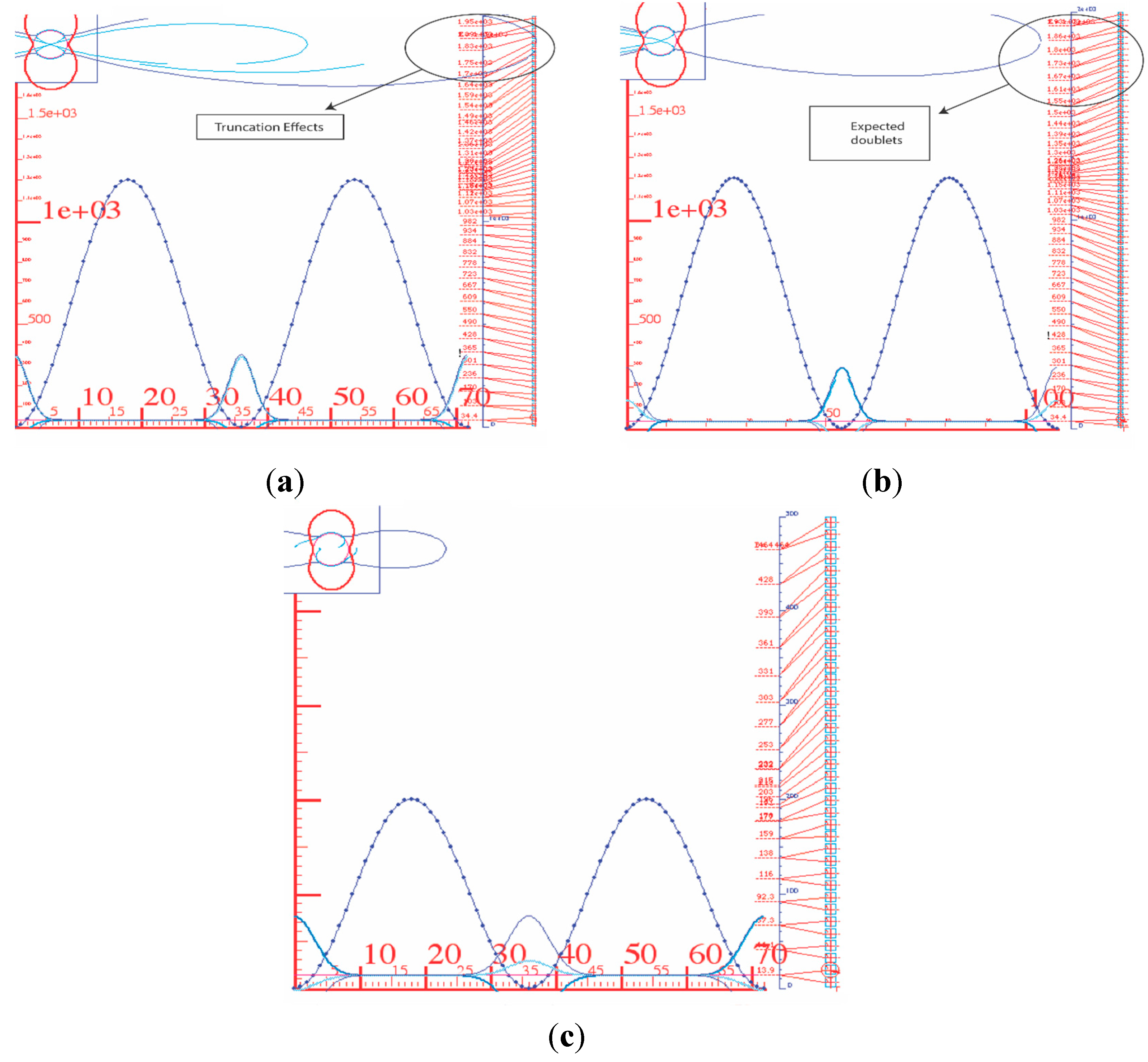
2.3. Truncation Effects in a Coupled Rotor System
In
Figure 5, the lower energy states are doubly degenerated, but they split near the top of the barrier. However, they recombine into different doubly degenerated energy levels as the coupling constant increases. For higher energy states they may fail to recombine as a result of truncation of our matrix. The circled region of
Figure 5 shows splitting that arises from truncation above the barrier. To prevent this anti-fact we must introduce more base states. The energy level diagrams in
Figure 10 illustrate truncation effects, where the top states are splitting apart. With the potential barrier in
Figure 10 being large (that is, comparable with the largest energy level) and
JΘ = 36, only the levels below the barrier height may be trusted since those above the barrier are no longer expected to be quadratic doublets.
Figure 10.
Energy level diagrams. (a) High-energy truncation effects occur for a high barrier (V = 1200 cm−1) and a low truncation value (JΘ = 36); (b) High-energy truncation effects reduced for higher truncation values (JΘ = 54); (c) Effects on truncation effects reduced for (V = 200 cm−1).
Figure 10.
Energy level diagrams. (a) High-energy truncation effects occur for a high barrier (V = 1200 cm−1) and a low truncation value (JΘ = 36); (b) High-energy truncation effects reduced for higher truncation values (JΘ = 54); (c) Effects on truncation effects reduced for (V = 200 cm−1).
Figure 10b, with a higher truncation value (
JΘ = 54), shows the expected quadratic behavior above the barrier. Note that when the top of the barrier is much lower (
JΘ = 36) (
Figure 10c), then we still observe a quadratic spacing above the barrier in spite of low (↓) truncation values. This indicates where the diagonalization may be valid.
The full rotor–rotor diagonalization also shows truncation effects with respect to the cut-off of the ℓ values used in the starting basis. It is important to see how truncated ℓ affects the calculation. To this end we consider another simple model, the particle orbiting a 2D-cosine potential or “a particle orbiting in a peanut”.
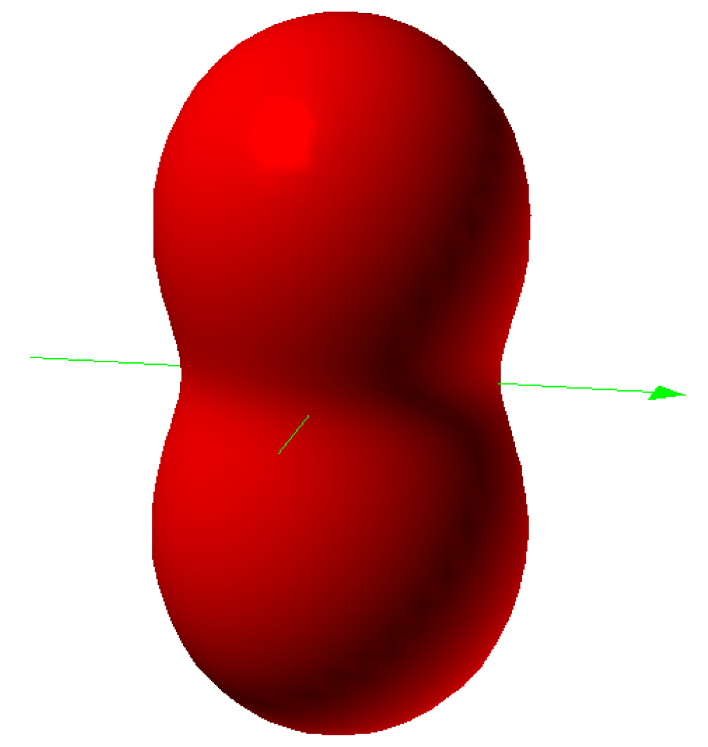
2.4. Orbits in 2D-Cosine Potential (“Particle in a Peanut”)
Let’s consider a particle constrained to move on a peanut-like potential surface shown in (
Figure 11). The Hamiltonian of this model is as follows:
The wavefunction is given by superposition of the spherical harmonics ⎥
ℓm〉 or
![Ijms 15 19662 i029]()
.
where
![Ijms 15 19662 i032]()
are elements of the eigenvectors after the diagonalizing H. The Hamiltonian matrix Equation (25) to be diagonalized is given by:
Figure 11.
Potential surface of a “peanut”.
Figure 11.
Potential surface of a “peanut”.
2.4.1. Probability Distribution Comparison between a Rotor–Rotor Model and a Particle in 2D Cosine Potential
The angular
![Ijms 15 19662 i033]()
state probability is the square of the elements in the eigenvectors as in Equation (26), that is:
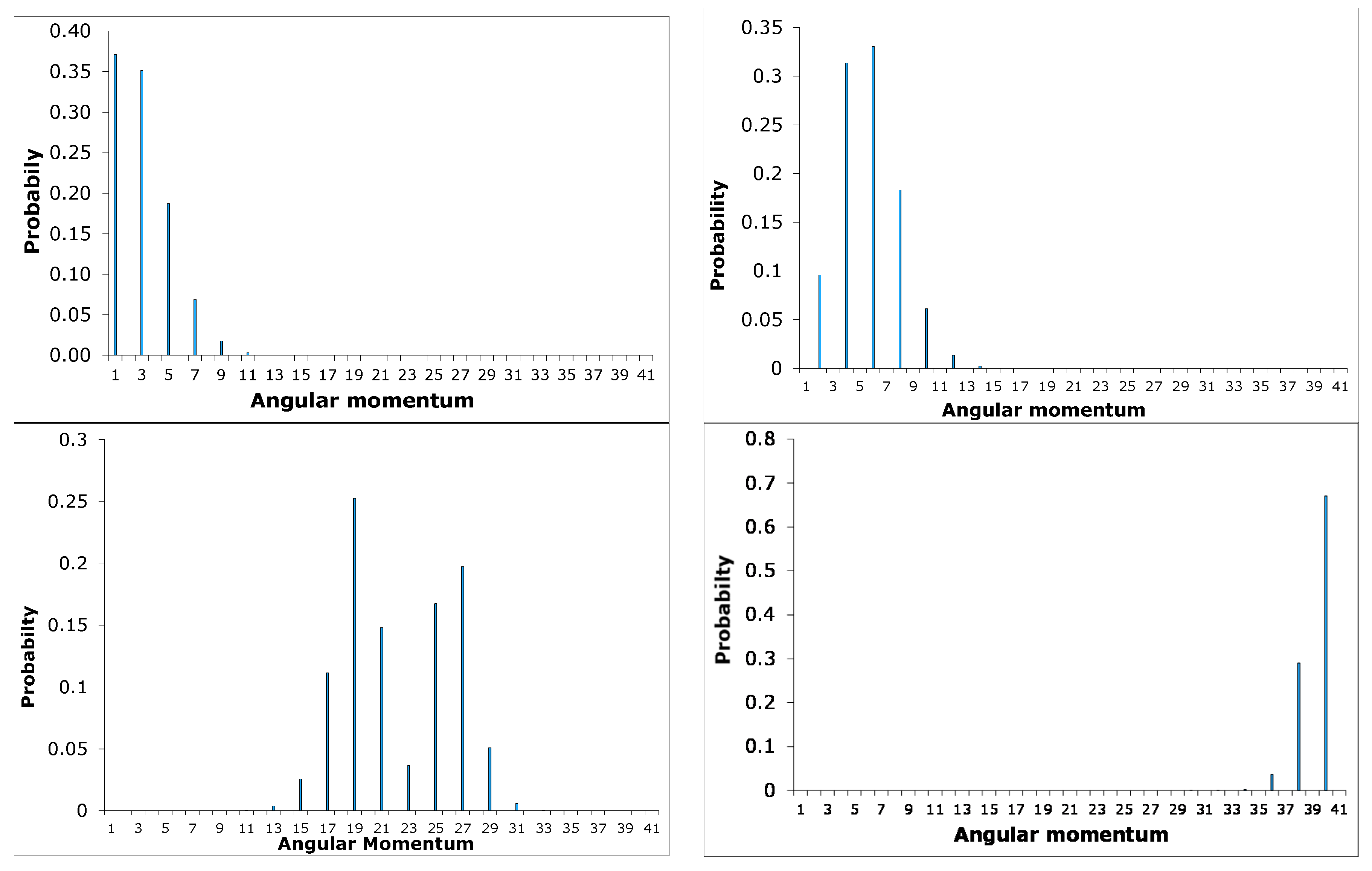
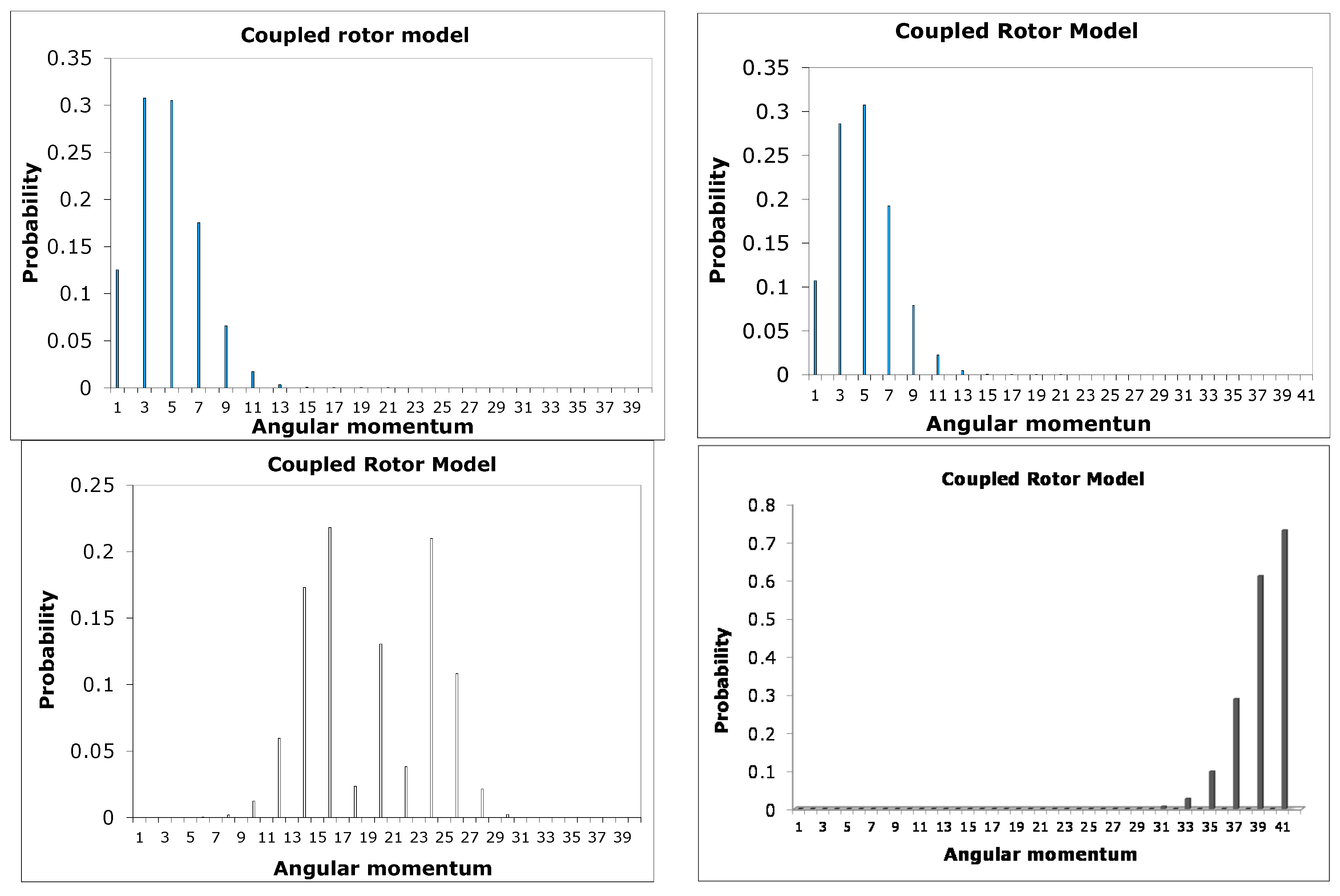
Figure 12 shows a plot of probability
![Ijms 15 19662 i035]() vs. ℓ
vs. ℓ for corresponding
Eℓm and
m-values = 0, 1, 2…
We compare
m = 0 for a single particle constrained to move on the surface of a peanut-like shape with the two coupled rotors for
J = 0. It was observed that there is good correspondence in the behavior of their probability distribution as illustrated in
Figure 12 and
Figure 13. They both start out Poissonian, however, as the angular momentum
ℓ increases their distributions are no longer Poissonian. In other words this behavior in distribution is a non-classical effect.
Figure 12.
Probability distribution at m = 0 for a particle constrained to move on the surface of a “peanut” with ℓ = 0 − 40.
Figure 12.
Probability distribution at m = 0 for a particle constrained to move on the surface of a “peanut” with ℓ = 0 − 40.
Figure 13.
Probability distribution at J = 0 for a particle constrained for two coupled rotors ℓ = 0 − 40.
Figure 13.
Probability distribution at J = 0 for a particle constrained for two coupled rotors ℓ = 0 − 40.
2.4.2. The Determination of Extremely Strongly Coupled Rotors
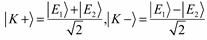
As we move from the LWC basis to the BOA basis by increasing the coupling strength, the two rotors eventually become locked together so that they move as a single system. In the LWC model, the
K quantum number is not good but improves in the BOA region. Our goal here is to find the coupling constant where
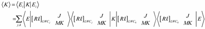
K is good. To do this we must compute the expectation value
K by using the eigenvector of the coupled system as coupling increases. The expectation value of
K is given by:
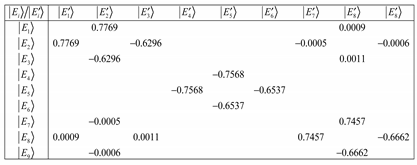
where Equation (27) is a matrix equation that has off-diagonal elements when the coupling is weak. The matrix shown below was computed for
𝐽 = 1,
ℓ = 0.2 and a coupling constant of about 0.08. It is evident that at such weak interactions, we are not in the BOA basis since Equation (28a) shows off-diagonal terms.
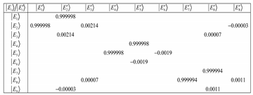
On the other hand, when the coupling constant is about 8000 then Equation (28a) reduces to Equation (28b). Increasing the coupling constant continuously gives Equation (28c). However, we have chosen 𝐽 = 1, ℓ = 0.2 from which at low ℓ values, there will be the issue of truncation error to contend with. The matrix reduces at much lower coupling with a large number of angular momentum ℓ states. This suggests that the more angular momentumstates ℓ states, the more BOA-constricted are the rotors for high coupling values. Because of truncation errors close to the barrier, we are only interested in the K quantum numbers that correspond to the states deep down.
We observed that along the diagonal of Equation (28c) there are two-by-two matrices such as:
which have eigenvalues of +1 or −1. As a result, the eigenvalues are −1 0 1, −1 0 1, and −1 0 1. These are
K quantum numbers for
J = 1. Given that Equation (29) is a B matrix, then the eigenvectors in Equation (30) for the BOA basis are represented by:
Once we know at what coupling constant the
K quantum number is good, then the search for a rotor spectrum can begin. Wilson,
et al. [
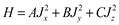
23] were the first to treat the effect of centrifugal distortion in rotational energy level by considering the general rotor Hamiltonian,
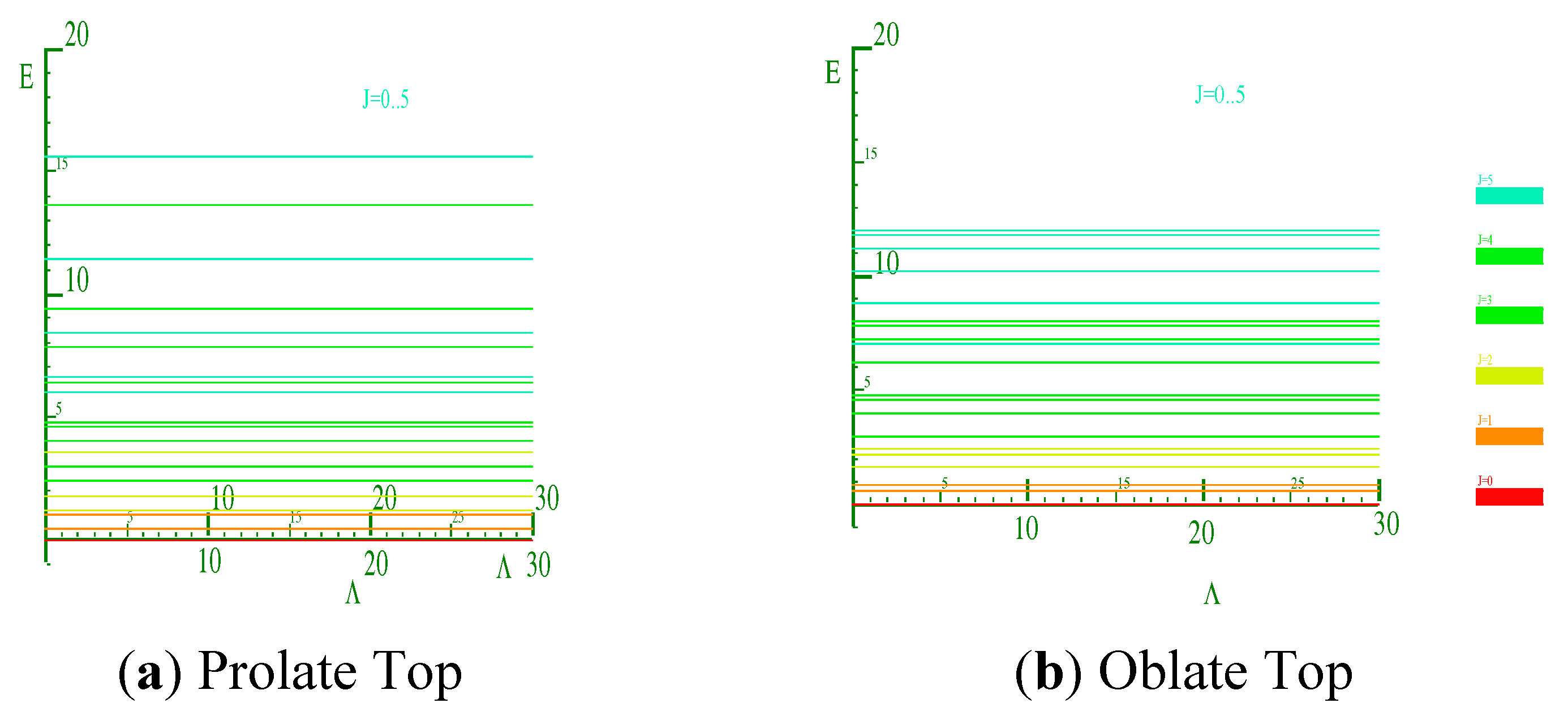
Equation (31) describes three classes of rotor tops: a prolate top if
A = B < C, an oblate top if
B = C > A, and an asymmetric top if
A ≠ B ≠ C. Thus, we illustrate the energy spectrum for a prolate and an oblate tops in
Figure 14 and
Figure 15. The goal here is to compare the spectrum of the composite rotor with that of
Figure 15.
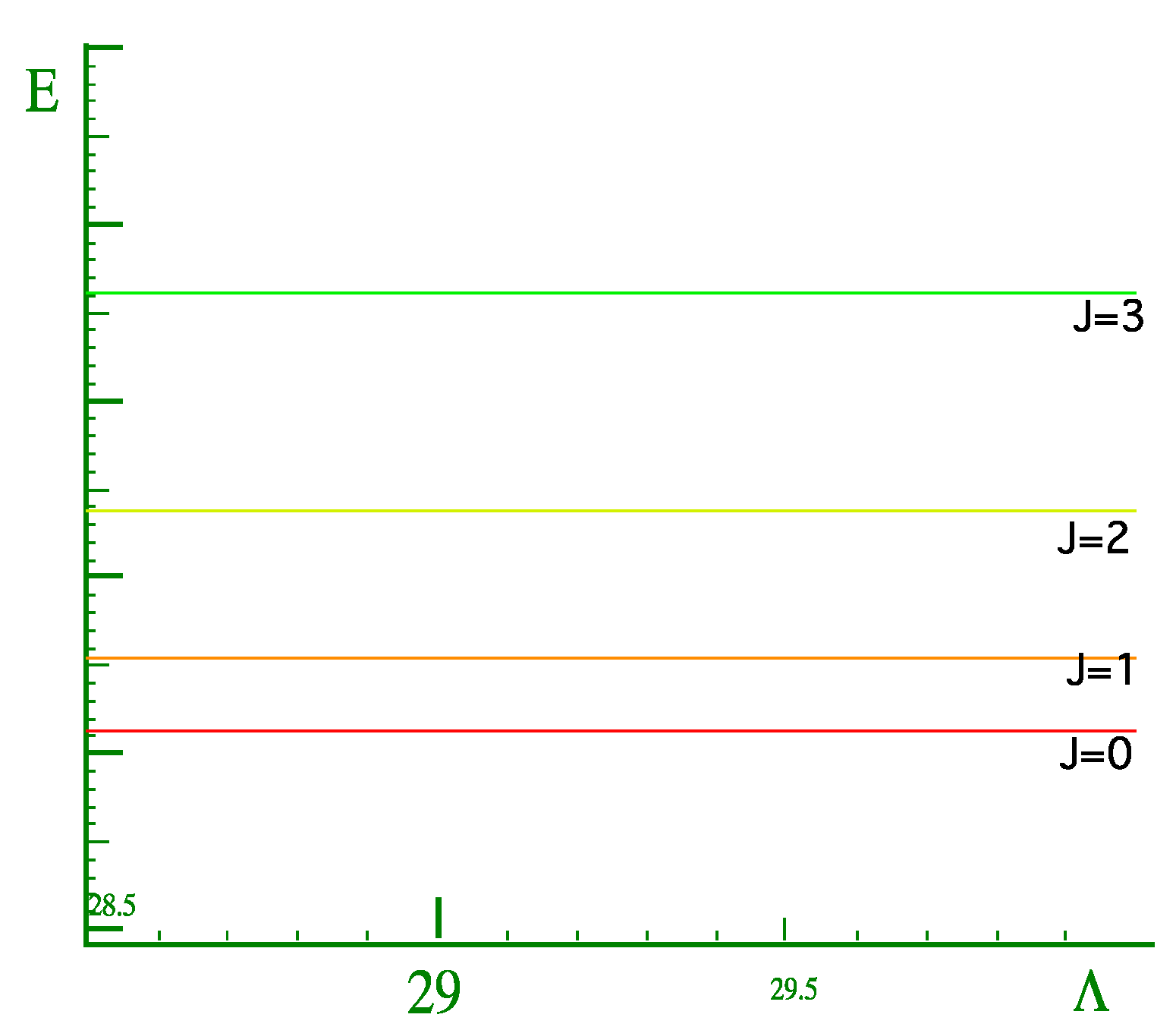
Figure 14.
Quantum rotor levels for J = 0,1,3,….
Figure 14.
Quantum rotor levels for J = 0,1,3,….
Figure 15.
(a) and (b) show the energy spectrum for a prolate and an oblate molecule respectively.
Figure 15.
(a) and (b) show the energy spectrum for a prolate and an oblate molecule respectively.
Recall in
Section 2, that due to truncation effects, only the states below the barrier should be trusted. Therefore, we began the search for a rotor spectrum at lowest energy levels in the energy spectra of the coupled rotor system as shown by (
Figure 16). One should note that a coupling at which the
K quantum numbers become good increases with
J. Recall also that in
Section 2, for the values of
J > 1, we observed that the lowest levels do not have
K = 0. This phenomenon is not clearly understood yet, however, to find a rotor spectrum we must begin the search above these levels or the band of levels where
K = 0 levels may be found.
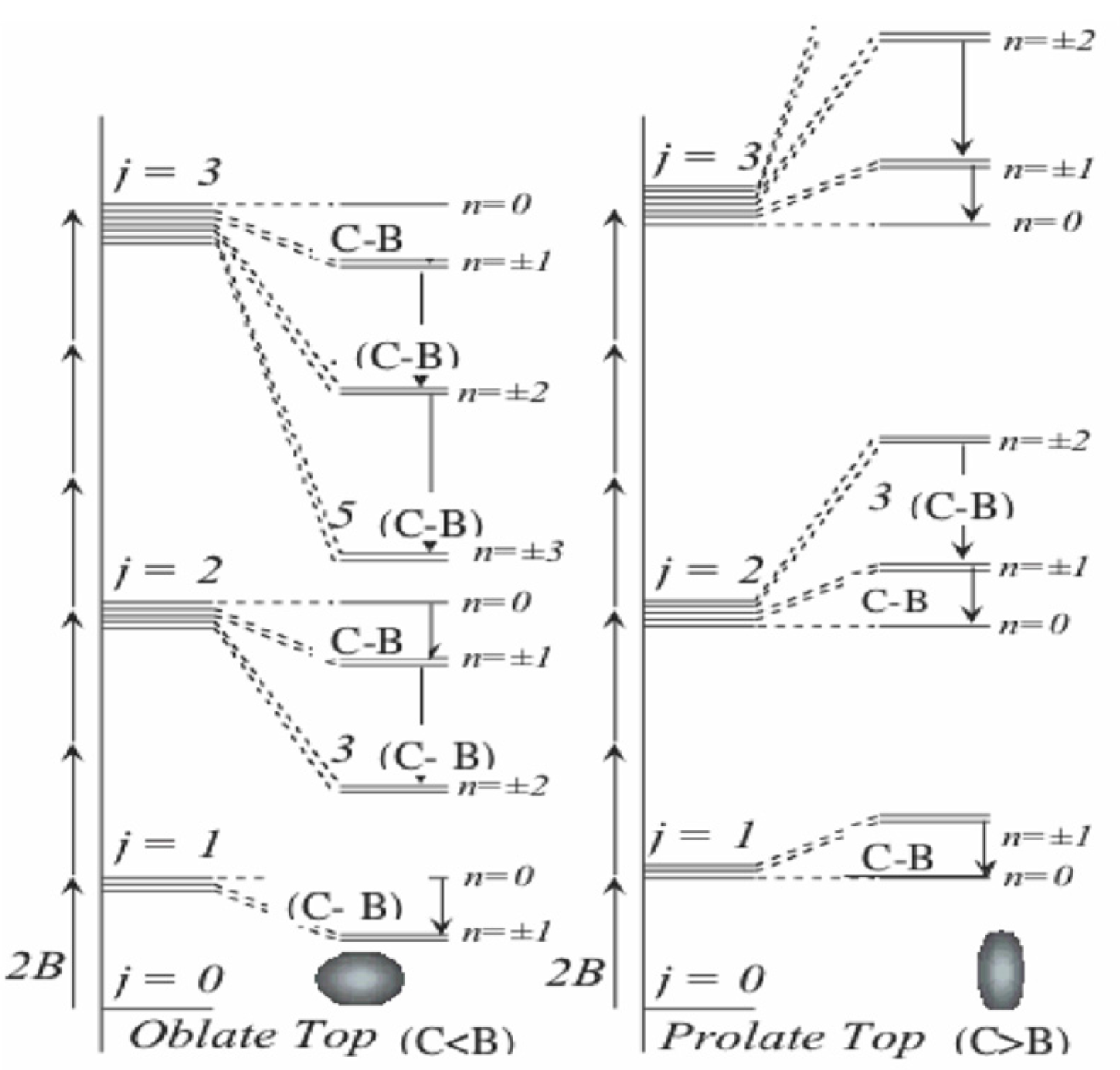
Figure 17 shows the energy spectrum of the rotor molecule for
K = 0 which is obtained from the spectrum of the two coupled rotors as shown in
Figure 16. Although, we are able to find a spectrum for
K = 0, we were unsuccessful in getting a match for
K = 1 or higher values.
K = 0 does not provide us with enough information to decide whether or not we have a prolate spectrum, an oblate spectrum, or something else.
Figure 16.
Energy spectrum, calculated for coupling value of 800,000.0 and J = 0 − 2 and ℓ = 0 − 40. Zoom energy spectrum for the lowest energy band to far right.
Figure 16.
Energy spectrum, calculated for coupling value of 800,000.0 and J = 0 − 2 and ℓ = 0 − 40. Zoom energy spectrum for the lowest energy band to far right.
Figure 17.
Rotor spectrum for a coupled rotor system for K = 0 at the J values shown above.
Figure 17.
Rotor spectrum for a coupled rotor system for K = 0 at the J values shown above.
However, we speculate that our potential does not completely describe the phase space, and as a result the marriage between the two rotors was unsuccessful. Nevertheless, our potential was enough to tell whether or not the system would lock. We did find evidence of locking of the two coupled rotor molecules.


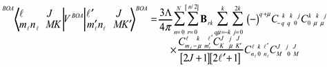
 where z and x are zero. Consequently, the general matrix element of a scalar potential [18,19,20] is given by the following:
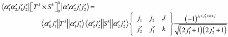

 . This value was rescaled by a factor of 10 on the plot. The plots of Figure 3a,b correspond to the interaction potential in Figure 2 with n = 2 and 3 respectively.


 (one on either side of Θ = π) and one at Θ = π. Therefore, the graph is symmetric at about π. This is a stable point. For n having odd values, the graphs will be symmetric around π. Thus the two diatomic molecules would prefer aligning parallel to each other at Θ = π for N = 3 but have a perpendicular alignment for
  , which corresponds to N = 2.
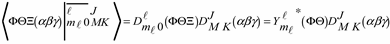


 .
.
 are elements of the eigenvectors after the diagonalizing H. The Hamiltonian matrix Equation (25) to be diagonalized is given by:
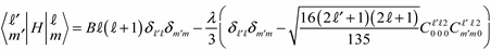

 state probability is the square of the elements in the eigenvectors as in Equation (26), that is:
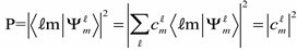
