2D Quantitative Structure-Property Relationship Study of Mycotoxins by Multiple Linear Regression and Support Vector Machine

Abstract
:1. Introduction
2. Results and Discussion
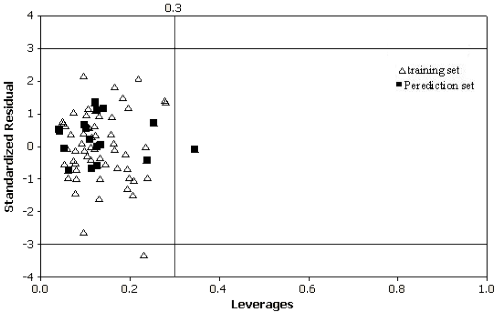
2.1. Definition of the Applicability Domain of the Model
2.2. Interpretation of Descriptors
3. Experimental Section
3.1. Data Set
3.2. Descriptor Generation and Reduction
3.3. Descriptor Selection and Model Building
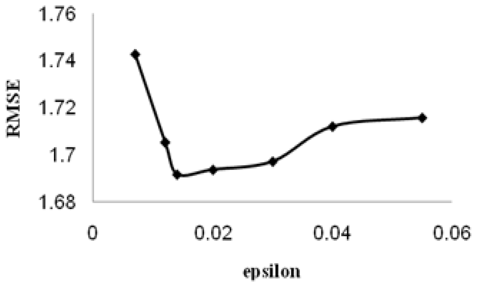
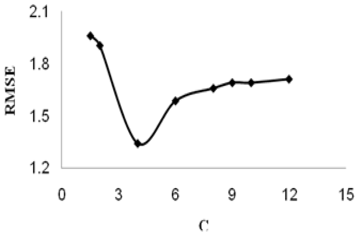
3.4. Theory of SVM
3.5. Validation Test
4. Conclusions
References
- Bennett, JW; Klich, M. Mycotoxins. Clin. Microbiol. Rev 2003, 16, 497–516. [Google Scholar]
- Magan, N; Olsen, M. Mycotoxins in Food Detection and Control; Woodhead Publishing Limited: Cambridge, UK, 2000; p. 7. [Google Scholar]
- Baggiani, C; Giraudi, G; Vanni, A. A molecular imprinted polymer with recognition properties towards the carcinogenic mycotoxin ochratoxin A. Bioseparation 2001, 10, 389–394. [Google Scholar]
- El-Nezami, H; Kankaanpaa, P; Salminen, S; Ahokas, J. Ability of dairy strains of lactic acid bacteria to bind a common food carcinogen, aflatoxin B1. Food Chem. Toxicol 1998, 36, 321–326. [Google Scholar]
- Shephar, GS. Determination of mycotoxins in human foods. Chem. Soc. Rev 2008, 37, 2468–2477. [Google Scholar]
- Frisvad, JC; Thrane, U; Filtenborg, O. Chemical Fungal Taxonomy; Marcel Dekker: New York, NY, USA, 1998; pp. 289–301. [Google Scholar]
- Mantle, PG. Secondary Metabolites of Penicillium and Acremonium; Plenum Press: New York, NY, USA, 1987; pp. 135–151. [Google Scholar]
- Gloer, JB. The chemistry of fungal antagonism and defense. Can. J. Bot 1995, 73, S1265–S1274. [Google Scholar]
- Bull, AT; Ward, AC; Goodfellow, M. Search and discovery strategies for biotechnology: The paradigm shift. Microbiol. Mol. Biol 2002, R64, 573–606. [Google Scholar]
- Bentley, R. Mycophenolic Acid: A One hundred year odyssey from antibiotic to immunosuppressant. Chem. Rev 2000, 100, 3801–3826. [Google Scholar]
- Constant, HL; Beecher, CWW. A method for the dereplication of natural product extracts using electrospray HPLC/MS. Nat. Prod. Lett 1995, 6, 193–196. [Google Scholar]
- Corley, DG; Durley, RC. Strategies for database dereplication of natural products. J. Nat. Prod 1994, 57, 1484–1490. [Google Scholar]
- Nielsen, KF; Smedsgaard, J. Fungal metabolite screening: Database of 474 mycotoxins and fungal metabolites for dereplication by standardised liquid chromatography–UV–mass spectrometry methodology. J. Chromatog. A 2003, 1002, 111–136. [Google Scholar]
- Steinmetz, WE; Rodarte, CB; Lin, A. 3D QSAR study of the toxicity of trichothecene mycotoxins. Eur. J. Med. Chem 2009, 44, 4485–4489. [Google Scholar]
- Song, M; Breneman, CM; Bi, J; Sukumar, N; Bennett, KP; Cramer, S; Tugcu, N. Prediction of protein retention times in anion exchange chromatography systems using support vector regression. J. Chem. Inf. Comput. Sci 2002, 42, 1347–1357. [Google Scholar]
- Yao, XJ; Panaye, A; Doucet, JP; Zhang, RS; Chen, HF; Liu, MC; Hu, ZD; Fan, BT. Comparative study of QSAR/QSPR correlations using support vector machines, radial basis function neural networks, and multiple linear regression. J. Chem. Inf. Comput. Sci 2004, 44, 1257–1266. [Google Scholar]
- Jalali Heravi, M; Konuze, E. Use of quantitative structure property relationships in predicting the Kraft point of anionic surfactants. Int. Electron. J. Mol. Des 2002, 1, 410–417. [Google Scholar]
- Eriksson, L; Jaworska, J; Worth, AP; Cronin, MTD; McDowell, RM; Gramatica, P. Methods for reliability and uncertainty assessment and for applicability evaluations of classification and regression-based QSARs. Environ. Health Perspect 2003, 111, 1361–1375. [Google Scholar]
- Gramatica, P. Principles of QSAR models validation: internal and external. QSAR Comb. Sci 2007, 26, 694–701. [Google Scholar]
- Netzeva, TI; Worth, AP; Aldenberg, T; Benigni, R; Cronin, MTD; Gramatica, P; Jaworska, JS; Kahn, S; Klopman, G; Marchant, CA; Myatt, G; Nikolova-Jeliazkova, N; Patlewicz, GY; Perkins, R; Roberts, DW; Schultz, TW; Stanton, DT; vande Sandt, JJM; Tong, W; Veith, G; Yang, C. Current status of methods for defining the applicability domain of (quantitative) structure–activity relationships. The report and recommendations of ECVAM Workshop 52. Altern. Lab. Anim 2005, 33, 155–173. [Google Scholar]
- Roberts, DW. Application of octanol/water partition coefficients in surfactant science: A quantitative structure-property relationship for micellization of anionic surfactants. Langmuir 2002, 18, 345–352. [Google Scholar]
- Leo, AJ. Calculating log Poct from structures. Chem. Rev 1993, 93, 1281–1306. [Google Scholar]
- Katritzky, AR; Lobanov, VS; Karelson, M. QSPR: The correlation and quantitative prediction of chemical and physical properties from structure. Chem. Soc. Rev 1995, 24, 279–287. [Google Scholar]
- Khan, MS; Khan, ZH. Molecular modeling for generation of structural and molecular electronic descriptors for QSAR using quantum mechanical semiemprical and ab initio methods. Gen. Inf 2003, 14, 486–487. [Google Scholar]
- Ghasemi, J; Abdolmaleki, A; Asadpour, S; Shiri, F. Prediction of solubility of nonionic solutes in anionic micelle (SDS) using a QSPR model. QSAR Comb. Sci 2008, 27, 338–346. [Google Scholar]
- Todeschini, R; Consonni, V; Mannhold, R; Kubinyi, H; Timmerman, H. Handbook of Molecular Descriptors; Wiley-VCH in Weinheim: New York, NY, USA, 2000; pp. 324–345. [Google Scholar]
- Melagraki, G; Afantitis, A. A novel QSPR model for predicting θ (lower critical solution temperature) in polymer solutions using molecular descriptors. J. Mol. Model 2007, 13, 55–64. [Google Scholar]
- Afantitis, A; Melagraki, G; Sarimveis, H; Koutentis, PA; Markopoulos, J; Igglessi-Markopoulou, O. A novel QSAR model for predicting induction of apoptosis by 4-aryl-4H-chromens. Bioorg. Med. Chem 2006, 14, 6686–6694. [Google Scholar]
- Altomare, C; Cellamare, S; Carotti, A; Barreca, ML; Chimirri, A; Monforte, AM; Gasparrini, F; Villani, C; Cirilli, M; Mazza, F. Substituent effects on the enantioselective retention of anti-HIV 5-aryl-Δ2-1,2,4-oxadiazolines on R, R-DACH-DNB chiral stationary phase. Chirality 1996, 8, 556–566. [Google Scholar]
- Altomare, C; Carotti, A; Cellamare, S; Fanelli, F; Gaspar-rini, F; Villani, C; Carrupt, PA; Testa, B. Enantiomeric resolution of sulfoxides on a DACH-DNB chiral stationary phase: A quantitative structure-enantioselective retention relationship (QSERR) study. Chirality 1993, 5, 527–537. [Google Scholar]
- Holland, JH. Genetic algorithms. Sci. Am 1992, 267, 66–72. [Google Scholar]
- Ghasemi, J; Saaidpour, S; Brown, SD. QSPR study for estimation of acidity constants of some aromatic acids derivatives using multiple linear regression (MLR) analysis. J. Mol. Struct 2007, 805, 27–32. [Google Scholar]
- Vapnik, V. The Nature of Statistical Learning Theory; Springer: New York, NY, USA, 1995; pp. 217–231. [Google Scholar]
- Burges, CJC. A tutorial on support vector machines for pattern recognition. Data Min. Knowl. Disc 1998, 2, 1–47. [Google Scholar]
- Vapnik, V. Estimation of Dependences Based on Empirical Data; Springer: Berlin, Germany, 1982; pp. 137–145. [Google Scholar]
- Vapnik, V; Golowich, S; Smola, A. Support vector method for function approximation, regression estimation, and signal processing. In Neural InformationProcessing Systems; MIT Press: Cambridge, MA, USA, 1997; Volume 9, pp. 281–287. [Google Scholar]
- Image Speech and Intelligent Systems Research Group. Applying SVM Toolbox; University of Southampton: Southampton, UK. Available at: http://www.isis.ecs.soton.ac.uk/isystems/kernel/svm.zip (accessed on 16 August 2010).
- Golbraikh, A; Tropsha, A. Beware of q2. J. Mol. Graph. Model 2002, 20, 269–276. [Google Scholar]
- Roy, PP; Roy, K. On some aspects of variable selection for partial least squares regression models. QSAR Comb. Sci 2008, 27, 302–313. [Google Scholar]
- Shapiro, S; Guggenheim, B. Inhibition of oral bacteria by phenolic compounds. Part 1 QSAR analysis using molecular connectivity. Quant. Struct. Act. Relat 1998, 17, 327–337. [Google Scholar]


| Descriptor | Coefficient | Mean effect | VIFe |
|---|---|---|---|
| C logPa | 2.6951(±0.2248) | 5 | 1.006 |
| ElcEb | −0.0002(±0.0001) | 8 | 1.246 |
| DPLLc | −1.091(±0.2981) | −3.875 | 1.556 |
| LUMOd | −1.6922(±0.5521) | 0.594 | 1.287 |
| Constant | 3.1912(±1.7569) | _ | _ |
| tR | C logP | ElcE | DPLL | LUMO | |
|---|---|---|---|---|---|
| tR | 1 | ||||
| C logP | 0.821263 | 1 | |||
| ElcE | −0.21234 | 0.05977 | 1 | ||
| DPLL | −0.07144 | 0.004813 | −0.32903 | 1 | |
| LUMO | −0.12041 | −0.05044 | 0.000773 | −0.45025 | 1 |
| No. | Exp. ( tR) | MLR model | SVM model | ||
|---|---|---|---|---|---|
| Pred. (tR) | RE (%) | Pred. (tR) | RE (%) | ||
| 21 | 5.1 | 4.97 | 2.55 | 5.03 | 1.37 |
| 4 | 6.6 | 6.91 | −4.7 | 7.99 | −21.06 |
| 23 | 7.4 | 7.03 | 5 | 8.35 | −12.84 |
| 41 | 8.59 | 8.88 | −3.38 | 10.08 | −17.35 |
| 3 | 10.33 | 9.44 | 8.62 | 10.25 | 0.77 |
| 38 | 10.51 | 11.43 | −8.75 | 12 | −14.18 |
| 24 | 11.28 | 12.03 | −6.65 | 12.37 | −9.66 |
| 27 | 13.69 | 11.51 | 15.92 | 11.74 | 14.24 |
| 34 | 14.15 | 11.48 | 18.87 | 12.53 | 11.45 |
| 13 | 15.03 | 14.52 | 3.39 | 15.18 | −1 |
| 25 | 15.56 | 14.61 | 6.11 | 14.79 | 4.95 |
| 37 | 17 | 14.29 | 15.94 | 15.08 | 11.29 |
| 11 | 18.02 | 15.7 | 12.87 | 16.37 | 9.16 |
| 46 | 18.6 | 18.91 | −1.67 | 19.39 | −4.25 |
| 65 | 20 | 22.66 | −13.3 | 22.11 | −10.55 |
| 29 | 21.12 | 22.61 | −7.05 | 20.43 | 3.27 |
| 55 | 21.6 | 20.74 | 3.98 | 19.84 | 8.15 |
| Parameters | MLR | SVM |
|---|---|---|
| RMSEP | 1.504 | 1.341 |
| REPa (%) | 10.902 | 9.719 |
| SEPb | 1.551 | 1.382 |
| q2 | 0.915 | 0.932 |
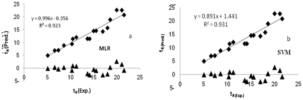
| R2 | 0.923 | 0.931 |
| (R2-R02)/R2 | 0.001 | 0.0118 |
| (R2-R′02)/R2 | 0.0108 | 0.0011 |
| rm2 | 0.894 | 0.833 |
| k | 0.996 | 0.891 |
| k′ | 0.926 | 1.045 |
| NDSc | 4 | 4 |
| NO. | Compound | tR(min) | NO. | Compound | tR(min) |
|---|---|---|---|---|---|
| Aflatoxins and their precursors | |||||
| 1 | Aflatoxicol I | 12.45 | 9 | Austocystin A | 21.57 |
| 2 | Aflatoxin B1 | 11.50 | 10 | Averufin | 25.65 |
| 3 | Aflatoxin B2 | 10.33 | 11 | 5-Methoxysterigmatocystin | 18.02 |
| 4 | Aflatoxin B2 α | 6.60 | 12 | Dihydroxysterigmatocystin | 17.70 |
| 5 | Aflatoxin G1 | 10.16 | 13 | Methoxysterigmatocystin | 15.03 |
| 6 | Aflatoxin G2 | 8.97 | 14 | Sterigmatocystin | 18.91 |
| 7 | Aflatoxin G2α | 5.00 | 15 | Norsolorinic acid | 31.08 |
| 8 | Aflatoxin M1 | 7.21 | 16 | Parasiticol | 10.73 |
| Trichothecenes | |||||
| 17 | Nivalenol | 1.27 | 27 | HT-2 Toxin | 13.69 |
| 18 | Fusarenone X | 2.35 | 28 | T-2 Toxin | 17.06 |
| 19 | Deoxynivalenol | 1.54 | 29 | Acetyl-T-2 toxin | 21.12 |
| 20 | 3-Acetyldeoxynivalenol | 5.21 | 30 | Trichodermin | 16.13 |
| 21 | 15-O-Acetyl-4- deoxynivalenol | 5.10 | 31 | Trichodermol | 9.69 |
| 22 | Scirpentriol | 1.82 | 32 | 7-α-Hydroxytrichodermol | 2.59 |
| 23 | 15-Acetoxyscirpenol | 7.40 | 33 | Verrucarol | 2.89 |
| 24 | Diacetoxyscirpenol | 11.28 | 34 | 4,15-Diacetylverrucarol | 14.15 |
| 25 | 3α-Acetyldiacetoxyscirpenol | 15.56 | 35 | Trichothecin | 16.29 |
| 26 | Neosolaniol | 3.19 | 36 | Trichothecolone | 3.63 |
| 37 | Trichoverrol A | 10.16 | |||
| Roquefortines, ergot amines and related alkaloids | |||||
| 38 | Agroclavine-I | 17.00 | 51 | Ergotamin | 19.60 |
| 39 | Auranthine | 10.51 | 52 | Fumigaclavine C | 21.40 |
| 40 | Aurantiamine | 10.49 | 53 | Marcfortine A | 19.59 |
| 41 | Aurantioclavine | 14.30 | 54 | Marcfortine B | 17.39 |
| 42 | Chanoclavine-I | 8.59 | 55 | Meleagrin | 18.90 |
| 43 | Costaclavine | 17.00 | 56 | Oxalin | 21.60 |
| 44 | Cyclopenin | 11.60 | 57 | Pyroclavine | 14.81 |
| 45 | Cyclopenol | 6.20 | 58 | Roquefortine C | 20.50 |
| 46 | Cyclopeptin | 12.05 | 59 | Roquefortine D | 6.09 |
| 47 | Dihydroergotamin | 18.60 | 60 | Rugulovasine A and B | 8.43 |
| 48 | Elymoclavine | 5.34 | 61 | Secoclavine | 20.40 |
| 49 | Epoxyagroclavine-I | 10.00 | 62 | α-Ergocryptin | 19.20 |
| 50 | Ergocristine | 25.10 | |||
| Ochratoxins | |||||
| 63 | Ochratoxin α | 5.60 | 66 | Ochratoxin B-ethyl ester | 19.41 |
| 64 | Ochratoxin A-methyl ester | 22.49 | 67 | Ochratoxin α-methyl ester | 16.16 |
| 65 | Ochratoxin B-methyl ester | 20.00 | |||
| Cross-Validation | Random subset |
|---|---|
| Number of subsets | 4 |
| Population size | 64 |
| Mutation rate | 0.005 |
| Window width | 2 |
| Initial term% | 20% |
| Maximum generation | 100 |
| Convergence (%) | 50 |
| Cross-over | Double |
© 2010 by the authors; licensee Molecular Diversity Preservation International, Basel, Switzerland. This article is an open-access article distributed under the terms and conditions of the Creative Commons Attribution license (http://creativecommons.org/licenses/by/3.0/).
Share and Cite
Khosrokhavar, R.; Ghasemi, J.B.; Shiri, F. 2D Quantitative Structure-Property Relationship Study of Mycotoxins by Multiple Linear Regression and Support Vector Machine. Int. J. Mol. Sci. 2010, 11, 3052-3068. https://doi.org/10.3390/ijms11093052
Khosrokhavar R, Ghasemi JB, Shiri F. 2D Quantitative Structure-Property Relationship Study of Mycotoxins by Multiple Linear Regression and Support Vector Machine. International Journal of Molecular Sciences. 2010; 11(9):3052-3068. https://doi.org/10.3390/ijms11093052
Chicago/Turabian StyleKhosrokhavar, Roya, Jahan Bakhsh Ghasemi, and Fereshteh Shiri. 2010. "2D Quantitative Structure-Property Relationship Study of Mycotoxins by Multiple Linear Regression and Support Vector Machine" International Journal of Molecular Sciences 11, no. 9: 3052-3068. https://doi.org/10.3390/ijms11093052
APA StyleKhosrokhavar, R., Ghasemi, J. B., & Shiri, F. (2010). 2D Quantitative Structure-Property Relationship Study of Mycotoxins by Multiple Linear Regression and Support Vector Machine. International Journal of Molecular Sciences, 11(9), 3052-3068. https://doi.org/10.3390/ijms11093052