
Solvatochromic and Computational Study of Three Benzo-[f]-Quinolinium Methylids with Photoinduced Charge Transfer


Abstract

1. Introduction
2. Results and Discussion
2.1. Experimental Solvatochromism of I1, I2 and I3
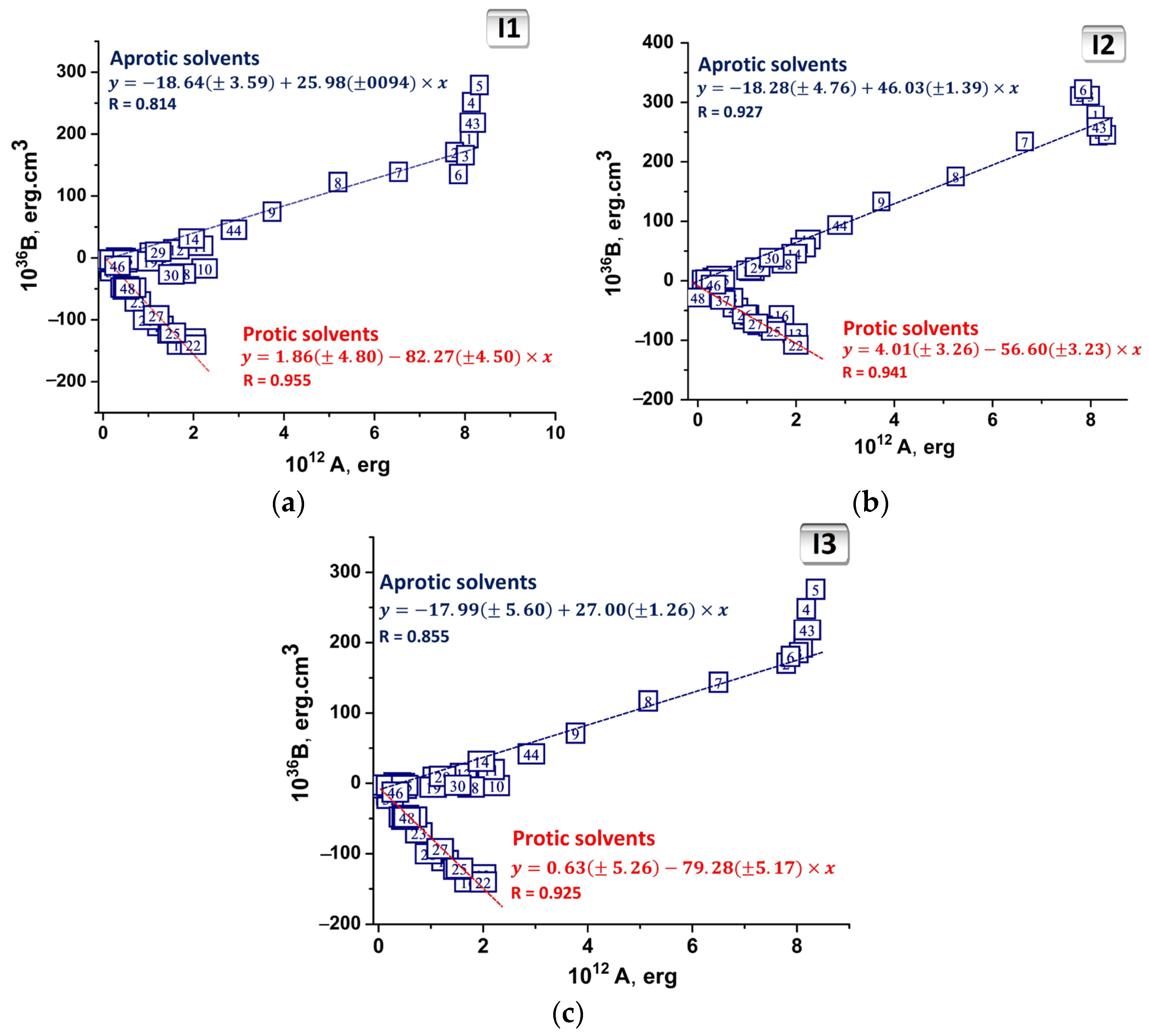
2.2. Abe’s Model of the Liquid
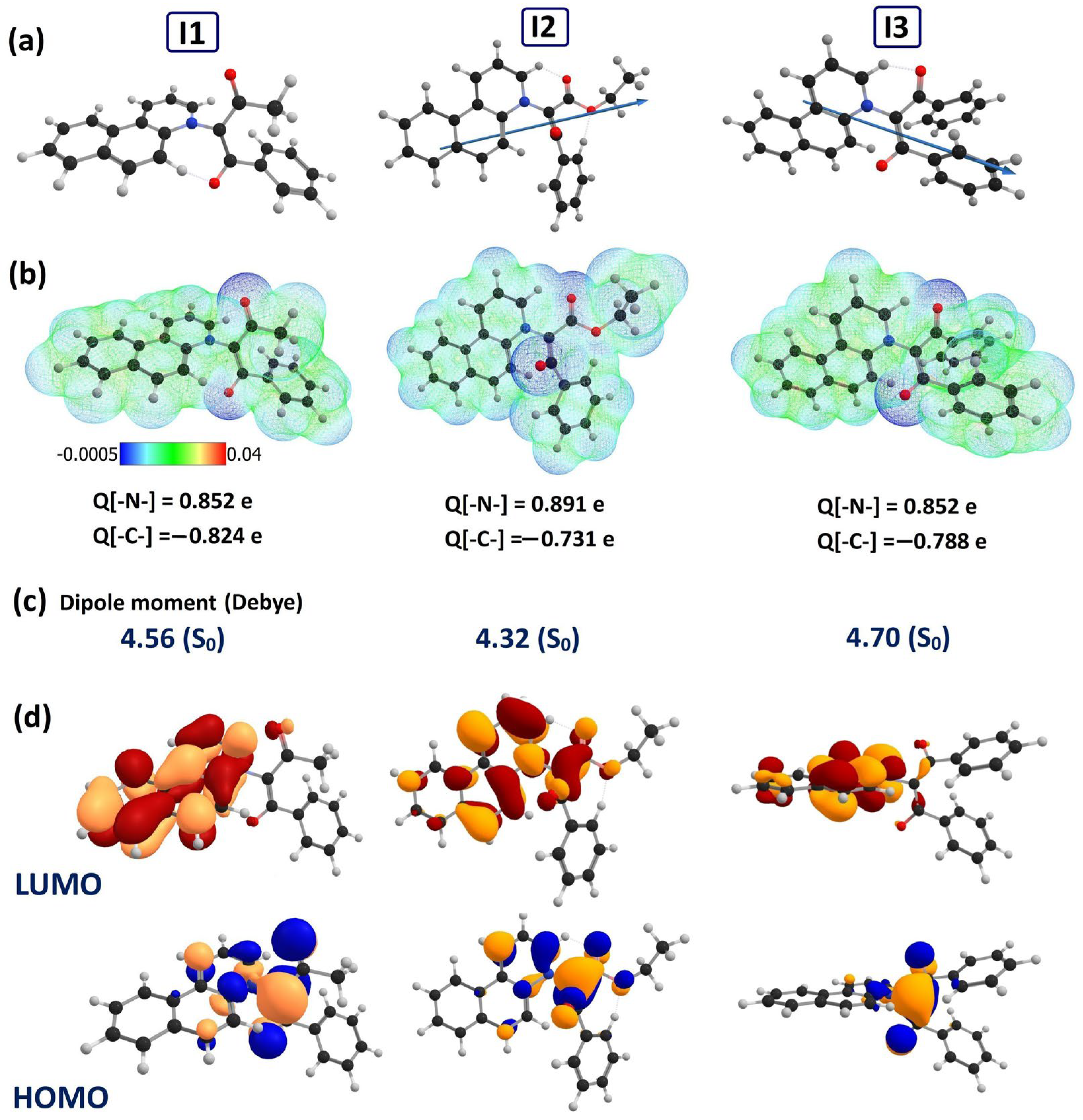
2.3. Quantum Chemical Investigations of I1, I2 and I3
3. Materials and Methods
4. Conclusions
Supplementary Materials
Author Contributions
Funding
Institutional Review Board Statement
Informed Consent Statement
Data Availability Statement
Conflicts of Interest
References
- Ledade, P.V.; Lambat, T.L.; Gunjate, J.K.; Chopra, P.K.P.G.; Bhute, A.V.; Lanjewar, M.R.; Kadu, P.M.; Dongre, U.J.; Mahmood, S.H. Nitrogen-containing fused heterocycles: Organic synthesis and applications as potential anticancer agents. Curr. Org. Chem. 2023, 27, 206–222. [Google Scholar] [CrossRef]
- Zbancioc, G.; Mangalagiu, I.I.; Moldoveanu, C. The effective synthesis of new benzoquinoline derivatives as small molecules with anticancer activity. Pharmaceuticals 2024, 17, 52. [Google Scholar] [CrossRef] [PubMed]
- Antoci, V.; Oniciuc, L.; Amariucai–Mantu, D.; Moldoveanu, C.; Mangalagiu, V.; Amarandei, A.M.; Lungu, C.N.; Dunca, S.; Mangalagiu, I.I.; Zbancioc, G. Benzoquinoline derivatives: A straightforward and efficient route to antibacterial and antifungal agents. Pharmaceuticals 2021, 14, 335. [Google Scholar] [CrossRef] [PubMed]
- Boateng, C.A.; Zhu, X.Y.; Jacob, M.R.; Khan, S.I.; Walker, L.A.; Ablordeppey, S.Y. Optimization of 3 (phenylthio)quinolinium compounds against opportunistic fungal pathogens. Eur. J. Med. Chem. 2011, 46, 1789–1797. [Google Scholar] [CrossRef]
- Boateng, C.A.; Eyunni, S.V.K.; Zhu, X.Y.; Etukala, J.R.; Bricker, B.A.; Ashfaq, M.K.; Jacob, M.R.; Khan, S.I.; Walker, L.A.; Ablordeppey, S.Y. Benzothieno [3,2-b]Quinolinium and 3(phenylthio)quinolinium compounds: Synthesis and evaluation against opportunistic fungal pathogens. Bioorg. Med. Chem. 2011, 19, 458–470. [Google Scholar] [CrossRef]
- Yamamoto, K.; Torigoe, K.; Kuriyama, M.; Demizu, Y.; Onomura, O. (3+2) Cycloaddition of Heteroaromatic N-Ylides with Sulfenes. Org. Lett. 2024, 26, 798–803. [Google Scholar] [CrossRef]
- Liu, F.-T.; Zhai, S.-M.; Gao, D.-F.; Yang, S.-H.; Zhao, B.-X.; Lin, Z.-M. A Highly Sensitive Ratiometric Fluorescent Probe for Detecting HSO3−/SO32− and Viscosity Change Based on FRET/TICT Mechanism. Anal. Chim. Acta 2024, 1305, 342588. [Google Scholar] [CrossRef]
- Wang, M.-Q.; Zhang, Y.; Zeng, X.-Y.; Yang, H.; Yang, C.; Fu, R.-Y.; Li, H.-J. A Benzo(f)Quinolinium fused chromophore-based fluorescent probe for selective detection of c-Myc G-quadruplex DNA with a red emission and a large Stockes shift. Dye. Pigment. 2019, 168, 334–340. [Google Scholar] [CrossRef]
- Zugravescu, I.; Petrovanu, M. N-Ylid Chemistry; McGraw Hill: New York, NY, USA; Academic Press: London, UK, 1976. [Google Scholar]
- Dorohoi, D.; Partenie, H. The Spectroscopy of the cycloimmonium ylides. J. Mol. Struct. 1993, 293, 129–132. [Google Scholar] [CrossRef]
- Teran, N.B.; He, G.S.; Baev, A.; Shi, Y.; Swihart, M.T.; Prasad, P.N.; Marks, T.J.; Reynolds, J.R. Twisted Thiophene-Based Chromophores with Enhanced Intramolecular Charge Transfer for Cooperative Amplification of Third-Order Optical Nonlinearity. J. Am. Chem. Soc. 2016, 138, 6975–6984. [Google Scholar] [CrossRef]
- Zelichenok, A.; Burtman, V.; Zenou, N.; Yitzchaik, S.; Di Bella, S.; Meshulam, G.; Kotler, Z. Quinolinium-Derived Acentric Crystals for Second-Order NLO Applications with Transparency in the Blue. J. Phys. Chem. B 1999, 103, 8702–8705. [Google Scholar] [CrossRef]
- Onsager, L. Electric Moments of Molecules in Liquids. J. Am. Chem. Soc. 1936, 58, 1486–1493. [Google Scholar] [CrossRef]
- Wang, X.; Dao, R.; Yao, J.; Peng, D.; Li, H. Modification of the Onsager Reaction Field and Its Application on Spectral Parameters. ChemPhysChem 2017, 18, 763–771. [Google Scholar] [CrossRef]
- Abe, T. Theory of solvent effects on molecular electronic spectra. Frequency shifts. Bull. Chem. Soc. Jpn. 1965, 38, 1314–1318. [Google Scholar] [CrossRef]
- Abe, T. The Dipole Moments and Polarizabilities in the Excited States of Four Benzene Derivatives from Spectral Solvent Shifts. Bull. Chem. Soc. Jpn. 1967, 40, 1571–1574. [Google Scholar] [CrossRef]
- McRae, E.G. Theory of Solvent Effects on Molecular Electronic Spectra. Frequency Shifts. J. Phys. Chem. 1957, 61, 562–572. [Google Scholar] [CrossRef]
- Kawski, A. On the estimation of excited-state dipole moments from solvatochromic shifts of absorption and fluorescence spectra. Z. Naturforsch. 2002, 57, 255–262. [Google Scholar] [CrossRef]
- Kamlet, M.J.; Abboud, J.I.; Taft, R.W. The solvatochromic comparison method 6. The π* scale of solvent polarities. J. Am. Chem. Soc. 1977, 99, 6027–6038. [Google Scholar] [CrossRef]
- Kamlet, M.J.; Abboud, J.L.M.; Abraham, M.H.; Taft, R.W. Linear solvation energy relationships. 23. A comprehensive collection of the solvatochromic parameters π*, α, and β, and some methods for simplifying the generalized solvatochromic equation. J. Org. Chem. 1983, 48, 2877–2887. [Google Scholar] [CrossRef]
- Kamlet, M.J.; Abboud, J.I.; Taft, R.W. An examination of linear solvation energy relationships. Prog. Phys. Org. Chem. 1981, 13, 485–630. [Google Scholar] [CrossRef]
- Reichardt, C. Solvents and Solvent effects in Organic Chemistry, 3rd ed.; Wiley-VCH: Weinheim, Germany, 2003. [Google Scholar]
- Catalán, J.; Hopf, H. Empirical Treatment of the Inductive and Dispersive Components of Solute−Solvent Interactions: The Solvent Polarizability (SP) Scale. Eur. J. Org. Chem. 2004, 2004, 4694–4702. [Google Scholar] [CrossRef]
- Van Do, N.; Rucinschi, E.; Druta, I.; Zugravescu, I. Recherches sur les benzo(f)quinoléinium-ylures. I. Synthèse de benzo(f)quinoléinium-ylures. Bull. Inst. Pol. Iasi 1977, 23, 53–58. [Google Scholar]
- Dorohoi, D.O.; Partenie, D.H.; Calugaru, A.C. Specific and Universal Interactions in Benzo-[f]-Quinolinium Acetyl-Benzoyl Methylid (BQABM) Solutions; Excited State Dipole Moment of BQABM. Spectrochim. Acta A 2019, 213, 184–191. [Google Scholar] [CrossRef] [PubMed]
- Hilliard, I.J.; Foulk, D.S.; Gold, H.S.; Rechisteiner, C.F. Effects of solute-solvent interactions on electronic spectra-a predictive analysis. Anal. Chim. Acta 1981, 133, 319–327. [Google Scholar] [CrossRef]
- Gulseven Sidir, Y.; Sidir, I.; Beker, H.; Tasal, E. UV spectral changes for some azo-compounds in the presence of different solvents. J. Mol. Liquids 2011, 162, 148–154. [Google Scholar] [CrossRef]
- Sidir, I.; Gulseven Sidir, Y.; Demiray, F.; Berker, H. Estimation of ground and excited states dipole moments of α-hydroxy-phenyl hydrazone derivatives. J. Mol. Liquids 2014, 197, 386–394. [Google Scholar] [CrossRef]
- Morosanu, A.C.; Gritco-Todirascu, A.; Creanga, D.E.; Dorohoi, D.O. Computational and solvatochromic study of pyridinium-acetyl-benzoyl-methylid (PABM). Spectrochim. Acta A 2018, 189, 307–315. [Google Scholar] [CrossRef]
- Dorohoi, D.O.; Dimitriu, D.G.; Dimitriu, M.; Closca, V. Specific interactions in N-ylid solutions, studied by nuclear magnetic resonance and electronic absorption spectropscopy. J. Mol. Struct. 2013, 1044, 79–86. [Google Scholar] [CrossRef]
- Dorohoi, D.O.; Gosav, S.; Morosanu, A.C.; Dimitriu, D.G.; Apreotesei, G.; Gosav, S. Molecular descriptors-spectral property relations for characterization molecular interactions in binary and ternary solutions. Symmetry 2023, 15, 2075. [Google Scholar] [CrossRef]
- Dorohoi, D.O.; Partenie, D.H.; Chiran, L.M.; Anton, C. About the electronic absorption spectra (EAS) and electronic diffusive spectra (EDS) of some pyridazinium ylids. J. Chim. Phys. Phys.-Chim. Biol. 1994, 91, 419–431. [Google Scholar] [CrossRef]
- Avădănei, M.I.; Griţco-Todiraşcu, A.; Dorohoi, D.O. Negative solvatochromism of the intramolecular charge transfer band in two structurally related pyridazinium Ylids. Symmetry 2024, 16, 1531. [Google Scholar] [CrossRef]
- Avadanei, M.I.; Dorohoi, D.O. Comparative Study of Two Spectral Methods for Estimating the Excited State Dipole Moment of Non-Fluorescent Molecules. Molecules 2024, 29, 3358. [Google Scholar] [CrossRef]
- Frisch, M.J.; Trucks, G.W.; Schlegel, H.B.; Scuseria, G.E.; Robb, M.A.; Cheeseman, J.R.; Scalmani, G.; Barone, V.; Mennucci, B.; Petersson, G.A.; et al. Gaussian 09, Revision, A.02; Gaussian, Inc.: Wallingford, CT, USA, 2009. [Google Scholar]
- Pant, D.; Sitha, S. Roles of bridges on electronic, linear and nonlinear optical properties: A computational study on zwitterions with N-methyl pyridinium and p-dicyanomethanide phenylene. Comput. Theor. Chem. 2023, 1229, 114308. [Google Scholar] [CrossRef]
- Liu, Z.; Lu, T.; Chen, Q. An sp-hybridized all-carboatomic ring, cyclo [18] carbon: Electronic structure, electronic spectrum, and optical nonlinearity. Carbon 2020, 165, 461–467. [Google Scholar] [CrossRef]


| No. | ε | f(ε) | f(n) | π* | β | α | ν (nm) I1 | ν (nm) I2 | ν (nm) I3 |
|---|---|---|---|---|---|---|---|---|---|
| 1 | n-Heptane | 0.227 | 0.24 | −0.08 | 0 | 0 | 476 | 477 | 500 |
| 2 | n-Hexane | 0.241 | 0.229 | −0.04 | 0 | 0 | 476 | 477 | 496 |
| 3 | Dioxane | 0.286 | 0.251 | 0.55 | 0.37 | 0 | 473 | 475 | 486 |
| 4 | Carbon tetrachloride | 0.292 | 0.274 | 0.28 | 0.1 | 0 | 472 | 476 | 497 |
| 5 | Benzene | 0.299 | 0.295 | 0.59 | 0.1 | 0 | 454 | 485 | 488 |
| 6 | p-Xylene | 0.299 | 0.291 | 0.13 | 0 | 452 | 487 | 490 | |
| 7 | 1,3,5-Trimethylbenzene | 0.302 | 0.293 | 0.41 | 0.13 | 0 | 453 | 488 | 487 |
| 8 | o-Xylene | 0.302 | 0.292 | 0.41 | 0.11 | 0 | 459 | 491 | 495 |
| 9 | Toluene | 0.348 | 0.297 | 0.54 | 0.11 | 0 | 459 | 494 | 492 |
| 10 | Propanoic acid | 0.434 | 0.239 | 0.45 | 1.12 | 411 | 414 | 406 | |
| 11 | Trichloroethylene | 0.448 | 0.282 | 0.48 | 0.05 | 0 | 463 | 481 | 485 |
| 12 | Methoxybenzene | 0.524 | 0.302 | 0.73 | 0.32 | 0 | 456 | 472 | 478 |
| 13 | 1,2-Dibromoethane | 0.538 | 0.313 | 0 | 0 | 458 | 476 | 478 | |
| 14 | Chloroform | 0.552 | 0.267 | 0.69 | 0.1 | 0.2 | 465 | 476 | 465 |
| 15 | Butyl acetate | 0.577 | 0.24 | 0.46 | 0.45 | 0 | 462 | 474 | 463 |
| 16 | 3-Methylbutyl acetate | 0.589 | 0.241 | 0.71 | 0.07 | 0 | 465 | 468 | 466 |
| 17 | Chlorobenzene | 0.605 | 0.307 | 0.71 | 0.07 | 0 | 453 | 467 | 482 |
| 18 | Ethyl acetate | 0.625 | 0.228 | 0.55 | 0.45 | 0 | 454 | 467 | 479 |
| 19 | Methyl acetate | 0.655 | 0.221 | 0.6 | 0.42 | 0 | 459 | 465 | 469 |
| 20 | Dichloromethane | 0.727 | 0.256 | 0.82 | 0.1 | 0.2 | 459 | 458 | 474 |
| 21 | Octan-1-ol | 0.745 | 0.258 | 0.4 | 0.81 | 0.77 | 438 | 426 | 435 |
| 22 | 1,2-Dichloroethane | 0.752 | 0.264 | 0.81 | 0.1 | 0 | 459 | 465 | 472 |
| 23 | Pyridine | 0.79 | 0.299 | 0.87 | 0.64 | 0 | 455 | 457 | 468 |
| 24 | Hexan-1-ol | 0.839 | 0.252 | 0.04 | 0.84 | 0.8 | 436 | 437 | 428 |
| 25 | Phenylmethanol | 0.804 | 0.311 | 0.98 | 0.52 | 0.6 | 435 | 416 | 416 |
| 26 | Cyclohexanol | 0.824 | 0.276 | 0.45 | 0.84 | 0.66 | 435 | 417 | 422 |
| 27 | Pentan-1-ol | 0.826 | 0.241 | 0.4 | 0.86 | 0.84 | 432 | 415 | 418 |
| 28 | Butan-1-ol | 0.833 | 0.242 | 0.47 | 0.84 | 0.84 | 425 | 416 | 418 |
| 29 | 1-Phenylethanone | 0.833 | 0.312 | 0.9 | 0.49 | 0.04 | 455 | 462 | 466 |
| 30 | Butan-2-one | 0.85 | 0.232 | 0.48 | 0.06 | 452 | 454 | 462 | |
| 31 | Cyclohexanone | 0.85 | 0.269 | 0.76 | 0.53 | 0 | 454 | 454 | 466 |
| 32 | 2-Methylpropan-1-ol | 0.852 | 0.239 | 0.4 | 0.84 | 0.69 | 426 | 414 | 422 |
| 33 | Propan-2-ol | 0.852 | 0.234 | 0.48 | 0.84 | 0.76 | 423 | 420 | 417 |
| 34 | Propan-1-ol | 0.866 | 0.239 | 0.52 | 0.9 | 0.84 | 425 | 412 | 411. |
| 35 | Acetone | 0.868 | 0.222 | 0.62 | 0.48 | 0.08 | 450 | 456 | 466 |
| 36 | Propane-1,2-diol | 0.882 | 0.259 | 0.8 | 0.58 | 421 | 414 | 414 | |
| 37 | 4-Hydroxy-4-methylpentan-2-one | 0.883 | 0.253 | 0.65 | 0.55 | 0 | 425 | 416 | 420 |
| 38 | Pentane-2,4-dione | 0.892 | 0.269 | 0.6 | 0 | 451 | 453 | 462 | |
| 39 | Ethanol | 0.895 | 0.221 | 0.86 | 0.75 | 0.86 | 424 | 414 | 413 |
| 40 | Methanol | 0.909 | 0.203 | 0.6 | 0.66 | 0.98 | 416 | 413 | 407 |
| 41 | Propane-1,3-diol | 0.915 | 0.263 | 0.85 | 0.77 | 411 | 414 | 406 | |
| 42 | Acetonitrile | 0.921 | 0.219 | 0.75 | 0.4 | 0.19 | 449 | 451 | 450 |
| 43 | Dimethylformamide | 0.924 | 0.258 | 0.88 | 0.69 | 0 | 444 | 451 | 454 |
| 44 | Ethane-1,2-diol | 0.93 | 0.259 | 0.9 | 0.52 | 0.9 | 410 | 409 | 402 |
| 45 | Dimethylsulfoxide | 0.946 | 0.281 | 1 | 0.76 | 0 | 446 | 449 | 450 |
| 46 | Propane-1,2,3-triol | 0.948 | 0.28 | 1.14 | 0.7 | 408 | 405 | 400 | |
| 47 | Water | 0.964 | 0.206 | 1.09 | 0.47 | 1.17 | 405 | 404 | 402 |
| 48 | Formamide | 0.973 | 0.271 | 0.97 | 0.48 | 0.71 | 420 | 415 | 416 |
| Compound | Pπ* (%) | Pα (%) | Pβ (%) |
|---|---|---|---|
| I1 | 28.17 | 52.80 | 19.02 |
| I2 | 18.39 | 46.83 | 34.76 |
| I3 | 22.03 | 48.04 | 29.92 |
| Parameter | I1 | I2 | I3 |
|---|---|---|---|
| (eV) | −5.21 | −5.21 | −5.23 |
| (eV) | −2.36 | −2.53 | −2.39 |
| 4.56 | 4.319 | 4.708 | |
| 41.077 | 45.12 | 34.50 | |
| A (Å2) | 306.67 | 328.43 | 360.88 |
| V (Å3) | 313.87 | 339.65 | 368.71 |
| r3 (Å3) | 28.94 | 29.86 | 28.79 |
| I1 | ||
| I2 | ||
| I3 | ||
| φ (degree) | ) | φ (degree) | ) | ||
|---|---|---|---|---|---|
| 0 | 3.88 | 38.16 | 76 | 18.18 | −0.61 |
| 20 | 4.13 | 37.92 | 77 | 20.09 | −9.59 |
| 40 | 5.08 | 36.84 | 78 | 22.58 | −22.65 |
| 60 | 7.91 | 32.32 | 79 | 26.07 | −43.54 |
| 75 | 16.65 | 6.01 | 80 | 31.81 | −84.31 |
| φ (degree) | ) | φ (degree) | ) | ||
|---|---|---|---|---|---|
| 0 | 3.07 | 43.75 | 78.8 | 18.93 | 0.87 |
| 20 | 3.27 | 43.60 | 78.9 | 19.19 | −0.33 |
| 40 | 3.94 | 43.00 | 79 | 19.45 | −1.60 |
| 60 | 6.24 | 40.12 | 80 | 21.99 | −14.54 |
| 75 | 12.92 | 24.41 | 81. | 28.67 | −56.09 |
| 78.5 | 1.72 | 18.21 | 81.5 | 35.46 | −109.5 |
| φ (degree) | ) | φ (degree) | ) | ||
|---|---|---|---|---|---|
| 0 | 3.81 | 32.99 | 77 | ||
| 20 | 4.06 | 32.75 | 78 | 21.87 | −23.85 |
| 40 | 4.99 | 31.71 | 79 | 25.10 | −42.42 |
| 60 | 7.76 | 27.38 | 80 | 30.13 | −76.44 |
| 75 | 16.25 | 2.41 | 81 | 43.24 | −194.29 |
| BfQ | Solvent | Equation | ||
|---|---|---|---|---|
| I1 | Aprotic | )A | 1.47 | 25.98 |
| Protic | )A | 4.76 | −82.27 | |
| I2 | Aprotic | )A | 4.02 | 46.03 |
| Protic | )A | 6.59 | −56.60 | |
| I3 | Aprotic | )A | 4.92 | 27.00 |
| Protic | )A | 4.77 | −79.28 |
| BfQ | Solvent | Dipole Moment, (D) | Dipole Moment, (D) | Mulliken Charges (e) | Mulliken Charges (e) |
|---|---|---|---|---|---|
| Planar | Non-Planar | Planar | Non-Planar | ||
| I1 | Gas | 4.256 | 4.742 | Q[-N-] = 0.852 Q[-C-] = −0.824 | Q[-N-] = 0.861 Q[-C-] = −0.769 |
| CHX | 4.470 | 4.76 | Q[-N-] = 0.898 Q[-C-] = −0.781 | Q[-N-] = 0.833 Q[-C-] = −0.809 | |
| Water | 6.055 | 5.968 | Q[-N-] = 0.880 Q[-C-] = −0.800 | Q[-N-] = 0.793 Q[-C-] = −0.770 | |
| I2 | Vacuum | 4.209 | 5.050 | Q[-N-] = 0.901 Q[-C-] = −0.731 | Q[-N-] = 0.865 Q[-C-] = −0.786 |
| CHx | 4.32 | 6.094 | Q[-N-] = 0.892 Q[-C-] = −0.718 | Q[-N-] = 0.837 Q[-C-] = −0.789 | |
| Water | 6.283 | 7.189 | Q[-N-] = 0.865 Q[-C-] = −0.762 | Q[-N-] = 0.796 Q[-C-] = −0.776 | |
| I3 | Vacuum | 4.526 | Q[-N-] = 0.852 Q[-C-] = −0.788 | ||
| CHx | 4.825 | Q[-N-] = 0.842 Q[-C-] = −0.812 | |||
| Water | 6.494 | Q[-N-] = 0.821 Q[-C-] = −0.775 | |||
| In Vacuum | Planar Conformation | Non-Planar Conformation |
|---|---|---|
| Conformation | 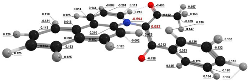 Q[-N-] = − 0.594 Q[-N-] = − 0.594Q[-C-] = 0.082 μe = 2.27 D |  Q[-N-] = − 0.565 Q[-N-] = − 0.565Q[-C-] = 0.048 μe = 3.53 D |
| Hole–electron distribution | 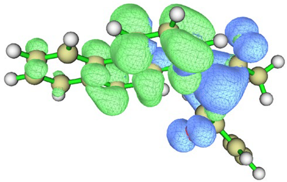 | 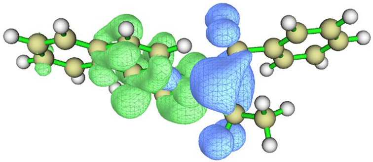 |
| Charge density difference |  | 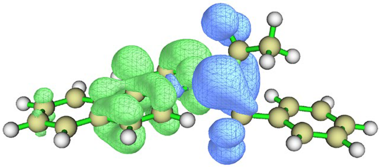 |
| In CHX | Planar Conformation | Non-Planar Conformation |
| Conformation |  Q[-N-] = −0.576 Q[-N-] = −0.576Q[-C-] = 0.101 μe = 2.77 D | 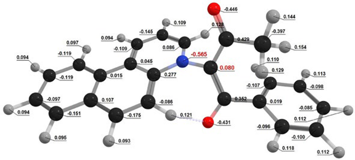 Q[-N-] = −0.565 Q[-N-] = −0.565Q[-C-] = 0.080 μe = 4.87 D |
| Hole–electron distribution | 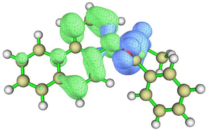 | 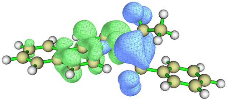 |
| Charge density difference | 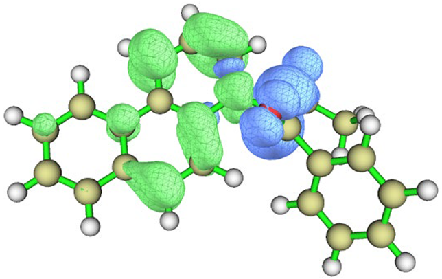 |  |
| In Water | Planar Conformation | Non-Planar Conformation |
| Conformation | 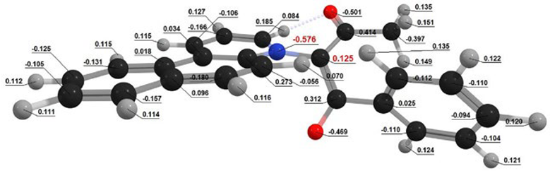 Q[-N-] = −0.576 Q[-N-] = −0.576Q[-C-] = 0.125 μe = 4.15 D | 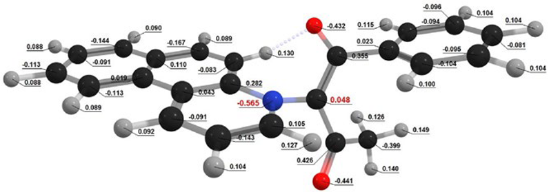 Q[-N-] = −0.565 Q[-N-] = −0.565Q[-C-] = 0.048 μe = 6.09 D |
| Hole–electron distribution |  | 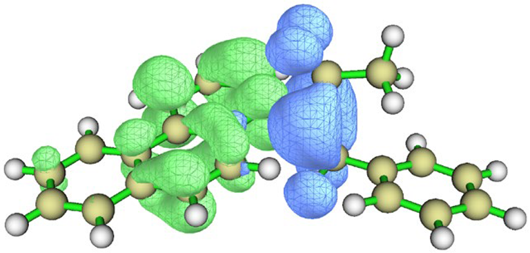 |
| Charge density difference | 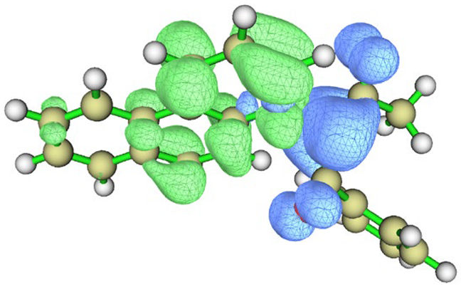 |  |
| BfQ | Solvent | Hole–Electron Distribution | Charge Density Difference |
|---|---|---|---|
| I2 | vacuum | 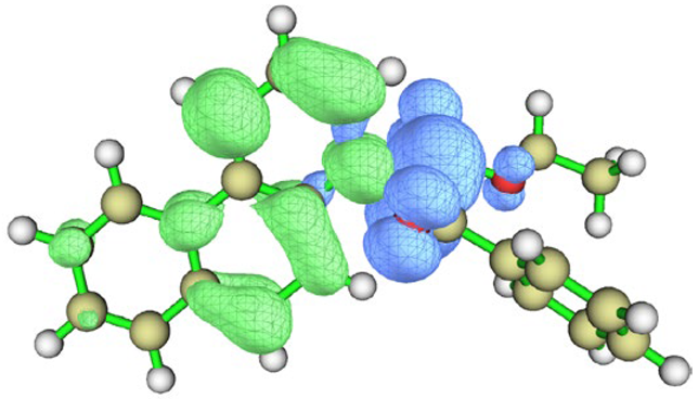 |  |
| cyclohexane | 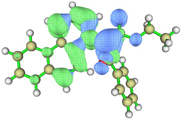 | 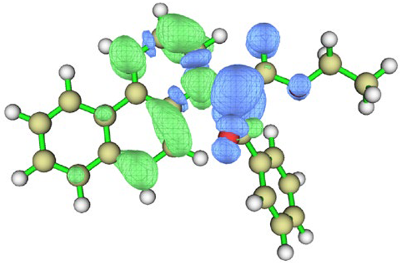 | |
| water |  | 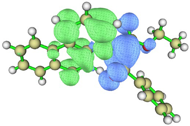 | |
| I3 | vacuum | 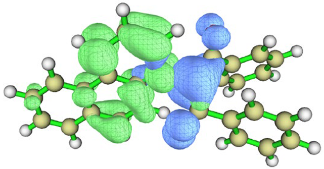 | 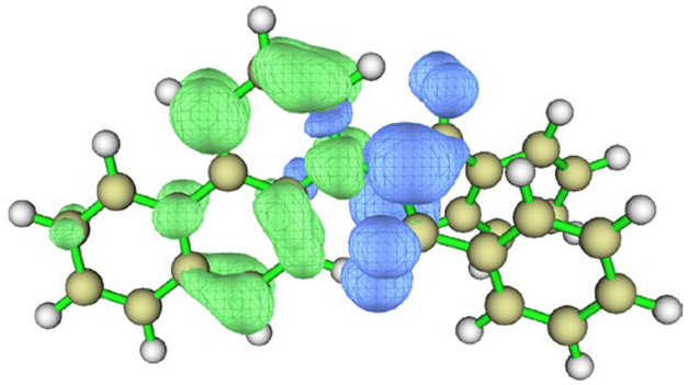 |
| cyclohexane |  | 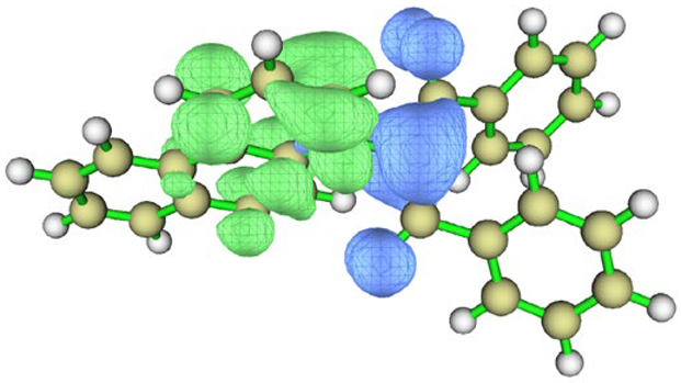 | |
| water |  | 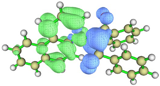 |
Disclaimer/Publisher’s Note: The statements, opinions and data contained in all publications are solely those of the individual author(s) and contributor(s) and not of MDPI and/or the editor(s). MDPI and/or the editor(s) disclaim responsibility for any injury to people or property resulting from any ideas, methods, instructions or products referred to in the content. |
© 2025 by the authors. Licensee MDPI, Basel, Switzerland. This article is an open access article distributed under the terms and conditions of the Creative Commons Attribution (CC BY) license (https://creativecommons.org/licenses/by/4.0/).
Share and Cite
Avadanei, M.I.; Avadanei, O.G.; Dorohoi, D.O. Solvatochromic and Computational Study of Three Benzo-[f]-Quinolinium Methylids with Photoinduced Charge Transfer. Molecules 2025, 30, 3162. https://doi.org/10.3390/molecules30153162
Avadanei MI, Avadanei OG, Dorohoi DO. Solvatochromic and Computational Study of Three Benzo-[f]-Quinolinium Methylids with Photoinduced Charge Transfer. Molecules. 2025; 30(15):3162. https://doi.org/10.3390/molecules30153162
Chicago/Turabian StyleAvadanei, Mihaela Iuliana, Ovidiu Gabriel Avadanei, and Dana Ortansa Dorohoi. 2025. "Solvatochromic and Computational Study of Three Benzo-[f]-Quinolinium Methylids with Photoinduced Charge Transfer" Molecules 30, no. 15: 3162. https://doi.org/10.3390/molecules30153162
APA StyleAvadanei, M. I., Avadanei, O. G., & Dorohoi, D. O. (2025). Solvatochromic and Computational Study of Three Benzo-[f]-Quinolinium Methylids with Photoinduced Charge Transfer. Molecules, 30(15), 3162. https://doi.org/10.3390/molecules30153162