
Insights from the Absorption Coefficient for the Development of Polarizable (Multipole) Force Fields

 , ,
, ,  , and
, and
Abstract
1. Introduction
2. Theory
2.1. The Absorption Coefficient
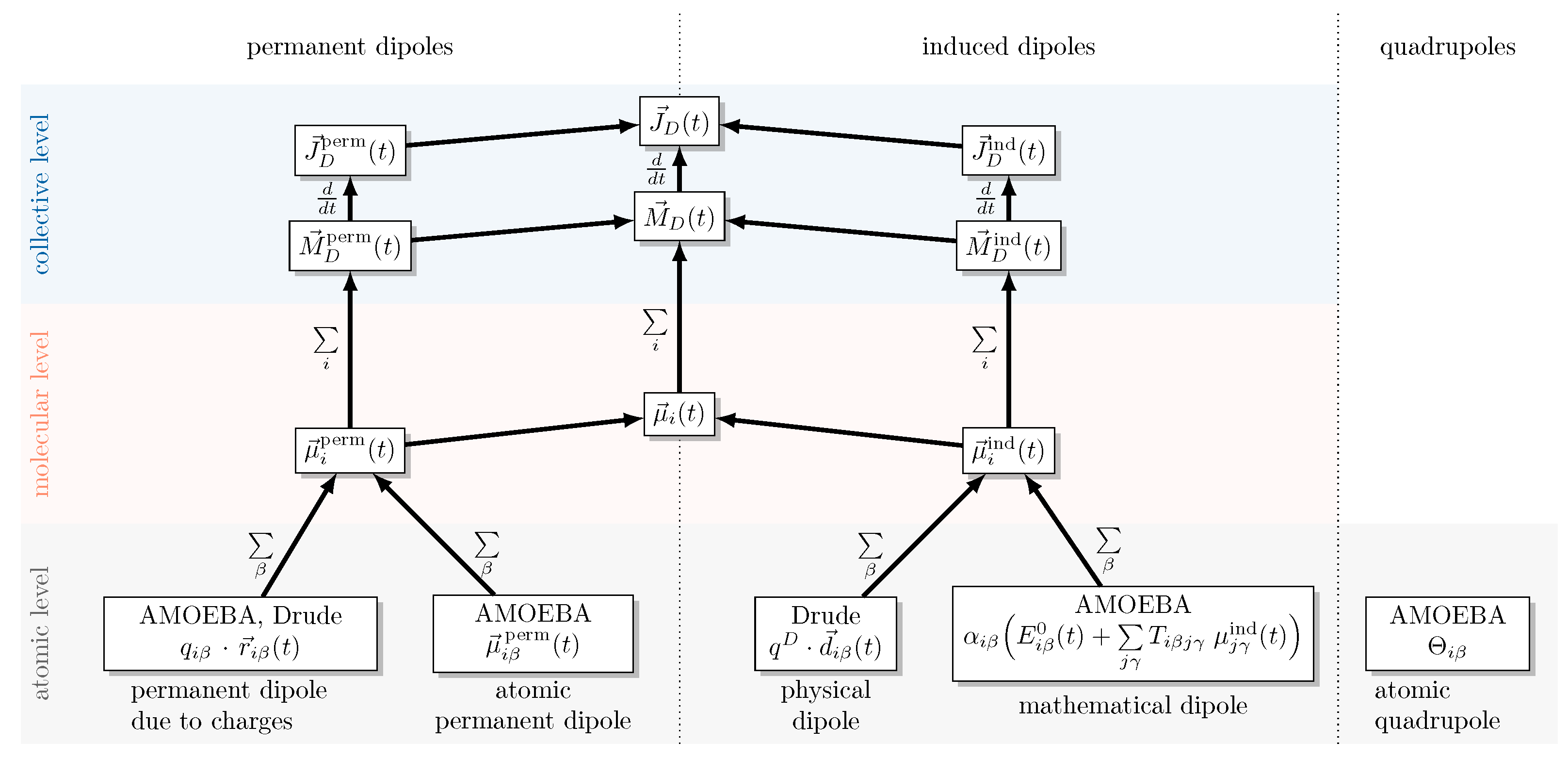
2.2. Decomposition of the Dipole Moment
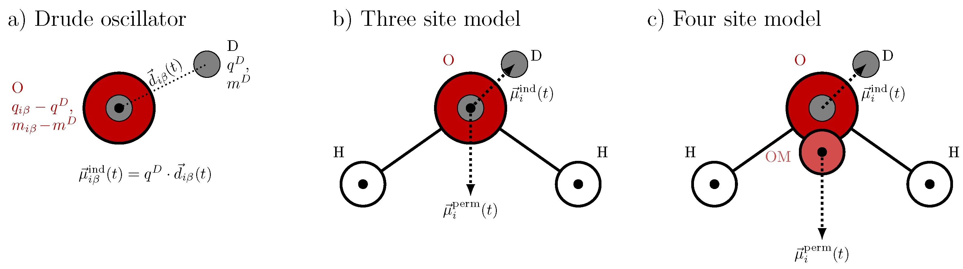
2.3. Drude Polarizable Water Models
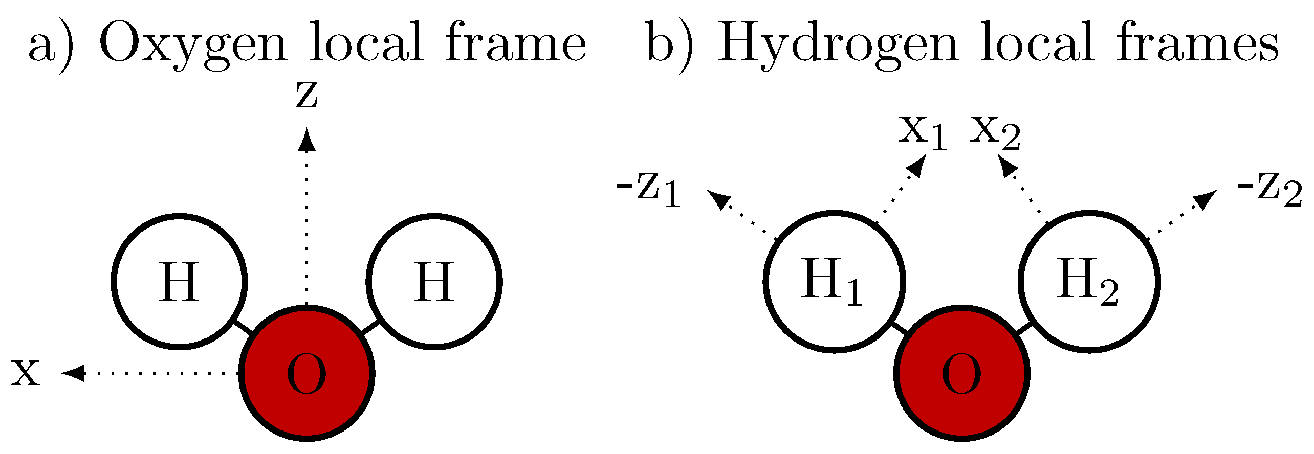
2.4. Amoeba Water Models Using Multipoles
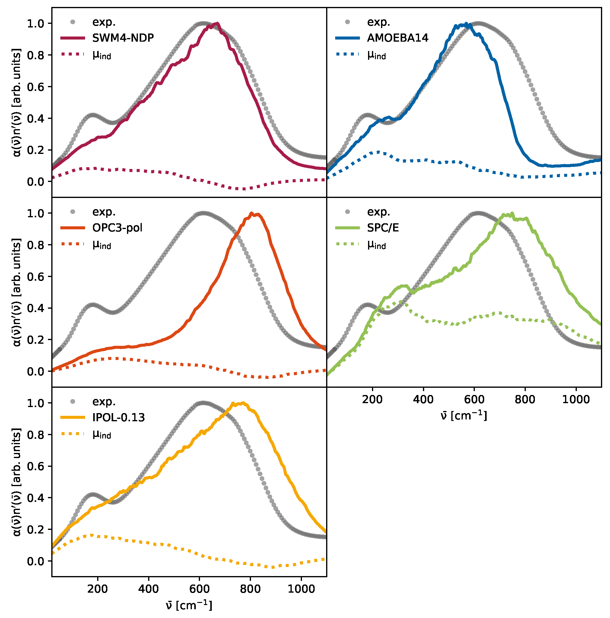
3. Results and Discussion
3.1. The Marginal Impact of Charge Transfer
3.2. The Importance of Polarization
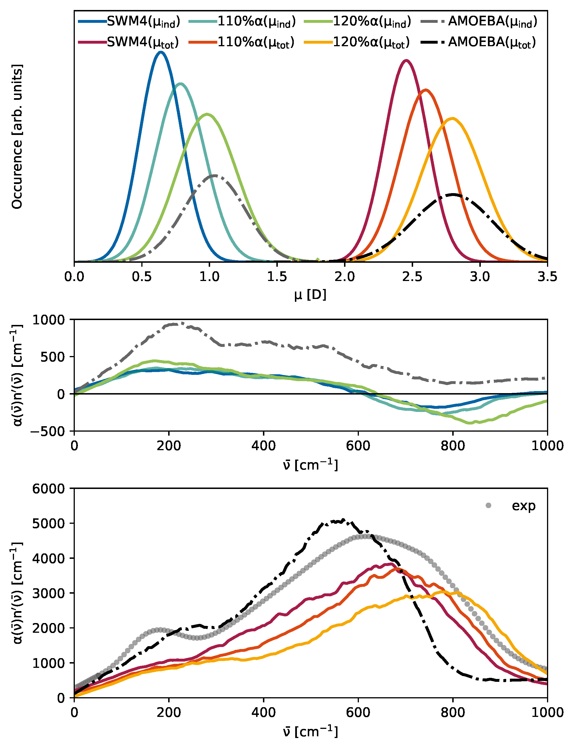
3.3. The Competition Between Induced and Permanent Dipoles
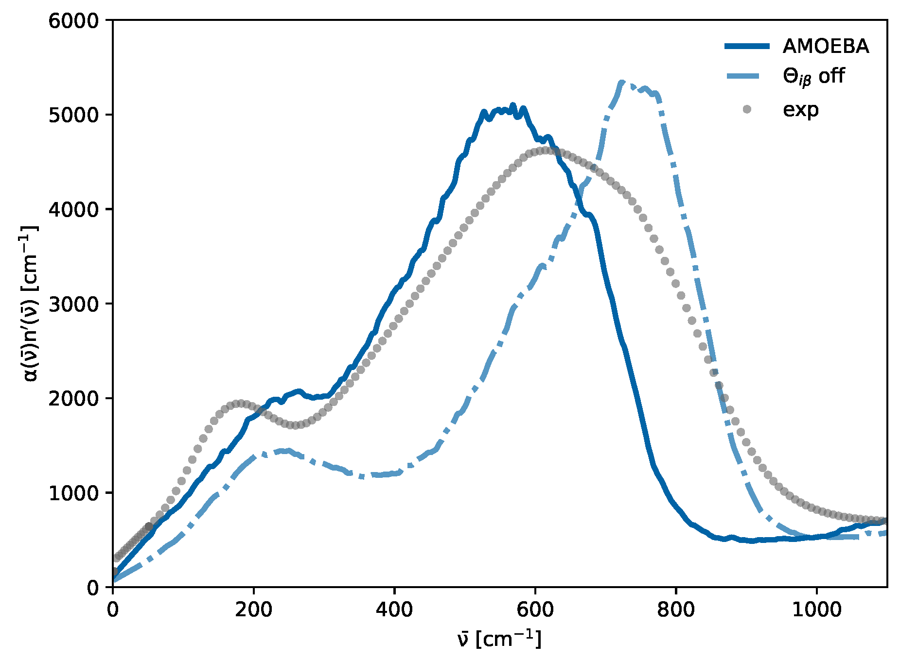
3.4. Cross- and Self-Terms
3.5. Dipole Moments
4. Conclusions
Supplementary Materials
Author Contributions
Funding
Institutional Review Board Statement
Informed Consent Statement
Data Availability Statement
Acknowledgments
Conflicts of Interest
References
- Wulf, A.; Fumino, K.; Ludwig, R.; Taday, P.F. Combined THz, FIR and Raman Spectroscopy Studies of Imidazolium-Based Ionic Liquids Covering the Frequency Range 2–300 cm−1. Chem. Phys. Chem. 2010, 11, 349–353. [Google Scholar] [CrossRef] [PubMed]
- Zasetsky, A.Y.; Lileev, A.S.; Lyashchenko, A.K. Molecular dynamic simulations of terahertz spectra for water-methanol mixtures. Mol. Phys. 2010, 108, 649–656. [Google Scholar] [CrossRef]
- Cherkasova, O.; Nazarov, M.; Konnikova, M.; Shkurinov, A. THz spectroscopy of bound water in glucose: Direct measurements from crystalline to dissolved state. J. Infrared Millim. 2020, 41, 1057–1068. [Google Scholar] [CrossRef]
- Ruiz-Barragan, S.; Sebastiani, F.; Schienbein, P.; Abraham, J.; Schwaab, G.; Nair, R.R.; Havenith, M.; Marx, D. Nanoconfinement effects on water in narrow graphene-based slit pores as revealed by THz spectroscopy. Phys. Chem. Chem. Phys. 2022, 24, 24734–24747. [Google Scholar] [CrossRef]
- Pyne, P.; Mahanta, D.D.; Gohil, H.; Prabhu, S.; Mitra, R.K. Correlating solvation with conformational pathways of proteins in alcohol–water mixtures: A THz spectroscopic insight. Phys. Chem. Chem. Phys. 2021, 23, 17536–17544. [Google Scholar] [CrossRef] [PubMed]
- Fei, S.; Hsu, W.L.; Delaunay, J.J.; Daiguji, H. Molecular dynamics study of water confined in MIL-101 metal–organic frameworks. J. Chem. Phys. 2021, 154, 144503. [Google Scholar] [CrossRef]
- Sega, M.; Schröder, C. Dielectric and terahertz spectroscopy of polarizable and nonpolarizable water models: A comparative study. J. Phys. Chem. A 2015, 119, 1539–1547. [Google Scholar] [CrossRef]
- Grechko, M.; Hasegawa, T.; D’Angelo, F.; Ito, H.; Turchinovich, D.; Nagata, Y.; Bonn, M. Coupling between intra- and intermolecular motions in liquid water revealed by twodimensional terahertz-infrared-visible spectroscopy. Nat. Commun. 2018, 9, 885. [Google Scholar] [CrossRef] [PubMed]
- Novelli, F.; Pestana, L.R.; Bennett, K.C.; Sebastiani, F.; Adams, E.M.; Stavrias, N.; Ockelmann, T.; Colchero, A.; Hoberg, C.; Schwaab, G.; et al. Strong Anisotropy in Liquid Water upon Librational Excitation Using Terahertz Laser Fields. J. Phys. Chem. B 2020, 124, 4989–5001. [Google Scholar] [CrossRef]
- Novelli, F.; Hoberg, C.; Adams, E.M.; Klopf, J.M.; Havenith, M. Terahertz pump–probe of liquid water at 12.3 THz. Phys. Chem. Chem. Phys. 2022, 24, 653–665. [Google Scholar] [CrossRef]
- Laage, D.; Elsaesser, T.; Hynes, J.T. Water Dynamics in the Hydration Shells of Biomolecules. Chem. Rev. 2017, 117, 10694–10725. [Google Scholar] [CrossRef] [PubMed]
- Williams, G.P. Filling the THz gap—high power sources and applications. Rep. Prog. Phys. 2005, 69, 301. [Google Scholar] [CrossRef]
- Perakis, F.; De Marco, L.; Shalit, A.; Tang, F.; Kann, Z.R.; Kühne, T.D.; Torre, R.; Bonn, M.; Nagata, Y. Vibrational Spectroscopy and Dynamics of Water. Chem. Rev. 2016, 116, 7590–7607. [Google Scholar] [CrossRef]
- Hasted, J.B.; Husain, S.K.; Frescura, F.A.M.; Birch, J.R. Far-infrared absorption in liquid water. Chem. Phys. Lett. 1985, 118, 622–625. [Google Scholar] [CrossRef]
- Chakraborty, S.; Sinha, S.K.; Bandyopadhyay, S. Low-Frequency Vibrational Spectrum of Water in the Hydration Layer of a Protein: A Molecular Dynamics Simulation Study. J. Phys. Chem. B 2007, 111, 13626–13631. [Google Scholar] [CrossRef] [PubMed]
- Heyden, M.; Havenith, M. Combining THz spectroscopy and MD simulations to study protein-hydration coupling. Methods 2010, 52, 74–83. [Google Scholar] [CrossRef]
- Inagaki, T.; Hatanaka, M.; Saito, S. Anisotropic and Finite Effects on Intermolecular Vibration and Relaxation Dynamics: Low-Frequency Raman Spectroscopy of Water Film and Droplet on Graphene by Molecular Dynamics Simulations. J. Phys. Chem. B 2023, 127, 5869–5880. [Google Scholar] [CrossRef]
- Torii, H. Simulations of the THz spectrum of liquid water incorporating the effects of the intermolecular charge fluxes through hydrogen bonds. AIP Conf. Proc. 2015, 1702, 090043. [Google Scholar]
- Chen, W.; Sharma, M.; Resta, R.; Galli, G.; Car, R. Role of dipolar correlations in the infrared specra of water and ice. Phys. Rev. B 2008, 77, 245114. [Google Scholar] [CrossRef]
- Heyden, M.; Sun, J.; Funkner, S.; Mathias, G.; Forbert, H.; Havenith, M.; Marx, D. Dissecting the THz spectrum of liquid water from first principles via correlations in time and space. Proc. Natl. Acad. Sci. USA 2010, 107, 12068–12073. [Google Scholar] [CrossRef]
- Carlson, S.; Brünig, F.N.; Loche, P.; Bonthuis, D.J.; Netz, R.R. Exploring the absorption spectrum of simulated water from MHz to Infrared. J. Phys. Chem. A 2020, 124, 5599. [Google Scholar] [CrossRef] [PubMed]
- Madden, P.A.; Impey, R.W. On the infrared and Raman spectra of water in the region 5–250 cm−1. Chem. Phys. Lett. 1986, 123, 502–506. [Google Scholar] [CrossRef]
- Demerdash, O.; Wang, L.P.; Head-Gordon, T. Advanced models for water simulations. WIREs Comput Mol Sci 2018, 8, e1355. [Google Scholar] [CrossRef]
- Babin, V.; Medders, G.R.; Paesani, F. Development of a “First Principles” Water Potential with Flexible Monomers. II: Trimer Potential Energy Surface, Third Virial Coefficient, and Small Clusters. J. Chem. Theory Comput. 2014, 10, 1599–1607. [Google Scholar] [CrossRef] [PubMed]
- Joerg, F.; Wieder, M.; Schröder, C. Protex—A Python utility for proton exchange in molecular dynamics simulations. Front. Chem. Sec. Mol. Liq. 2023, 11, 1140896. [Google Scholar] [CrossRef]
- Gődény, M.; Joerg, F.; Kovar, M.P.P.; Schröder, C. Updates to Protex for Simulating Proton Transfers in an Ionic Liquid. J. Phys. Chem. B 2024, 128, 3416–3426. [Google Scholar] [CrossRef] [PubMed]
- Sharma, M.; Resta, R.; Car, R. Intermolecular Dynamical Charge Fluctuations in Water: A Signature of the H-Bond Network. Phys. Rev. Lett. 2005, 95, 187401. [Google Scholar] [CrossRef]
- Sharma, D.; Das, B.; Chandra, A. Terahertz Spectrum of Water at Varying Temperatures from 260 to 340 K: Contributions from Permanent and Induced Dipole Correlations at Different Length Scales. J. Phys. Chem. B 2023, 127, 6714–6725. [Google Scholar] [CrossRef]
- Han, B.; Isborn, C.M.; Shi, L. Incorporating Polarization and Charge Transfer into a Point-Charge Model for Water Using Machine Learning. J. Phys. Chem. Lett. 2023, 14, 3869–3877. [Google Scholar] [CrossRef]
- Berendsen, H.J.C.; Grigera, J.R.; Straatsma, T.P. The Missing Term in Effective Pair Potentials. J. Phys. Chem. 1987, 91, 6269. [Google Scholar] [CrossRef]
- Abascal, J.L.F.; Vega, C. A general purpose model for the condensed phases of water: TIP4P/2005. J. Chem. Phys. 2005, 123, 234505. [Google Scholar] [CrossRef] [PubMed]
- Wu, Y.; Tepper, H.L.; Voth, G.A. Flexible simple point-charge water model with improved liquid-state properties. J. Chem. Phys. 2006, 124, 024503. [Google Scholar] [CrossRef] [PubMed]
- González, M.A.; Abascal, J.L.F. A flexible model for water based on TIP4P/2005. J. Chem. Phys. 2004, 135, 224516. [Google Scholar] [CrossRef]
- Hamm, P. 2D-Raman-THz spectroscopy: A sensitive test of polarizable water models. J. Chem. Phys. 2014, 141, 184201. [Google Scholar] [CrossRef]
- Shi, L.; Ni, Y.; Drews, S.E.P.; Skinner, J.L. Dielectric constant and low-frequency infrared spectra for liquid water and ice Ih within the E3B model. J. Chem. Phys. 2014, 141, 084508. [Google Scholar] [CrossRef] [PubMed]
- Lamoureux, G.; Harder, E.; Vorobyov, I.V.; Roux, B.; MacKerell, A.D. A polarizable model of water for molecular dynamics simulations of biomolecules. Chem. Phys. Lett. 2006, 418, 245–249. [Google Scholar] [CrossRef]
- Sidler, D.; Meuwly, M.; Hamm, P. An efficient water force field calibrated against intermolecular THz and Raman spectra. J. Chem. Phys. 2018, 148, 244504. [Google Scholar] [CrossRef]
- Tröster, P.; Lorenzen, K.; Schwörer, M.; Tavan, P. Polarizable Water Models from Mixed Computational and Empirical Optimization. J. Phys. Chem. B 2013, 117, 9486–9500. [Google Scholar] [CrossRef]
- Xiong, Y.; Izadi, S.; Onufriev, A.V. Fast Polarizable Water Model for Atomistic Simulations. J. Chem. Theory Comput. 2022, 18, 6324–6333. [Google Scholar] [CrossRef]
- Kolafa, J. A Polarizable Three-Site Water Model with Intramolecular Polarizability. Collect. Czech. Chem. Commun. 2008, 73, 507–517. [Google Scholar] [CrossRef]
- Liu, C.; Piquemal, J.P.; Ren, P. Implementation of Geometry-Dependent Charge Flux into the Polarizable AMOEBA+ Potential. J. Phys. Chem. Lett. 1957, 11, 419–426. [Google Scholar] [CrossRef]
- Laury, M.L.; Wang, L.P.; Pande, V.S.; Head-Gordon, T.; Ponder, J.W. Revised Parameters for the AMOEBA Polarizable Atomic Multipole Water Model. J. Phys. Chem. B 2015, 119, 9423–9437. [Google Scholar] [CrossRef]
- Wang, L.P.; Head-Gordon, T.; Ponder, J.W.; Ren, P.; Chodera, J.D.; Eastman, P.K.; Martinez, T.J.; Pande, V.S. Systematic Improvement of a Classical Molecular Model of Water. J. Phys. Chem. B 2013, 117, 9956–9972. [Google Scholar] [CrossRef]
- Liu, C.; Piquemal, J.P.; Ren, P. AMOEBA+ Classical Potential for Modeling Molecular Interactions. J. Chem. Theory Comput. 2019, 15, 4122–4139. [Google Scholar] [CrossRef]
- Hasegawa, T.; Tanimura, Y. A Polarizable Water Model for Intramolecular and Intermolecular Vibrational Spectroscopies. J. Phys. Chem. B 2011, 115, 5545–5553. [Google Scholar] [CrossRef]
- Liu, J.; Miller, W.H.; Fanourgakis, G.S.; Xantheas, S.S.; Imoto, S.; Saito, S. Insights in quantum dynamical effects in the infrared spectroscopy of liquid water from a semiclassical study with an ab initio-based flexible and polarizable force field. J. Chem. Phys. 2011, 135, 244503. [Google Scholar] [CrossRef]
- Fanourgakis, G.S.; Xantheas, S.S. Development of transferable interaction potentials for water. V. Extension of the flexible, polarizable, Thole-type model potential TTM3-F, v. 3.0 to describe the vibrational spectra of water clusters and liquid water. J. Chem. Phys. 2008, 128, 074506. [Google Scholar] [CrossRef]
- Torii, H. Cooperative Contributions of the Intermolecular Charge Fluxes and Intramolecular Polarizations in the Far-Infrared Spectral Intensities of Liquid Water. J. Chem. Theory Comput. 2014, 10, 1219–1227. [Google Scholar] [CrossRef]
- Medders, G.R.; Paesani, F. Infrared and Raman Spectroscopy of Liquid Water through “First-Principles” Many-Body Molecular Dynamics. J. Chem. Theory Comput. 2015, 11, 1145–1154. [Google Scholar] [CrossRef]
- Liu, H.; Wang, Y.; Bowman, J.M. Quantum calculations of the IR spectrum of liquid water using ab initio and model potential and dipole moment surfaces and comparison with experiment. J. Chem. Phys. 2015, 142, 194502. [Google Scholar] [CrossRef]
- Elton, D.C.; Fernández-Serra, M.V. Polar nanoregions in water: A study of the dielectric properties of TIP4P/2005, TIP4P/2005f and TTM3F. J. Chem. Phys. 2014, 140, 124504. [Google Scholar] [CrossRef] [PubMed]
- Stukan, M.R.; Asmadi, A.; Abdallah, W. Bulk properties of SWM4-NDP water model at elevated temperature and pressure. J. Mol. Liq. 2013, 180, 65–69. [Google Scholar] [CrossRef]
- Malmberg, C.; Maryott, A. Dielectric constant of water from 0 to 100 C. J. Res. Natl. Inst. Stand. Technol. 1956, 56, 1–8. [Google Scholar] [CrossRef]
- Esser, A.; Belsare, S.; Marx, D.; Head-Gordon, T. Mode specific THz spectra of solvated amino acids using the AMOEBA polarizable force field. Phys. Chem. Chem. Phys. 2017, 19, 5579–5590. [Google Scholar] [CrossRef]
- Case, D.A.; Aktulga, H.M.; Belfon, K.; Cerutti, D.S.; Cisneros, G.A.; Cruzeiro, V.W.D.; Forouzesh, N.; Giese, T.J.; Götz, A.W.; Gohlke, H.; et al. AmberTools. J. Chem. Inf. Model 2023, 63, 6183–6191. [Google Scholar] [CrossRef]
- Rackers, J.A.; Wang, Z.; Lu, C.; Laury, M.L.; Lagardere, L.; Schnieders, M.J.; Piquemal, J.P.; Ren, P.; Ponder, J. Tinker 8: Software Tools for Molecular Desig. J. Chem. Theory Comput. 2018, 14, 5273–5289. [Google Scholar] [CrossRef]
- Eastman, P.; Swails, J.; Chodera, J.D.; McGibbon, R.T.; Zhao, Y.; Beauchamp, K.A.; Wang, L.P.; Simmonett, A.C.; Harrigan, M.P.; Stern, C.D.; et al. OpenMM 7: Rapid development of high performance algorithms for molecular dynamics. PLoS Comput. Biol. 2017, 13, e1005659. [Google Scholar] [CrossRef]
- Wooten, F. Optical Properties of Solids; Academic Press: New York, NY, USA; London, UK, 1972. [Google Scholar]
- Schröder, C.; Steinhauser, O. Using fit functions in computational dielectric spectroscopy. J. Chem. Phys. 2010, 132, 244109. [Google Scholar] [CrossRef]
- Thomas, M.; Brehm, M.; Fligg, R.; Vöhringer, P.; Kirchner, B. Computing vibrational spectra from ab initio molecular dynamics. Phys. Chem. Chem. Phys. 2013, 15, 6608–6622. [Google Scholar] [CrossRef]
- Szabadi, A.; Doknic, A.; Netsch, J.; Palvögyi, A.M.; Steinhauser, O.; Schröder, C. Force field refinement for reproducing experimental infrared spectra of ionic liquids. Phys. Chem. Chem. Phys. 2023, 25, 19882–19890. [Google Scholar] [CrossRef]
- Mauger, N.; Plé, T.; Lagardère, L.; Huppert, S.; Piquemal, J.P. Improving Condensed-Phase Water Dynamics with Explicit Nuclear Quantum Effects: The Polarizable Q-AMOEBA Force Field. J. Phys. Chem. B 2022, 126, 8813–8826. [Google Scholar] [CrossRef]
- Flór, M.; Wilkins, D.M.; de la Puente, M.; Laage, D.; Cassone, G.; Hassanali, A.; Roke, S. Dissecting the hydrogen bond network of water:Charge transfer and nuclear quantum effects. Science 2024, 386, 1110. [Google Scholar] [CrossRef] [PubMed]
- Machida, M.; Kato, K.; Shiga, M. Nuclear quantum effects of light and heavy water studied by all-electron first principles path integral simulations. J. Chem. Phys. 2017, 148, 102324. [Google Scholar] [CrossRef]
- Stone, A.J. The Theory of Intermolecular Forces; Clarendon Press: Oxford, UK, 1996. [Google Scholar]
- Devereux, M.; Pezzella, M.; Raghunathan, S.; Meuwly, M. Polarizable Multipolar Molecular Dynamics Using Distributed Point Charges. J. Chem. Theory Comput. 2020, 16, 7267–7280. [Google Scholar] [CrossRef]
- Gray, C.G. Spherical tensor approach to multipole expansions. I. Electrostatic interaction. Can. J. Phys. 1975, 54, 505–512. [Google Scholar] [CrossRef]
- Pan, C.; Liu, C.; Peng, J.; Ren, P.; Huang, X. Three-site and five-site fixed-charge water models compatiblewith AMOEBA force field. J. Comput. Chem. 2020, 41, 1034–1044. [Google Scholar] [CrossRef] [PubMed]
- Ren, P.Y.; Ponder, J.W. Polarizable Atomic Multipole Water Model for Molecular Mechanics Simulation. J. Phys. Chem. B 2003, 107, 5933–5947. [Google Scholar] [CrossRef]
- Torabifard, H.; Starovoytov, O.N.; Ren, P.; Cisneros, G.A. Development of an AMOEBA water model using GEM distributed multipoles. Theor. Chem. Acc. 2015, 134, 101. [Google Scholar] [CrossRef]
- Das, A.K.; Demerdash, O.N.; Head-Gordon, T. Improvemnets to the AMOEBA Force Field by Introducing Anisotropic Atomic Polarizability of the Water Molecule. J. Chem. Theory Comput. 2018, 14, 6722–6733. [Google Scholar] [CrossRef]
- Rick, S.W.; Stuart, S.J.; Berne, B.J. Dynamical fluctuating charge force fields: Application to liquid water. J. Chem. Phys. 1994, 101, 6141–6156. [Google Scholar] [CrossRef]
- Rick, S.W.; Berne, B.J. Free Energy of the Hydrophobic Interaction from Molecular Dynamics Simulations: The Effects of Solute and Solvent Polarizability. J. Phys. Chem. B 1997, 101, 10488–10493. [Google Scholar] [CrossRef]
- Rick, S.W. Simulations of ice and liquid water over a range of temperatures using the fluctuating charge model. J. Chem. Phys. 2001, 114, 2276–2283. [Google Scholar] [CrossRef]
- Vácha, R.; Marsalek, O.; Willard, A.P.; Bonthuis, D.J.; Netz, R.R.; Jungwirth, P. Charge Transfer between Water Molecules As the Possible Origin of the Observed Charging at the Surface of Pure Water. J. Phys. Chem. Lett. 2012, 3, 107–111. [Google Scholar] [CrossRef]
- Roncaratti, L.F.; Belpassi, L.; Cappelletti, D.; Pirani, F.; Tarantelli, F. Molecular-Beam Scattering Experiments and Theoretical Calculations Probing Charge Transfer in Weakly Bound Complexes of Water. J. Phys. Chem. A 2009, 113, 15223–15232. [Google Scholar] [CrossRef]
- Marenich, A.V.; Cramer, C.J.; Truhlar, D.G. Universal Solvation Model Based on Solute Electron Density and on a Continuum Model of the Solvent Defined by the Bulk Dielectric Constant and Atomic Surface Tensions. J. Phys. Chem. B 2009, 113, 6378–6396. [Google Scholar] [CrossRef]
- Martin, F.; Zipse, H. Charge distribution in the water molecule—A comparison of methods. J. Comput. Chem. 2005, 26, 97–105. [Google Scholar] [CrossRef]
- Han, B.; Isborn, C.M.; Shi, L. Determining Partial Atomic Charges for Liquid Water: Assessing Electronic Structure and Charge Models. J. Chem. Theory Comput. 2021, 17, 889–901. [Google Scholar] [CrossRef] [PubMed]
- Ghosh, S.R.; Debnath, B.; Jana, A.D. Water dimer isomers: Interaction energies and electronic structure. J. Mol. Model. 2020, 26, 20. [Google Scholar] [CrossRef]
- Baker, C.M.; MacKerell, A.D., Jr. Polarizability rescaling and atom-based Thole scaling in the CHARMM Drude polarizable force field for ethers. J. Mol. Model. 2010, 16, 567–576. [Google Scholar] [CrossRef]
- Bertie, J.E.; Lan, Z. Infrared Intensities of Liquids XX: The Intensity of the OH Stretching Band of Liquid Water Revisited, and the Best Current Values of the Optical Constants of H2O(l) at 25 °C between 15,000 and 1 cm−1. Appl. Spectrosc. 1996, 50, 1047–1057. [Google Scholar] [CrossRef]
- Martinez, L.; Andrade, R.; Birgin, E.G.; Martinez, J.M. Packmol: A package for building initial configurations for molecular dynamics simulations. J. Comput. Chem. 2009, 30, 2157–2164. [Google Scholar] [CrossRef] [PubMed]
- Brooks, B.R.; Brooks, C.L., III; MacKerell, A.D., Jr.; Nilsson, L.; Petrella, R.J.; Roux, B.; Won, Y.; Archontis, G.; Bartels, C.; Boresch, S.; et al. CHARMM: The biomolecular simulation program. J. Comput. Chem. 2009, 30, 1545–1614. [Google Scholar] [CrossRef] [PubMed]
- Liu, D.C.; Nocedal, J. On the limited memory BFGS method for large scale optimization. Math. Program. 1989, 45, 503–528. [Google Scholar] [CrossRef]
- Michaud-Agrawal, N.; Denning, E.J.; Woolf, T.B.; Beckstein, O. MDAnalysis: A Toolkit for the Analysis of Molecular Dynamics Simulations. J. Comput. Chem. 2011, 32, 2319–2327. [Google Scholar] [CrossRef]
- Gowers, R.J.; Linke, M.; Barnoud, J.; Reddy, T.J.E.; Melo, M.N.; Seyler, S.L.; Dotson, D.L.; Domanski, J.; Buchoux, S.; Kenney, I.M.; et al. MDAnalysis: A Python package for the rapid analysis of molecular dynamics simulations. In Proceedings of the 15th Python in Science Conference, Austin, TX, USA, 11–17 July 2016; pp. 102–109. [Google Scholar]


| Water Model | Reference | H-O-H Angle a [deg] | 200 cm−1 |
|---|---|---|---|
| Rigid, non-polarizable | |||
| SPC/E | [29] | 109.47 [30] | no |
| TIP4P/2005 | [29] | 104.52 [31] | no |
| Flexible, non-polarizable | |||
| SPC/Fw | [32] | 113.24 [32] | no |
| TIP4P/2005f | [29] | 107.4 [33] | no |
| Rigid, with post-MD induced dipoles | |||
| SPC/E- | this work | 109.47 | yes |
| TIP4P/2005- | [34] | 104.52 | yes |
| E3B- | [35] | 104.52 | shoulder |
| Rigid, polarizable | |||
| SWM4-NDP | This work, [34] | 104.52 [36] | shoulder |
| SWM4-NDP+10%pol. | This work | 104.52 | shoulder |
| SWM4-NDP+20%pol. | This work | 104.52 | yes |
| TL4P | [37] | 105.3 b [38] | shoulder |
| OPC3-pol | This work | 109.47 [39] | shoulder |
| IPOL-0.13 | This work | 109.47 [40] | shoulder |
| Flexible, polarizable | |||
| AMOEBA14 | This work, [9,23,28,41] | 107.91 [42] | yes |
| AMOEBA14 ( off) | This work | 107.91 | yes |
| iAMOEBA | [43] | 106.48 [43] | yes |
| AMOEBA+ | [41] | 108.81 [44] | yes |
| Flexible, polarizable with charge flux | |||
| POLI2VS | [45] | 104.52 [45] | yes |
| AMOEBA+CF | [41] | 104.54 [41] | shoulder |
| TTM3-F | [46] | 104.5078 [47] | shoulder |
| Rigid, polarizable with charge transfer | |||
| TL4Pi-CT | [37] | 105.3 b [38] | yes |
| TIP4P-/CT | [48] | 104.52 | yes |
| Explicit, many-body potential | |||
| MB-pol | [49] | 104.69 c [24] | yes |
| WHBB | [50] | - d | yes |
| Atom Type | ||||
|---|---|---|---|---|
| [e] | [D] | [D Å] | [D] | |
| SPC/E [30] | ||||
| OT | −0.848 | 2.36 | ||
| HT | 0.424 | |||
| SWM4 [36] | ||||
| O | 0.00000 | |||
| OM | −1.11466 | 1.85 | ||
| H | 0.55733 | |||
| IPOL-0.13 [40] | ||||
| O | −0.669 | 1.86 | ||
| H | 0.3345 | |||
| OPC3-pol [39] | ||||
| O | −0.610 | 2.05 | ||
| H | 0.305 | |||
| AMOEBA14 [42] | ||||
| O | −0.42616 | = 0.236 | 1.71 | |
| z = 0.159 | = −0.312 | |||
| = 0.075 | ||||
| H | 0.21308 | x = −0.257 | = 0.165 | |
| = 0.120 | ||||
| z = −0.691 | = −0.094 | |||
| = −0.286 | ||||
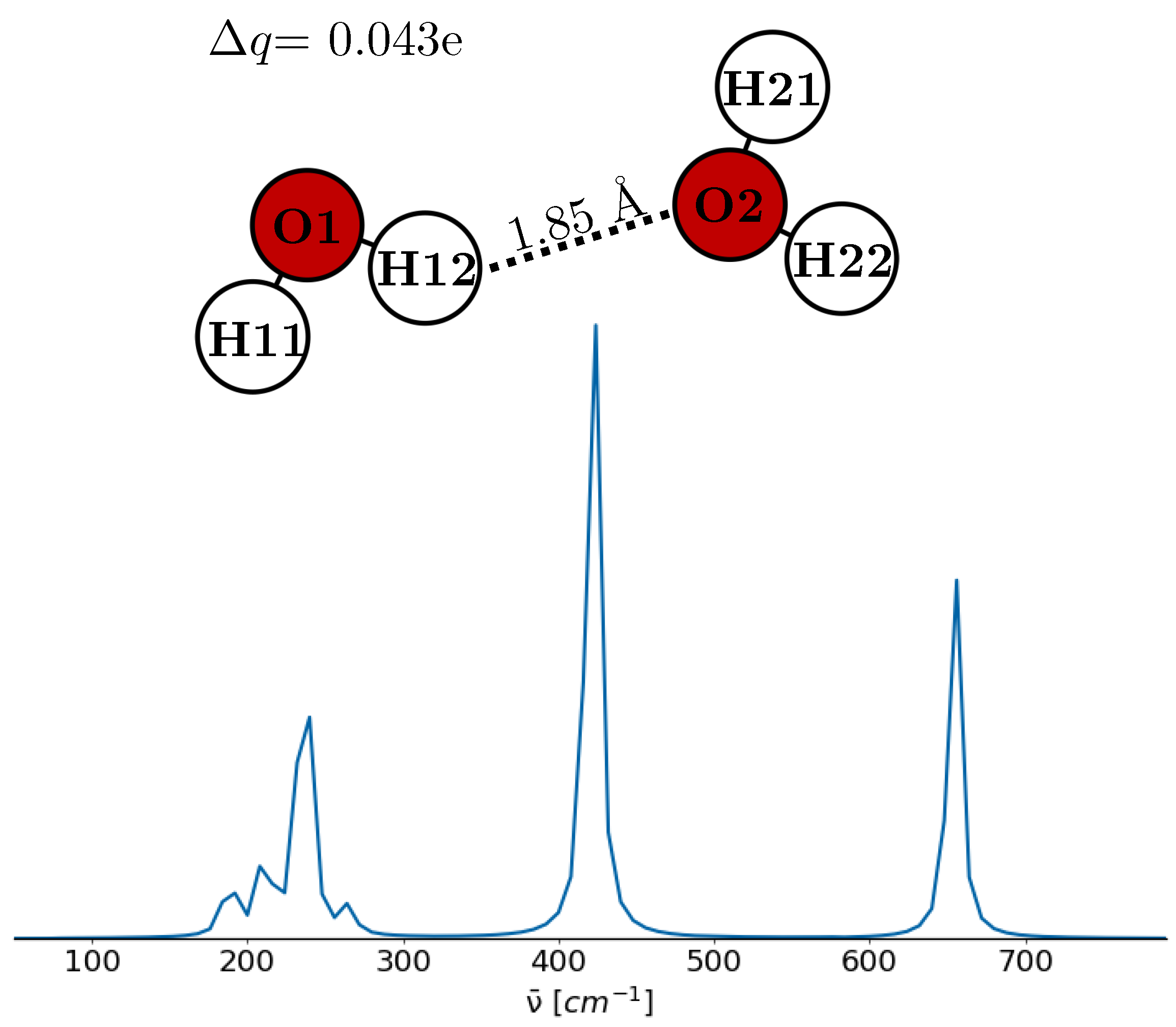
| Water dimer | ||||
| O1 | −0.810 | |||
| H11 | 0.384 | 2.37 | ||
| H12 | 0.383 | |||
| O2 | −0.752 | |||
| H21 | 0.394 | 2.35 | ||
| H22 | 0.401 | |||
| Model | [D] | [D] | [D] |
|---|---|---|---|
| SPC/E (added polarizability) | 2.35 | 0.79 | 3.15 |
| SWM4-NDP | 1.85 | 0.65 | 2.50 |
| SWM4-NDP+10%pol. | 1.85 | 0.79 | 2.60 |
| SWM4-NDP+20%pol. | 1.85 | 0.99 | 2.80 |
| OPC3-pol | 2.05 | 1.09 | 3.11 |
| IPOL-0.13 | 1.86 | 1.22 | 3.05 |
| AMOEBA14 | 1.80 | 1.04 | 2.79 |
Disclaimer/Publisher’s Note: The statements, opinions and data contained in all publications are solely those of the individual author(s) and contributor(s) and not of MDPI and/or the editor(s). MDPI and/or the editor(s) disclaim responsibility for any injury to people or property resulting from any ideas, methods, instructions or products referred to in the content. |
© 2025 by the authors. Licensee MDPI, Basel, Switzerland. This article is an open access article distributed under the terms and conditions of the Creative Commons Attribution (CC BY) license (https://creativecommons.org/licenses/by/4.0/).
Share and Cite
Sappl, M.; Szabadi, A.; Honegger, P.; König, F.; Steinhauser, O.; Schröder, C. Insights from the Absorption Coefficient for the Development of Polarizable (Multipole) Force Fields. Molecules 2025, 30, 2941. https://doi.org/10.3390/molecules30142941
Sappl M, Szabadi A, Honegger P, König F, Steinhauser O, Schröder C. Insights from the Absorption Coefficient for the Development of Polarizable (Multipole) Force Fields. Molecules. 2025; 30(14):2941. https://doi.org/10.3390/molecules30142941
Chicago/Turabian StyleSappl, Marion, András Szabadi, Philipp Honegger, Franziska König, Othmar Steinhauser, and Christian Schröder. 2025. "Insights from the Absorption Coefficient for the Development of Polarizable (Multipole) Force Fields" Molecules 30, no. 14: 2941. https://doi.org/10.3390/molecules30142941
APA StyleSappl, M., Szabadi, A., Honegger, P., König, F., Steinhauser, O., & Schröder, C. (2025). Insights from the Absorption Coefficient for the Development of Polarizable (Multipole) Force Fields. Molecules, 30(14), 2941. https://doi.org/10.3390/molecules30142941