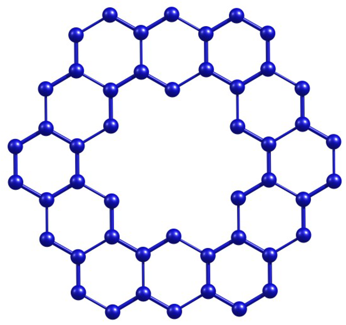
Figure 1.
Kekulene molecular structure.
Figure 1.
Kekulene molecular structure.
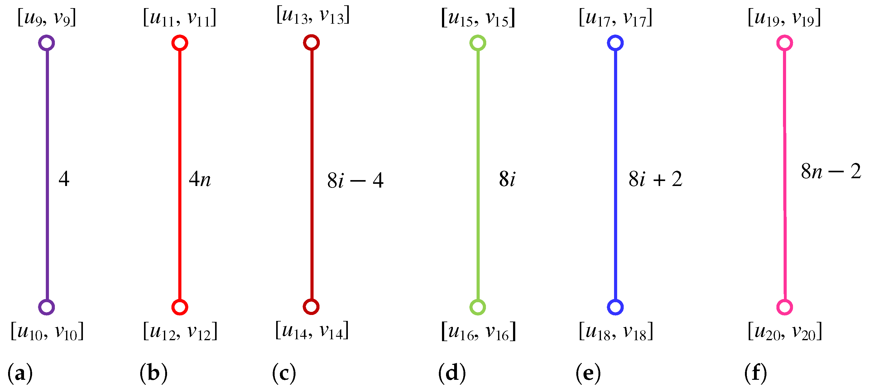
Figure 2.
(a) Zigzag Acute. (b) Zigzag Vertical. (c) Zigzag Obtuse. (d) Acute. (e) Horizontal. (f) Obtuse.
Figure 2.
(a) Zigzag Acute. (b) Zigzag Vertical. (c) Zigzag Obtuse. (d) Acute. (e) Horizontal. (f) Obtuse.
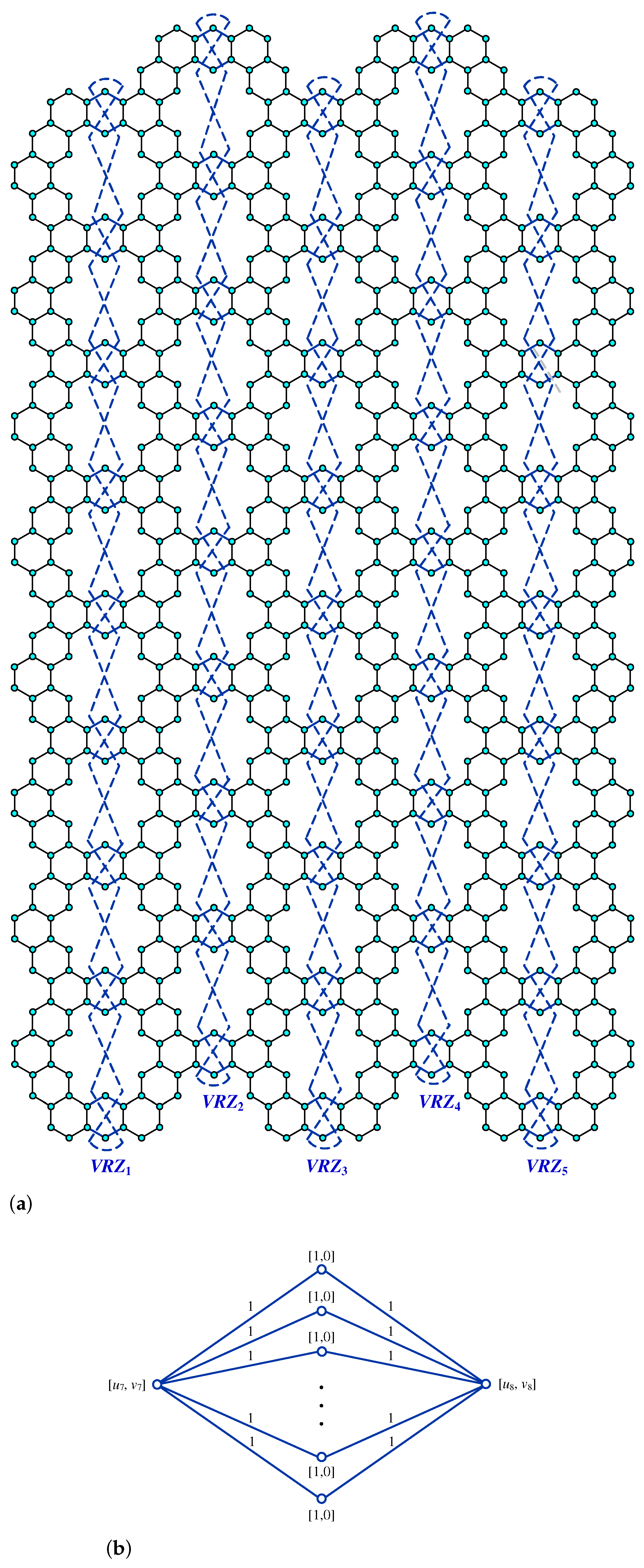
Figure 3.
(a) Kekulene Type-I. (b) Kekulene Type-II.
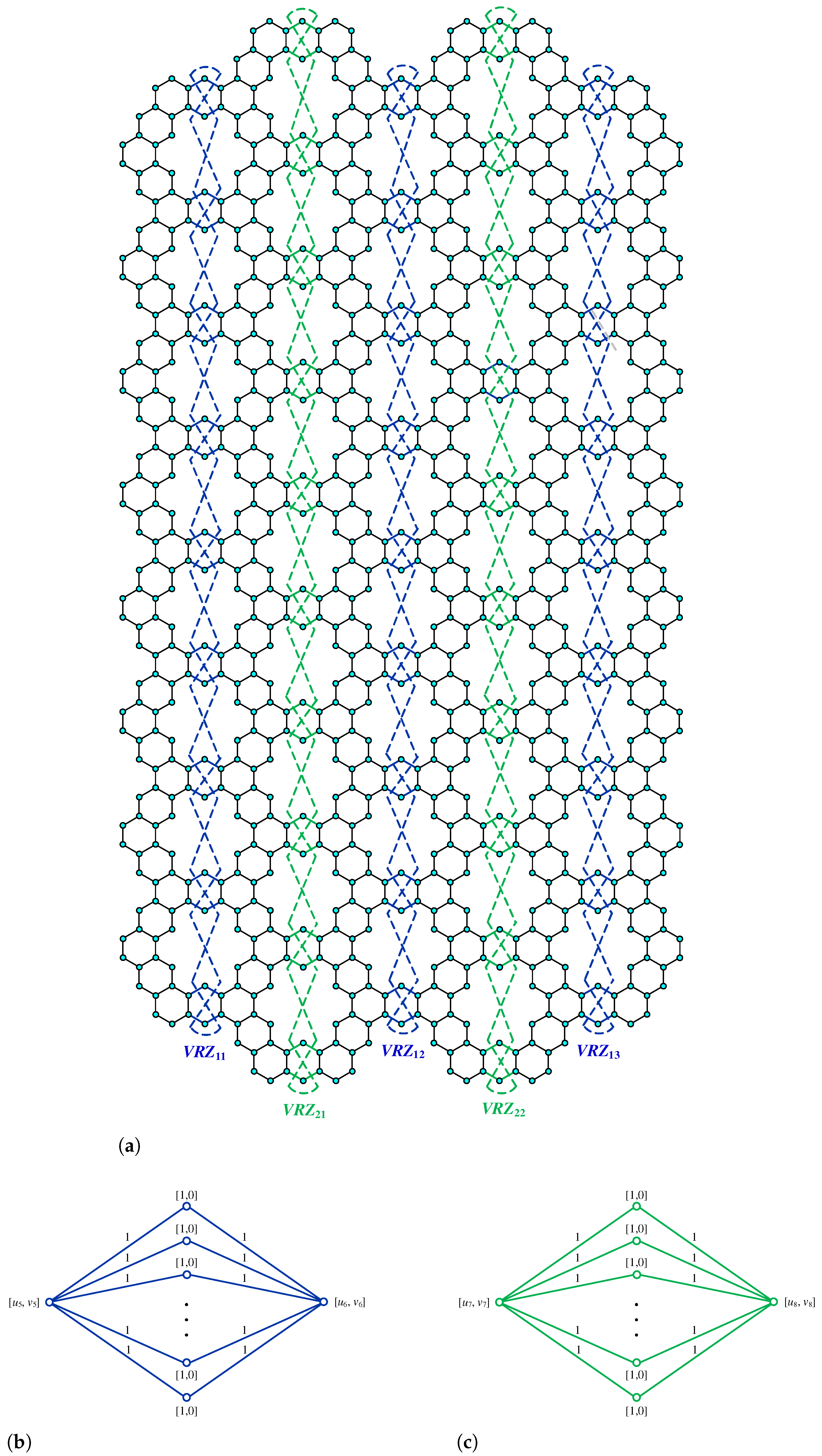
Figure 3.
(a) Kekulene Type-I. (b) Kekulene Type-II.
Figure 4.
(a) ; (b) ; (c) ; (d) .
Figure 4.
(a) ; (b) ; (c) ; (d) .
Figure 5.
, , , , , , and .
Figure 5.
, , , , , , and .
Figure 6.
(a) ; (b) ; (c) ; (d) ; (e) ; (f) ; (g) .
Figure 6.
(a) ; (b) ; (c) ; (d) ; (e) ; (f) ; (g) .
Figure 7.
(a) , ; (b) ; (c) ; (d) .
Figure 7.
(a) , ; (b) ; (c) ; (d) .
Figure 8.
(a) ; (b) .
Figure 8.
(a) ; (b) .
Figure 9.
(a) ; (b) ; (c) .
Figure 9.
(a) ; (b) ; (c) .
Figure 10.
(a) , , (b) , , , .
Figure 10.
(a) , , (b) , , , .
Figure 11.
(a) ; (b) ; (c) ; (d) ; (e) ; (f) .
Figure 11.
(a) ; (b) ; (c) ; (d) ; (e) ; (f) .
Figure 12.
(a) ; (b) ; (c) .
Figure 12.
(a) ; (b) ; (c) .
Figure 13.
Graphical representation of Type-I, .
Figure 13.
Graphical representation of Type-I, .
Figure 14.
Graphical representation of Type-II, .
Figure 14.
Graphical representation of Type-II, .
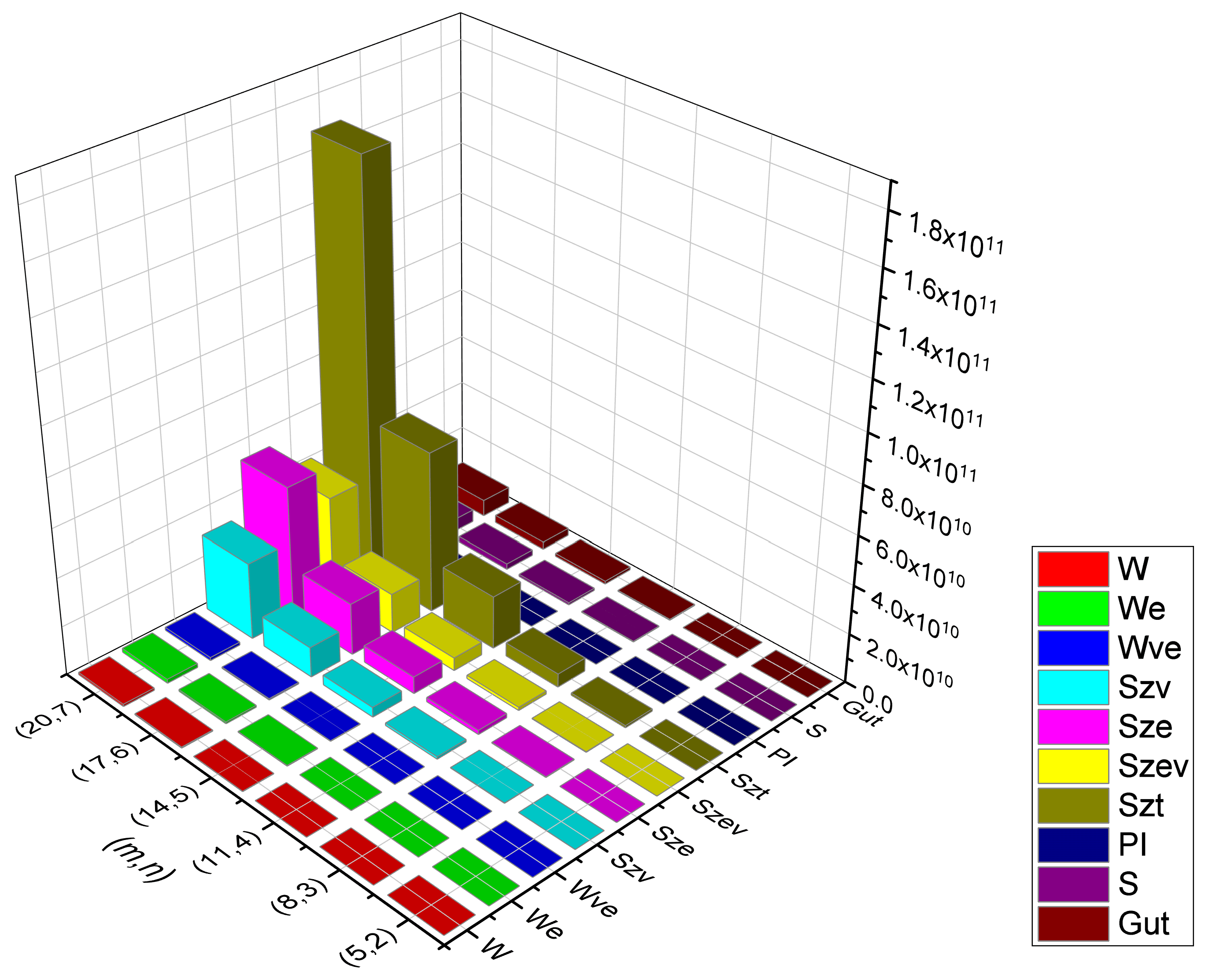
Figure 15.
Graphical representation of Type-I, .
Figure 15.
Graphical representation of Type-I, .
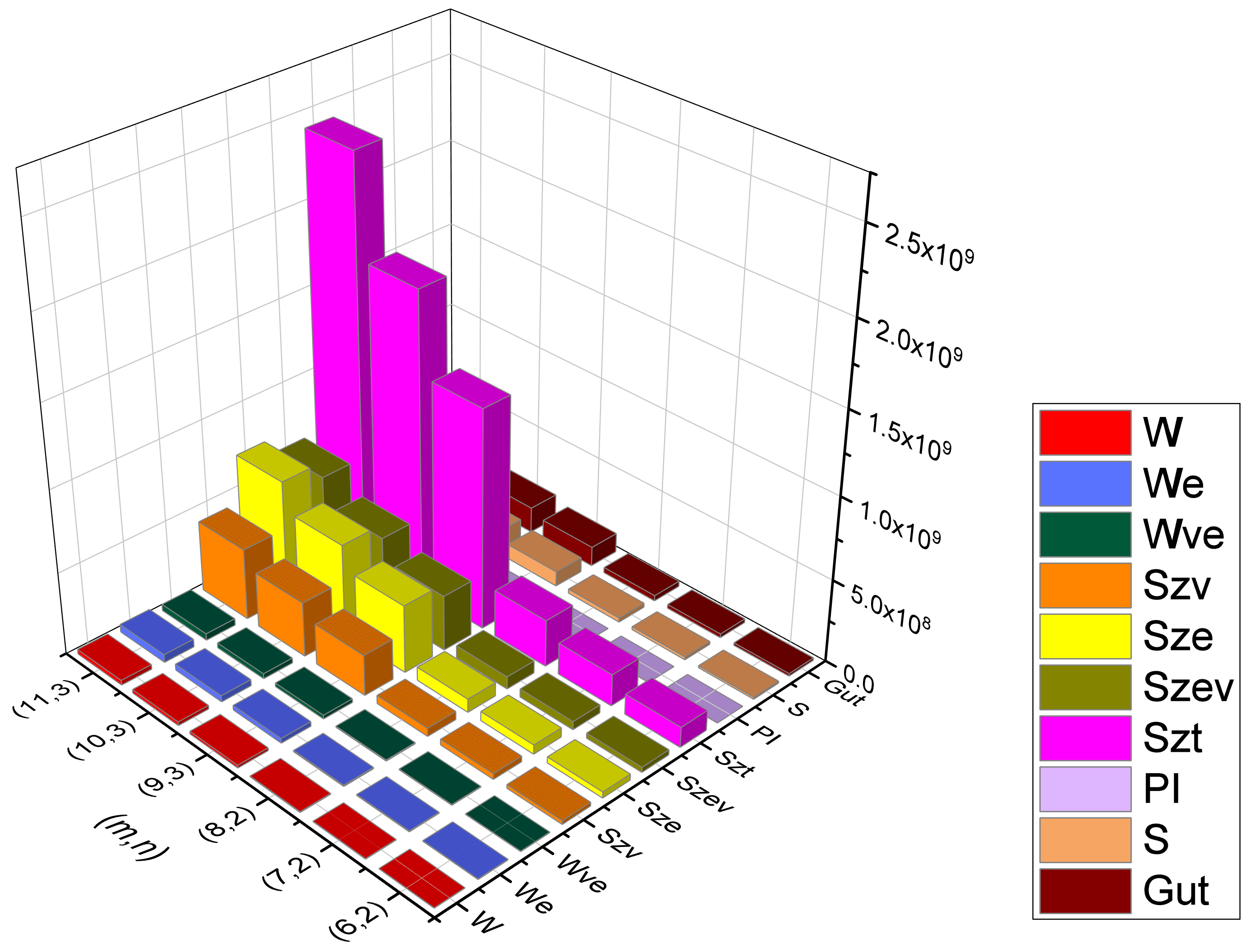
Figure 16.
Graphical representation of Type-II, .
Figure 16.
Graphical representation of Type-II, .
Table 1.
Type-I rectangular kekulene quotient graphs’ strength-weighted values, .
Table 1.
Type-I rectangular kekulene quotient graphs’ strength-weighted values, .
| QG | | |
|---|
|
|
|
|
|
|
|
|
|
|
|
|
|
|
|
|
|
|
|
|
|
|
|
|
|
|
|
|
|
|
|
|
|
|
|
|
|
|
|
|
|
|
Table 2.
Type-II rectangular kekulene quotient graphs’ strength-weighted values, .
Table 2.
Type-II rectangular kekulene quotient graphs’ strength-weighted values, .
| QG | | |
|---|
|
|
|
|
|
|
|
|
|
|
|
|
|
|
|
|
|
|
|
|
|
|
|
|
|
|
|
|
|
|
Table 3.
Numerical data for various topological indices of Type-I rectangular kekulene, .
Table 3.
Numerical data for various topological indices of Type-I rectangular kekulene, .
| TI | | | | | | |
|---|
| W | 1,529,326 | 12,892,583 | 56,651,252 | 176,719,457 | 445,629,018 | 971,766,315 |
| 2,441,352 | 21,357,446 | 95,542,356 | 301,219,250 | 764,945,248 | 1,676,476,958 |
| 1,932,744 | 16,595,584 | 73,574,892 | 230,728,252 | 583,866,944 | 1,276,405,096 |
| 14,122,936 | 178,900,160 | 1,049,163,296 | 4,093,341,864 | 12,391,103,016 | 31,532,413,808 |
| 22,602,448 | 296,922,164 | 1,771,941,688 | 6,984,978,108 | 21,289,569,952 | 54,441,498,564 |
| 17,870,172 | 230,496,884 | 1,363,540,172 | 5,347,312,020 | 16,242,326,140 | 41,433,430,836 |
| 72,465,728 | 936,816,092 | 5,548,185,328 | 21,772,944,012 | 66,165,325,248 | 168,840,774,044 |
| 261,520 | 1,461,944 | 4,817,200 | 12,030,552 | 25,302,928 | 47,332,920 |
| S | 7,935,312 | 67,508,352 | 297,984,656 | 932,079,328 | 2,354,695,504 | 5,141,520,960 |
| 10,293,184 | 88,370,384 | 391,844,240 | 1,229,017,952 | 3,110,525,856 | 6,800,795,568 |
Table 4.
Numerical data for various topological indices of Type-II rectangular kekulene, .
Table 4.
Numerical data for various topological indices of Type-II rectangular kekulene, .
| TI | | | | | | |
|---|
| W | 1,722,529 | 14,156,655 | 60,785,723 | 186,359,801 | 463,838,173 | 1,001,303,643 |
| 2,761,794 | 23,703,170 | 104,161,626 | 324,060,362 | 814,813,138 | 1,772,189,810 |
| 2,181,608 | 18,339,132 | 79,752,744 | 246,548,292 | 617,258,824 | 1,338,352,780 |
| 16,210,052 | 198,646,488 | 1,132,439,628 | 4,327,184,312 | 12,897,023,156 | 32,430,540,184 |
| 26,031,212 | 334,230,956 | 1,953,733,580 | 7,584,990,380 | 22,857,516,332 | 57,945,771,308 |
| 41,091,656 | 516,150,168 | 2,984,300,216 | 11,509,390,152 | 34,529,108,840 | 87,252,559,544 |
| 124,424,576 | 1,565,177,780 | 9,054,773,640 | 34,930,954,996 | 104,812,757,168 | 264,881,430,580 |
| 286,504 | 1,579,944 | 5,137,720 | 12,704,568 | 26,522,888 | 49,332,744 |
| S | 8,949,992 | 74,572,496 | 322,939,352 | 995,869,824 | 2,489,185,224 | 5,390,821,680 |
| 11,625,280 | 97,990,320 | 426,964,400 | 1,321,733,792 | 3,312,442,336 | 7,187,653,584 |
Table 5.
Numerical data for various topological indices of Type-I rectangular kekulene, .
Table 5.
Numerical data for various topological indices of Type-I rectangular kekulene, .
| TI | | | | | | |
|---|
| W | 2,382,825 | 3,509,404 | 4,948,263 | 17,307,562 | 22,640,917 | 28,982,536 |
| 3,840,674 | 5,699,828 | 8,086,526 | 28,793,524 | 37,803,722 | 48,544,840 |
| 3,163,474 | 4,832,900 | 7,005,422 | 23,012,176 | 30,916,824 | 40,457,928 |
| 22,992,284 | 34,960,304 | 50,491,572 | 247,647,280 | 332,059,920 | 433,745,600 |
| 37,104,636 | 56,790,072 | 82,453,956 | 412,500,280 | 554,800,556 | 726,607,952 |
| 31,416,480 | 50,319,732 | 75,393,800 | 336,115,552 | 469,051,260 | 632,132,168 |
| 122,929,880 | 192,389,840 | 283,733,128 | 1,332,378,664 | 1,824,962,996 | 2,424,617,888 |
| 363,720 | 482,800 | 618,760 | 1,819,248 | 2,215,672 | 2,651,216 |
| S | 12,386,344 | 18,267,792 | 25,785,736 | 90,702,304 | 118,735,472 | 152,082,736 |
| 16,096,080 | 23,772,112 | 33,592,128 | 118,832,080 | 155,668,576 | 199,507,072 |
Table 6.
Numerical data for various topological indices of Type-II rectangular kekulene, .
Table 6.
Numerical data for various topological indices of Type-II rectangular kekulene, .
| TI | | | | | | |
|---|
| W | 2,643,044 | 3,846,719 | 5,372,754 | 18,846,722 | 24,482,893 | 31,155,056 |
| 4,275,428 | 6,266,558 | 8,802,896 | 31,661,632 | 41,247,974 | 52,618,996 |
| 3,511,224 | 5,296,216 | 7,600,984 | 25,190,464 | 33,579,148 | 43,653,584 |
| 25,849,432 | 38,707,996 | 55,250,320 | 271,762,600 | 360,917,096 | 467,700,696 |
| 41,831,848 | 63,024,532 | 90,404,464 | 458,729,552 | 610,907,812 | 793,550,696 |
| 65,777,296 | 98,796,088 | 141,363,616 | 707,258,416 | 940,568,808 | 1,220,296,896 |
| 199,235,872 | 299,324,704 | 428,382,016 | 2,145,008,984 | 2,852,962,524 | 3,701,845,184 |
| 393,104 | 516,584 | 656,944 | 1,950,656 | 2,360,488 | 2,809,440 |
| S | 13,754,496 | 20,042,792 | 28,020,960 | 99,313,648 | 129,050,688 | 164,258,496 |
| 17,894,240 | 26,106,992 | 36,534,384 | 130,568,400 | 169,736,320 | 216,121,280 |
Table 7.
Comparison of numerical data of
Type-I and Type-II rectangular kekulene defined in [
53].
Table 7.
Comparison of numerical data of
Type-I and Type-II rectangular kekulene defined in [
53].
| S. No. | Des | | | Old | | | Old |
|---|
| | | | | | | | |
| 1 | | 396 | 414 | 378 | 926 | 962 | 890 |
| 2 | | 516 | 540 | 492 | 1216 | 1264 | 1168 |
| 3 | W | 1,529,326 | 1,722,529 | 1,351,715 | 12,892,583 | 14,156,655 | 11,606,991 |
| 4 | | 2,441,352 | 2,761,794 | 2,147,798 | 21,357,446 | 23,703,170 | 19,178,010 |
| 5 | | 1,932,744 | 2,181,608 | 1,704,356 | 16,595,584 | 18,339,132 | 14,921,548 |
| 6 | | 14,122,936 | 16,210,052 | 12,220,444 | 178,900,160 | 198,646,488 | 158,477,928 |
| 7 | | 22,602,448 | 26,031,212 | 19,484,452 | 296,922,164 | 334,230,956 | 262,471,644 |
| 8 | | 17,870,172 | 4,1091,656 | 15,732,036 | 230,496,884 | 516,150,168 | 212,184,156 |
| 9 | | 72,465,728 | 124,424,576 | 63,168,968 | 936,816,092 | 1,565,177,780 | 845,317,884 |
| 10 | | 261,520 | 286,504 | 253,032 | 1,461,944 | 1,579,944 | 1,445,120 |
| 11 | S | 7,935,312 | 8,949,992 | 7,003,400 | 67,508,352 | 74,572,496 | 60,725,712 |
| 12 | | 10,293,184 | 11,625,280 | 907,0928 | 88,370,384 | 97,990,320 | 79,424,784 |


 ,
, 


