
The Lyotropic Nature of Halates: An Experimental Study
 ,
,  ,
,  , and
, and 
Abstract
1. Introduction
2. Results and Discussion
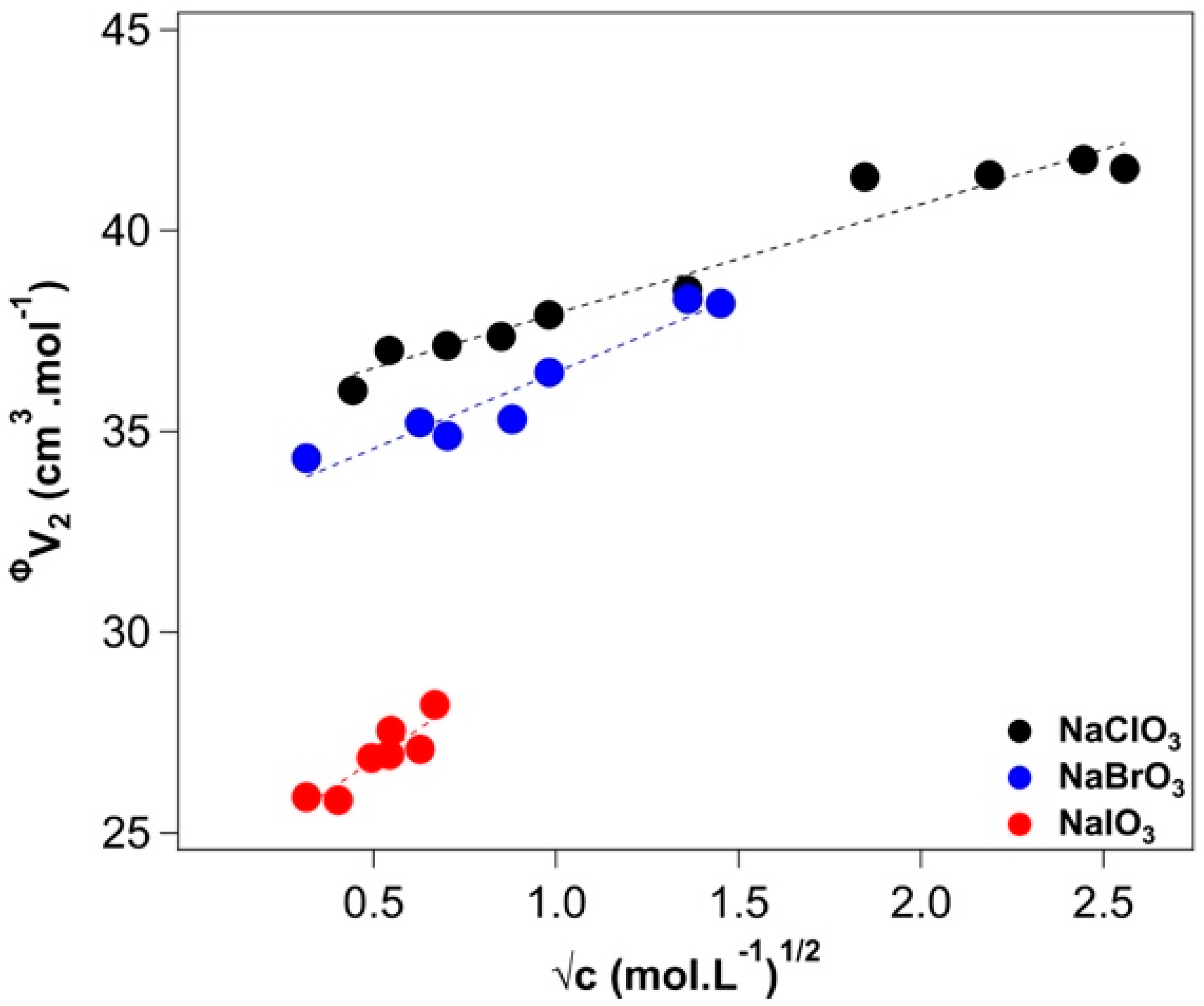
2.1. Density
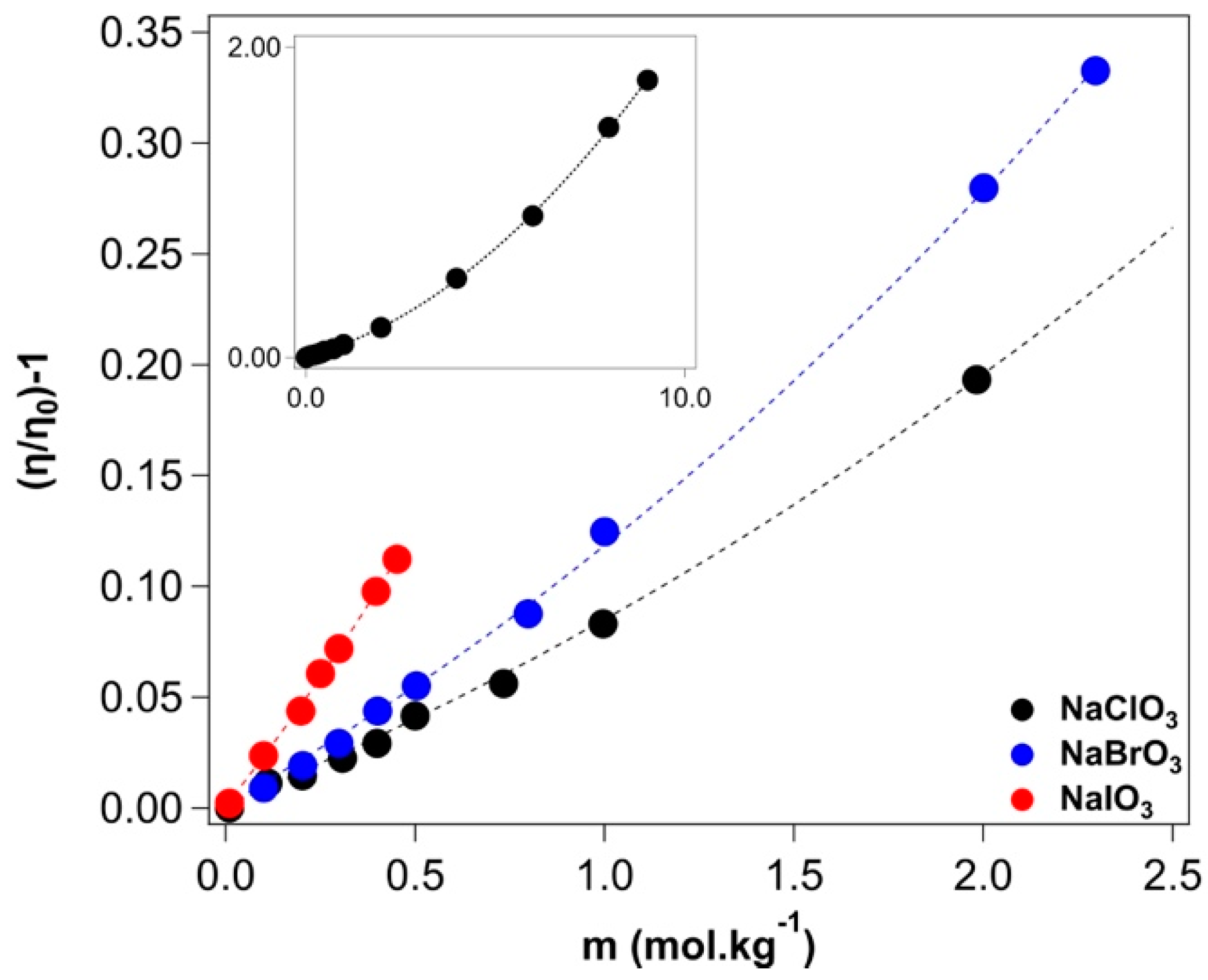
2.2. Viscosity
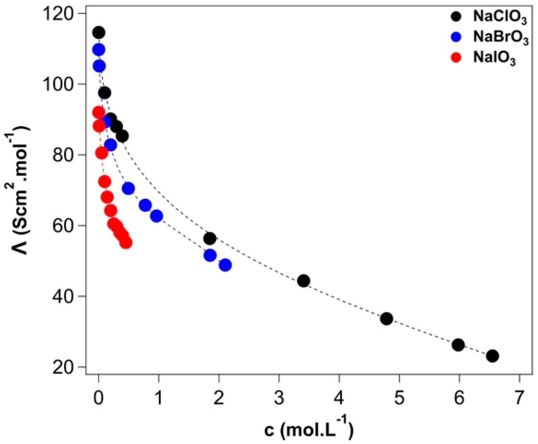
2.3. Conductivity
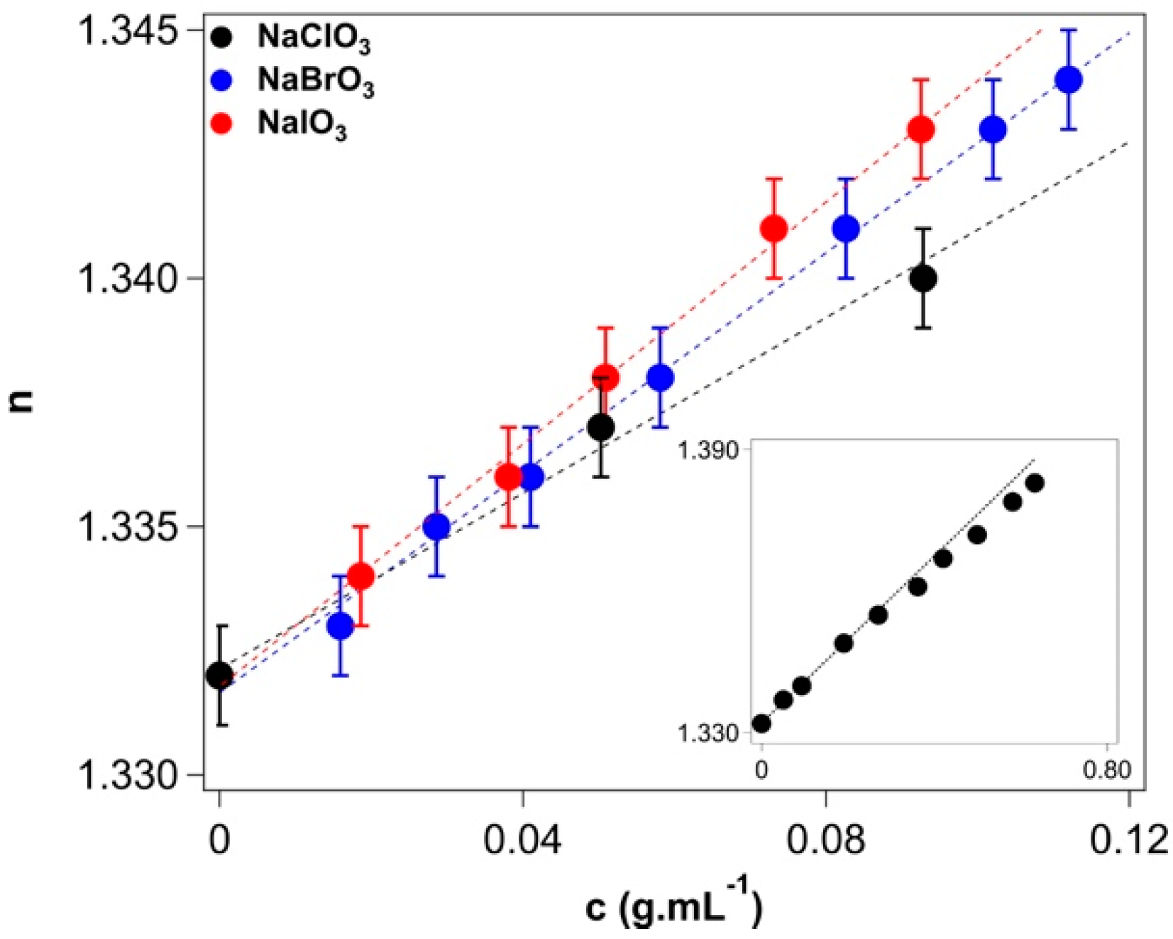
2.4. Refractive Index and Polarizability
2.5. Results from Previous Molecular Dynamics Studies
3. Materials and Methods
4. Conclusions
Supplementary Materials
Author Contributions
Funding
Institutional Review Board Statement
Informed Consent Statement
Data Availability Statement
Acknowledgments
Conflicts of Interest
Sample Availability
Appendix A
Appendix A.1. Density
>Appendix A.2. Viscosity
>Appendix A.3. Conductivity
>Appendix A.4. Refractive Index
References
- Gregory, K.P.; Elliott, G.R.; Robertson, H.; Kumar, A.; Wanless, E.J.; Webber, G.B.; Craig, V.S.J.; Andersson, G.G.; Page, A.J. Understanding Specific Ion Effects and the Hofmeister Series. Phys. Chem. Chem. Phys. 2022, 24, 12682–12718. [Google Scholar] [CrossRef] [PubMed]
- Salis, A.; Ninham, B.W. Models and Mechanisms of Hofmeister Effects in Electrolyte Solutions, and Colloid and Protein Systems Revisited. Chem. Soc. Rev. 2014, 43, 7358–7377. [Google Scholar] [CrossRef] [PubMed]
- Bruce, E.E.; Okur, H.I.; Stegmaier, S.; Drexler, C.I.; Rogers, B.A.; van der Vegt, N.F.A.; Roke, S.; Cremer, P.S. Molecular Mechanism for the Interactions of Hofmeister Cations with Macromolecules in Aqueous Solution. J. Am. Chem. Soc. 2020, 142, 19094–19100. [Google Scholar] [CrossRef] [PubMed]
- Schwierz, N.; Horinek, D.; Netz, R.R. Anionic and Cationic Hofmeister Effects on Hydrophobic and Hydrophilic Surfaces. Langmuir 2013, 29, 2602–2614. [Google Scholar] [CrossRef] [PubMed]
- Ninham, B.W.; Yaminsky, V. Ion Binding and Ion Specificity: The Hofmeister Effect and Onsager and Lifshitz Theories. Langmuir 1997, 13, 2097–2108. [Google Scholar] [CrossRef]
- Yaminsky, V.V.; Ninham, B.W. Hydrophobic force: Lateral enhancement of subcritical fluctuations. Langmuir 1993, 9, 3618–3624. [Google Scholar] [CrossRef]
- Tatini, D.; Ciardi, D.; Sofroniou, C.; Ninham, B.W.; Lo Nostro, P. Physicochemical Characterization of Green Sodium Oleate-Based Formulations. Part 2. Effect of Anions. J. Colloid Interface Sci. 2022, 617, 399–408. [Google Scholar] [CrossRef]
- Budroni, M.A.; Rossi, F.; Marchettini, N.; Wodlei, F.; Lo Nostro, P.; Rustici, M. Hofmeister Effect in Self-Organized Chemical Systems. J. Phys. Chem. B 2020, 124, 9658–9667. [Google Scholar] [CrossRef]
- Lo Nostro, P.; Ninham, B.W. Hofmeister Phenomena: An Update on Ion Specificity in Biology. Chem. Rev. 2012, 112, 2286–2322. [Google Scholar] [CrossRef]
- Mazzini, V.; Craig, V.S.J. Volcano Plots Emerge from a Sea of Nonaqueous Solvents: The Law of Matching Water Affinities Extends to All Solvents. ACS Cent. Sci. 2018, 4, 1056–1064. [Google Scholar] [CrossRef]
- Lo Nostro, P.; Lo Nostro, A.; Ninham, B.W.; Pesavento, G.; Fratoni, L.; Baglioni, P. Hofmeister Specific Ion Effects in Two Biological Systems. Curr. Opin. Colloid Interface Sci. 2004, 9, 97–101. [Google Scholar] [CrossRef]
- Lonetti, B.; Lo Nostro, P.; Ninham, B.W.; Baglioni, P. Anion Effects on Calixarene Monolayers: A Hofmeister Series Study. Langmuir 2005, 21, 2242–2249. [Google Scholar] [CrossRef]
- Salis, A.; Pinna, M.C.; Bilaničová, D.; Monduzzi, M.; Lo Nostro, P.; Ninham, B.W. Specific Anion Effects on Glass Electrode pH Measurements of Buffer Solutions: Bulk and Surface Phenomena. J. Phys. Chem. B 2006, 110, 2949–2956. [Google Scholar] [CrossRef] [PubMed]
- Lagi, M.; Lo Nostro, P.; Fratini, E.; Ninham, B.W.; Baglioni, P. Insights into Hofmeister Mechanisms: Anion and Degassing Effects on the Cloud Point of Dioctanoylphosphatidylcholine/Water Systems. J. Phys. Chem. B 2007, 111, 589–597. [Google Scholar] [CrossRef] [PubMed]
- Pyper, N.C.; Pike, C.G.; Edwards, P.P. The Polarizabilities of Species Present in Ionic Solutions. Mol. Phys. 1992, 76, 353–372. [Google Scholar] [CrossRef]
- Marcus, Y. Individual Ionic Surface Tension Increments in Aqueous Solutions. Langmuir 2013, 29, 2881–2888. [Google Scholar] [CrossRef]
- Voet, A. Quantative Lyotropy. Chem. Rev. 1937, 20, 169–179. [Google Scholar] [CrossRef]
- Marcus, Y. Thermodynamics of solvation of ions. Part 5.—Gibbs free energy of hydration at 298.15 K. J. Chem. Soc. Faraday Trans. 1991, 87, 2995–2999. [Google Scholar] [CrossRef]
- Marcus, Y. The Hydration Entropies of Ions and Their Effects on the Structure of Water. J. Chem. Soc. Faraday Trans. 1986, 82, 233–242. [Google Scholar] [CrossRef]
- Krestov, G.A. Thermodynamics of Solvation: Solution and Dissolution, Ions and Solvents, Structure and Energetics; Ellis Horwood: New York, NY, USA, 1991. [Google Scholar]
- Jenkins, H.D.B.; Marcus, Y. Viscosity B-coefficients of ions in solution. Chem. Rev. 1995, 95, 2695–2724. [Google Scholar] [CrossRef]
- Collins, K.D.; Washabaugh, M.W. The Hofmeister Effect and the Behaviour of Water at Interfaces. Q. Rev. Biophys. 1985, 18, 323–422. [Google Scholar] [CrossRef]
- Mazzini, V.; Craig, V.S.J. Specific-Ion Effects in Non-Aqueous Systems. Curr. Opin. Colloid Interface Sci. 2016, 23, 82–93. [Google Scholar] [CrossRef]
- Sarri, F.; Tatini, D.; Tanini, D.; Simonelli, M.; Ambrosi, M.; Ninham, B.W.; Capperucci, A.; Dei, L.; Lo Nostro, P. Specific Ion Effects in Non-Aqueous Solvents: The Case of Glycerol Carbonate. J. Mol. Liq. 2018, 266, 711–717. [Google Scholar] [CrossRef]
- Timson, D.J. The roles and applications of chaotropes and kosmotropes in industrial fermentation processes. World J. Microbiol. Biotechnol. 2020, 36, 89. [Google Scholar] [CrossRef]
- Marcus, Y. Effect of Ions on the Structure of Water: Structure Making and Breaking. Chem. Rev. 2009, 109, 1346–1370. [Google Scholar] [CrossRef]
- Edelman, R.; Kusner, I.; Kisiliak, R.; Srebnik, S.; Livney, Y.D. Sugar stereochemistry effects on water structure and on protein stability: The templating concept. Food Hydrocoll. 2015, 48, 27–37. [Google Scholar] [CrossRef]
- Leontidis, E. Chaotropic salts interacting with soft matter: Beyond the lyotropic series. Curr. Op. Coll. Interface Sci. 2016, 23, 100–109. [Google Scholar] [CrossRef]
- Zangi, R. Can salting-in/salting-out ions be classified as chaotropes/kosmotropes? J. Phys. Chem. B 2010, 114, 643–650. [Google Scholar] [CrossRef]
- Zhang, Y.; Furyk, S.; Sagle, L.B.; Cho, Y.; Bergbreiter, D.E.; Cremer, D.E. Effects of Hofmeister Anions on the LCST of PNIPAM as a Function of Molecular Weight. J. Phys. Chem. C 2007, 111, 8916–8924. [Google Scholar] [CrossRef]
- Mittal, N.; Benselfelt, T.; Ansari, F.; Gordeyeva, K.; Roth, S.V.; Wågberg, L.; Söderberg, L.D. Ion-Specific Assembly of Strong, Tough, and Stiff Biofibers. Angew. Chem. Int. Ed. 2019, 58, 18562–18569. [Google Scholar] [CrossRef]
- Cray, J.A.; Russell, J.T.; Timson, D.J.; Singhal, R.S.; Hallsworth, J.E. A universal measure of chaotropicity and kosmotropicity. Environ. Microbiol. 2013, 15, 287–296. [Google Scholar] [CrossRef] [PubMed]
- Gibb, B.C. Abiogenesis and the reverse Hofmeister effect. Nat. Chem. 2018, 10, 797–798. [Google Scholar] [CrossRef] [PubMed]
- Cockell, C.S.; McLean, C.M.; Perera, L.; Aka, S.; Stevens, A.; Dickinson, A.W. Growth of Non-Halophilic Bacteria in the Sodium-Magnesium-Sulfate-Chloride Ion System: Unravelling the Complexities of Ion Interactions in Terrestrial and Extraterrestrial Aqueous Environments. Astrobiology 2020, 20, 944–955. [Google Scholar] [CrossRef] [PubMed]
- Heinz, J.; Rambags, V.; Schulze-Makuch, D. Physicochemical Parameters Limiting Growth of Debaryomyces hansenii in Solutions of Hygroscopic Compounds and Their Effects on the Habitability of Martian Brines. Life 2021, 11, 1194. [Google Scholar] [CrossRef]
- Ball, P.; Hallsworth, J.E. Water structure and chaotropicity: Their uses, abuses and biological implications. Phys. Chem. Chem. Phys. 2015, 17, 8297–8305. [Google Scholar] [CrossRef]
- Dos Santos, A.P.; Diehl, A.; Levin, Y. Surface Tensions, Surface Potentials, and the Hofmeister Series of Electrolyte Solutions. Langmuir 2010, 26, 10778–10783. [Google Scholar] [CrossRef] [PubMed]
- Baer, M.D.; Pham, V.T.; Fulton, J.L.; Schenter, G.K.; Balasubramanian, M.; Mundy, C.J. Is Iodate a Strongly Hydrated Cation? J. Phys. Chem. Lett. 2011, 2, 2650–2654. [Google Scholar] [CrossRef]
- Sharma, B.; Chandra, A. Born–Oppenheimer Molecular Dynamics Simulations of a Bromate Ion in Water Reveal Its Dual Kosmotropic and Chaotropic Behavior. J. Phys. Chem. B 2018, 122, 2090–2101. [Google Scholar] [CrossRef]
- Millero, F.J. Molal volumes of electrolytes. Chem. Rev. 1971, 71, 147–176. [Google Scholar] [CrossRef]
- Collins, K.D. Ions from the Hofmeister series and osmolytes: Effects on proteins in solution and in the crystallization process. Methods 2004, 34, 300–311. [Google Scholar] [CrossRef]
- Collins, K.D. The behavior of ions in water is controlled by their water affinity. Q. Rev. Biophys. 2019, 52, E11. [Google Scholar] [CrossRef] [PubMed]
- Padova, J. Solvation Approach to Ion Solvent Interaction. J. Chem. Phys. 1964, 40, 691–694. [Google Scholar] [CrossRef]
- Mazzini, V.; Craig, V.S.J. What is the fundamental ion-specific series for anions and cations? Ion specificity in standard partial molar volumes of electrolytes and electrostriction in water and non-aqueous solvents. Chem. Sci. 2017, 8, 7052–7065. [Google Scholar] [CrossRef] [PubMed]
- Harned, H.S.; Owen, B.B.; King, C. The Physical Chemistry of Electrolytic Solutions; Reinhold Publishing Corporation: New York, NY, USA, 1943. [Google Scholar]
- Falkenhagen, H.; Vernon, E. The quantitative limiting law for the viscosity of simple strong electrolytes. Physik. Z. 1932, 33, 140. [Google Scholar]
- Schwierz, N.; Horinek, D.; Sivan, U.; Netz, R.R. Reversed Hofmeister series—The rule rather than the exception. Curr. Opin. Colloid Interface Sci. 2016, 23, 10–18. [Google Scholar] [CrossRef]
- Collins, K.D. Charge Density-Dependent Strength of Hydration and Biological Structure. Biophys. J. 1997, 72, 65–76. [Google Scholar] [CrossRef] [PubMed]
- Haynes, W.M.; Lide, D.R.; Bruno, T.J. CRC Handbook of Chemistry and Physics; CRC press: Boca Raton, FL, USA, 2016. [Google Scholar]
- Eysel, H.H.; Lipponer, K.G.; Oberle, C.; Zahn, I. Raman intensities of liquids: Absolute scattering activities and electro-optical parameters of the halate ions ClO3−, BrO3−, and IO3− in aqueous solutions. Spectrochim. Acta Part Mol. Spectrosc. 1992, 48, 219–224. [Google Scholar] [CrossRef]
- Li, M.; Zhuang, B.; Lu, Y.; Wang, Z.G.; An, L. Accurate Determination of Ion Polarizabilities in Aqueous Solutions. J. Phys. Chem. B 2017, 121, 6416–6424. [Google Scholar] [CrossRef]
- Oberle, C.; Eysel, H.H. Ab initio calculations for some oxo-anions of chlorine, bromine and iodine. J. Mol. Struct. THEOCHEM 1993, 280, 107–115. [Google Scholar] [CrossRef]
- Rabek, J.F. Experimental Methods in Polymer Chemistry: Physical Principles and Applications; John Wiley & Sons Ltd.: Hoboken, NJ, USA, 1991. [Google Scholar]
- Robinson, R.A.; Stokes, R.H. Tables of osmotic and activity coefficients of electrolytes in aqueous solution at 25 °C. Trans. Faraday Soc. 1949, 45, 612–624. [Google Scholar] [CrossRef]
- Durig, J.R.; Bonner, O.; Breazeale, W. Raman studies of iodic acid and sodium iodate. J. Phys. Chem. 1965, 69, 3886–3892. [Google Scholar] [CrossRef]
- Marcus, Y. Electrostriction in electrolyte solutions. Chem. Rev. 2011, 111, 2761–2783. [Google Scholar] [CrossRef] [PubMed]
- Marcus, Y.; Hefter, G. Standard partial molar volumes of electrolytes and ions in nonaqueous solvents. Chem. Rev. 2004, 104, 3405–3452. [Google Scholar] [CrossRef] [PubMed]
- Hamann, S.; Lim, S. The volume change on ionization of weak electrolytes. Aust. J. Chem. 1954, 7, 329–334. [Google Scholar] [CrossRef]
- Lo Nostro, P.; Ninham, B.W.; Milani, S.; Lo Nostro, A.; Pesavento, G.; Baglioni, P. Hofmeister effects in supramolecular and biological systems. Biophys. Chem. 2006, 124, 208–213. [Google Scholar] [CrossRef] [PubMed]
- Parsons, D.F.; Boström, M.; Lo Nostro, P.; Ninham, B.W. Hofmeister effects: Interplay of hydration, nonelectrostatic potentials, and ion size. Phys. Chem. Chem. Phys. 2011, 13, 12352–12367. [Google Scholar] [CrossRef]
- Lewis, G.N.; Randall, M.; Pitzer, K.S.; Brewer, L. Thermodynamics; Courier Dover Publications: Mineola, NY, USA, 2020. [Google Scholar]
- Millero, F.J. The apparent and partial molal volume of aqueous sodium chloride solutions at various temperatures. J. Phys. Chem. 1970, 74, 356–362. [Google Scholar] [CrossRef]
- Roy, M.N.; De, P.; Sikdar, P.S. Physicochemical study of solution behaviour of alkali metal perchlorates prevailing in N,N-Dimethyl Formamide with the manifestation of ion solvation consequences. J. Mol. Liq. 2015, 204, 243–247. [Google Scholar] [CrossRef]
- Tomaš, R.; Kinart, Z.; Tot, A.; Papović, S.; Teodora Borović, T.; Vraneš, M. Volumetric properties, conductivity and computation analysis of selected imidazolium chloride ionic liquids in ethylene glycol. J. Mol. Liq. 2022, 345, 118178. [Google Scholar] [CrossRef]
- Shekaari, H.; Jebali, F. Densities, Viscosities, Electrical Conductances, and Refractive Indices of Amino Acid + Ionic Liquid ([BMIm]Br) + Water Mixtures at 298.15 K. J. Chem. Eng. Data 2010, 55, 2517–2523. [Google Scholar] [CrossRef]
- Marcus, Y. On the intrinsic volumes of ions in aqueous solutions. J. Sol. Chem. 2010, 39, 1031–1038. [Google Scholar] [CrossRef]
- Pedersen, T.G.; Dethlefsen, C.; Hvidt, A. Volumetric properties of aqueous solutions of alkali halides. Carlsberg Res. Commun. 1984, 49, 445–455. [Google Scholar] [CrossRef]
- Cox, W.; Wolfenden, J. The viscosity of strong electrolytes measured by a differential method. Proc. Roy. Soc. A 1934, 145, 475–488. [Google Scholar] [CrossRef]
- Jones, G.; Dole, M. The viscosity of aqueous solutions of strong electrolytes with special reference to barium chloride. J. Am. Chem. Soc. 1929, 51, 2950–2964. [Google Scholar] [CrossRef]
- Jiang, J.; Sandler, S.I. A New Model for the Viscosity of Electrolyte Solutions. Ind. Eng. Chem. Res. 2003, 42, 6267–6272. [Google Scholar] [CrossRef]
- Horvath, A.L.; Horwood, E. Handbook of Aqueous Electrolyte Solutions; Halsted Press: Sydney, Australia, 1985. [Google Scholar]
- Patil, R.S.; Shaikh, V.R.; Patil, P.D.; Borse, A.U.; Patil, K.J. The viscosity B and D coefficient (Jones–Dole equation) studies in aqueous solutions of alkyltrimethylammonium bromides at 298.15 K. J. Mol. Liq. 2014, 200, 416–424. [Google Scholar] [CrossRef]
- Mitchell, D.J.; Ninham, B.W. Range of the Screened Coulomb Interaction in Electrolytes and Double Layer Problems. Chem. Phys. Lett. 1978, 53, 397–399. [Google Scholar] [CrossRef]
- Kékicheff, P.; Ninham, B.W. The Double-Layer Interaction in Asymmetric Electrolytes. EPL 1990, 12, 471–477. [Google Scholar] [CrossRef]
- Nylander, T.; Kékicheff, P.; Ninham, B.W. The Effect of Solution Behavior of Insulin on Interactions between Adsorbed Layers of Insulin. J. Colloid Interface Sci. 1994, 164, 136–150. [Google Scholar] [CrossRef]
- Robinson, R.A.; Stokes, R.H. Electrolyte Solutions; Butterworths Scientific Publications: London, UK, 1959. [Google Scholar]
- Poiseuille, J.L.M. Experimental investigations on the flow of liquids in tubes of very small diameter. Ann. Chim. Phys. 1847, 21, 76. [Google Scholar]
- Partington, J.R. A History of Chemistry; Martino Fine Books: Eastford, CT, USA, 1961; Volume 3. [Google Scholar]
- Tamamushi, R. Estimation of Individual Ionic Activity Coefficients from Conductivity Data on Strong Electrolytes in Dilute Aqueous Solutions. Bull. Chem. Soc. Jpn. 1974, 47, 1921–1926. [Google Scholar] [CrossRef]
- Tamamushi, R. A Method for Determining the Degree of Dissociation of Symmetrical Associated Electrolytes from the Conductivity and Activity Data. Bull. Chem. Soc. Jpn. 1975, 48, 705–706. [Google Scholar] [CrossRef]
- Onsager, L.; Fuoss, R.M. Irreversible Processes in Electrolytes. Diffusion, Conductance and Viscous Flow in Arbitrary Mixtures of Strong Electrolytes. J. Phys. Chem. 1932, 36, 2689–2778. [Google Scholar] [CrossRef]
- Fuoss, R.M.; Hsia, K.L. Association of 1-1 salts in water. Proc. Natl. Acad. Sci. USA 1967, 57, 1550–1557. [Google Scholar] [CrossRef]
- Fernandez-Prini, R.; Justice, J.C. Evaluation of the solubility of electrolytes from conductivity measurements. Pure Appl. Chem. 1984, 56, 541–547. [Google Scholar] [CrossRef]
- Williams, J.W.; Falkenhagen, H. The Interionic Attraction Theory of Electrical Conductance. Chem. Rev. 1929, 6, 317–345. [Google Scholar] [CrossRef]
- Ninham, B.W.; Lo Nostro, P. Molecular Forces and Self Assembly: In Colloid, Nano Sciences and Biology; Cambridge University Press: Cambridge, UK, 2010. [Google Scholar]
- Marcus, Y. Ionic radii in aqueous solution. Chem. Rev. 1988, 88, 1475–1498. [Google Scholar] [CrossRef]
- De Feijter, J.A.; Benjamins, J.; Veer, F.A. Ellipsometry as a tool to study the adsorption behavior of synthetic and biopolymers at the air–water interface. Biopolym. Orig. Res. Biomol. 1978, 17, 1759–1772. [Google Scholar] [CrossRef]
- Ball, V. Hofmeister Effects of Monovalent Sodium Salts in the Gelation Kinetics of Gelatin. J. Phys. Chem. B 2019, 123, 8405–8410. [Google Scholar] [CrossRef]
- Born, M.; Wolf, E. Principles of optics: Electromagnetic theory of propagation, interference and diffraction of light; Cambridge University Press: Cambridge, UK, 1999. [Google Scholar]


| Salt | [40] | ||||
|---|---|---|---|---|---|
| NaClO3 | 35.7 ± 0.2 | 35.5 | −9.4 ± 0.2 | −21 | 2.7 ± 0.2 |
| NaBrO3 | 32.8 ± 0.2 | 34.1 | −14.4 ± 0.2 | −31 | 3.8 ± 0.5 |
| NaIO3 | 24.7 ± 0.3 | 24.1 | −12.1 ± 0.3 | −33 | 6.2 ± 1.3 |
| Halate | A | BJD | D | Halide | BJD | |
|---|---|---|---|---|---|---|
| This Work | Ref. [21] | Ref. [21] | ||||
| NaClO3 | 0.0066 | 0.064 ± 0.002 | 0.063 | 0.015 ± 0.001 | NaCl | 0.080 |
| NaBrO3 | 0.0071 | 0.089 ± 0.004 | 0.094 | 0.023 ± 0.002 | NaBr | 0.052 |
| NaIO3 | 0.0083 | 0.197 ± 0.008 | 0.225 | 0.089 ± 0.021 | NaI | 0.012 |
| Salt | This Work | Ref. [49] |
|---|---|---|
| NaClO3 | 116.51 ± 0.74 | 114.68 |
| NaBrO3 | 112.22 ± 0.36 | 105.78 |
| NaIO3 | 91.98 ± 0.98 | 90.58 |
| Salt | nsalt | α | A a |
|---|---|---|---|
| NaClO3 | 1.553 ± 0.007 | 5.40 ± 0.06 | 5.23 (5.43) |
| NaBrO3 | 1.702 ± 0.007 | 6.94 ± 0.05 | 6.47 (6.49) |
| NaIO3 | 1.854 ± 0.009 | 8.22 ± 0.07 | 8.01 (7.64) |
| Ion | ra | Δr a | na | ΔhydrG a | ΔhydrS b | Nc | k1 d | ΔSII e |
|---|---|---|---|---|---|---|---|---|
| Na+ | 0.102 | 0.116 | 3.5 | −365 | −111 | 100 | 1.20 | −5.4 |
| ClO3− | 0.200 | 0.033 | 1.8 | −280 | −80 | 10.65 | 0.00 | 5.0 |
| BrO3− | 0.191 | 0.038 | 1.9 | −330 | −95 | 9.55 | 0.35 | −5.0 |
| IO3− | 0.181 | 0.043 | 2.0 | −400 | −148 | 6.25 | 0.70 | (−47) |
Publisher’s Note: MDPI stays neutral with regard to jurisdictional claims in published maps and institutional affiliations. |
© 2022 by the authors. Licensee MDPI, Basel, Switzerland. This article is an open access article distributed under the terms and conditions of the Creative Commons Attribution (CC BY) license (https://creativecommons.org/licenses/by/4.0/).
Share and Cite
Acar, M.; Tatini, D.; Ninham, B.W.; Rossi, F.; Marchettini, N.; Lo Nostro, P. The Lyotropic Nature of Halates: An Experimental Study. Molecules 2022, 27, 8519. https://doi.org/10.3390/molecules27238519
Acar M, Tatini D, Ninham BW, Rossi F, Marchettini N, Lo Nostro P. The Lyotropic Nature of Halates: An Experimental Study. Molecules. 2022; 27(23):8519. https://doi.org/10.3390/molecules27238519
Chicago/Turabian StyleAcar, Mert, Duccio Tatini, Barry W. Ninham, Federico Rossi, Nadia Marchettini, and Pierandrea Lo Nostro. 2022. "The Lyotropic Nature of Halates: An Experimental Study" Molecules 27, no. 23: 8519. https://doi.org/10.3390/molecules27238519
APA StyleAcar, M., Tatini, D., Ninham, B. W., Rossi, F., Marchettini, N., & Lo Nostro, P. (2022). The Lyotropic Nature of Halates: An Experimental Study. Molecules, 27(23), 8519. https://doi.org/10.3390/molecules27238519