Article

Predictive Models of Gas/Particulate Partition Coefficients (KP) for Polycyclic Aromatic Hydrocarbons and Their Oxygen/Nitrogen Derivatives

College of Geography and Environmental Sciences, Zhejiang Normal University, Yingbin Avenue 688, Jinhua 321004, China
*
Author to whom correspondence should be addressed.
Molecules 2022, 27(21), 7608; https://doi.org/10.3390/molecules27217608
Submission received: 23 September 2022 / Revised: 3 November 2022 / Accepted: 3 November 2022 / Published: 6 November 2022

Abstract

:
Polycyclic aromatic hydrocarbons (PAHs) and their oxygen/nitrogen derivatives released into the atmosphere can alternate between a gas phase and a particulate phase, further affecting their environmental behavior and fate. The gas/particulate partition coefficient (KP) is generally used to characterize such partitioning equilibrium. In this study, the correlation between log KP of fifty PAH derivatives and their n-octanol/air partition coefficient (log KOA) was first analyzed, yielding a strong linear correlation (R2 = 0.801). Then, Gaussian 09 software was used to calculate quantum chemical descriptors of all chemicals at M062X/6-311+G (d,p) level. Both stepwise multiple linear regression (MLR) and support vector machine (SVM) methods were used to develop the quantitative structure-property relationship (QSPR) prediction models of log KP. They yield better statistical performance (R2 > 0.847, RMSE < 0.584) than the log KOA model. Simulation external validation and cross validation were further used to characterize the fitting performance, predictive ability, and robustness of the models. The mechanism analysis shows intermolecular dispersion interaction and hydrogen bonding as the main factors to dominate the distribution of PAH derivatives between the gas phase and particulate phase. The developed models can be used to predict log KP values of other PAH derivatives in the application domain, providing basic data for their ecological risk assessment.

1. Introduction

Polycyclic aromatic hydrocarbons (PAHs) are typical persistent organic pollutants (POPs) that are widely found in the environment [1]. Exposure to PAHs may lead to atherosclerosis, hypertension and myocardial infarction, and increase the risk of skin, lung, pancreas, stomach, intestinal and other cancers [2,3,4,5,6]. PAHs can further undergo photochemical reactions or be oxidized by atmospheric oxidants, such as O3, OH radicals and NOx, to generate oxygen/nitrogen derivatives, including oxidized PAHs (O-PAHs), nitro PAHs (N-PAHs) and azaarenes (AZAs) [7,8,9]. In addition, the incomplete combustion of fuels during human activities, vehicle and ship exhaust emissions, and industrial waste emissions also lead to the generation of PAHs and their oxygen/nitrogen derivatives [10,11,12,13]. In recent years, PAHs and their oxygen/nitrogen derivatives have been detected not only in the atmosphere, but also in soil, water, sediment and other environmental media and organisms [14,15,16,17,18]. Minero et al. [19] detected N-PAHs in atmospheric particles of Antarctica in the year 2010, indicating the global presence of PAH derivatives. PAH derivatives are generally trace compounds with concentrations of about one-tenth or even one-hundredth of the parent level in environmental media [20,21]. However, most PAH derivatives are direct mutagens or potential carcinogens [22], and some N-PAHs are even 10 times more carcinogenic or 100,000 times more mutagenic than their parent compounds [23,24,25], bringing high risk to human health and arousing widespread concern.
When PAHs and oxygen/nitrogen derivatives are released into the atmosphere from various sources, they can partly exist in gaseous form or partly combine with atmospheric particles to migrate over long distances, and finally move to the ground surface through atmospheric deposition [26]. Studying the distribution of these compounds between the atmosphere and particulate matter has great implications for understanding their environmental behavior and fate. The gas/particulate partition coefficient, KP, is often used to characterize such distribution equilibrium of organic pollutants and calculated by [27].
K P = C P C A   ×   TSP
Here, CP represents the concentration of organic matter in the atmospheric particle phase and CA represents the concentration in the air phase, with the unit of ng/m3; TSP refers to the concentration of total suspended particulate matter, in μg/m3.
Determining the KP values is time-consuming, laborious, and limited by standard samples of target compounds. Therefore, establishing a predictive model for KP can provide an important method to study the gas/particulate distribution behavior of pollutants and supply basic data for their ecological environment safety and health risk assessment.
Previous studies have shown that the n-octanol/air partition coefficient (KOA) can predict the KP values of organic pollutants such as PAHs, polychlorinated biphenyls (PCBs), polychlorinated naphthalenes (PCNs), and DDT [28,29]. However, the low prediction accuracy and the lack of KOA values for some compounds restricts the application of this method. A quantitative structure-property relationship (QSPR) model can be used to establish a quantitative relationship between compound properties, environmental behavior parameters and molecular structure feature through mathematical methods, and can further predict the properties and environmental behavior of similar compounds which lack experimental data [30,31,32,33,34].
Therefore, the goals of this study are first to analyze the correlation between log KP and log KOA of PAHs and oxygen/nitrogen derivatives, and then establish a QSPR prediction model for log KP by multiple linear regression (MLR) and support vector machine (SVM) methods. The model performance will be validated and evaluated, and the relevant mechanism and application domain will be discussed to further understand the partitioning process and predict more chemicals.

2. Materials and Methods

2.1. Log KP Experimental Values

In this study, the experimental CA, CP and TSP values of 50 PAHs and oxygen/nitrogen derivatives were obtained from the previous study [35], including 22 parent and alkyl PAHs, 15 O-PAHs, 9 N-PAHs and 4 AZAs. Then, the log KP value for every chemical is calculated by Equation (1). Information about all compounds as well as log KP data are listed in Table 1.

2.2. Descriptors

The intermolecular interactions, such as van der Waals forces (e.g., dispersion, dipole-dipole, dipole-induced dipole Interactions) and specific polarization (e.g., hydrogen bonding), are important factors to determine the distribution of organic chemicals between gas and particulate phases [36,37]. In this study, the molecular volume (V, cm3/mol), the dipole moment (d, Debye), the square of dipole moment (d2, Debye) and the average molecular polarization (α, a.u.) are selected to characterize dispersion, dipole–dipole and dipole-induced dipole interactions. The frontier molecular orbitals (ELUMO and EHOMO, eV), hardness (η, eV), softness (σ, eV), chemical potential (μ, eV) and electrophilic index (ω, eV) are used to quantify the ability of molecules to receive or provide electrons. Three charge descriptors, the most positive electrostatic charge of hydrogen atom (qH+, a.c.u.), the most positive electrostatic charge of carbon atom (qC+, a.c.u.) and the most negative electrostatic charge of carbon atom (qC, a.c.u.), are employed to characterize the charge information of the compounds. All 13 descriptors were obtained from the output files of molecular configuration optimization, which was carried out by using Gaussian 09 software [38] at M062X/6-311 + G (d, P) level. In addition, the parameters that characterize the electrostatic potential on the molecular surface are selected, including the most positive/negative electrostatic potential on the molecular surface (Vs.max/Vs.min, eV), the average value of the positive/negative electrostatic potential on the molecular surface ( V ¯ s + / V ¯ s , eV), the average dispersion of the electrostatic potential on the molecular surface (Π, eV), and the equilibrium constant of the electrostatic potential on the molecular surface (τ). These parameters were further calculated by GsGrid (Verison 1.7) software [39] based on the Gaussian output files. Moreover, the log KOA values of the compounds were calculated using EPI SuiteTM v4.11 software [40].

2.3. Model Construction and Verification

The stepwise regression method in IBM SPSS 21.0 software [41] was used to screen variables and build the MLR model. The regression performance, predictive capability and robustness of the model was assessed according to the OECD guidelines [42], the square of the correlation coefficient (R2), the square of the prediction correlation coefficient (Q2), the root-mean-square error (RMSE), the mean absolute error (MAE), the maximum positive error (MPE), the maximum negative error (MNE), and the systematic error (BIAS) were calculated to evaluate the fitting ability of the model. Then the original data set was randomly divided into a training set (70%) and a test set (30%) for simulated external authentication to evaluate the predictive ability. The leave-one-out cross-validation was further implemented by Weka 3.8.0 software [43], and the mean cross-validation correlation coefficient (Q2CV) and the mean root-mean-square error (RMSECV) were obtained to evaluate the robustness of the QSPR model.
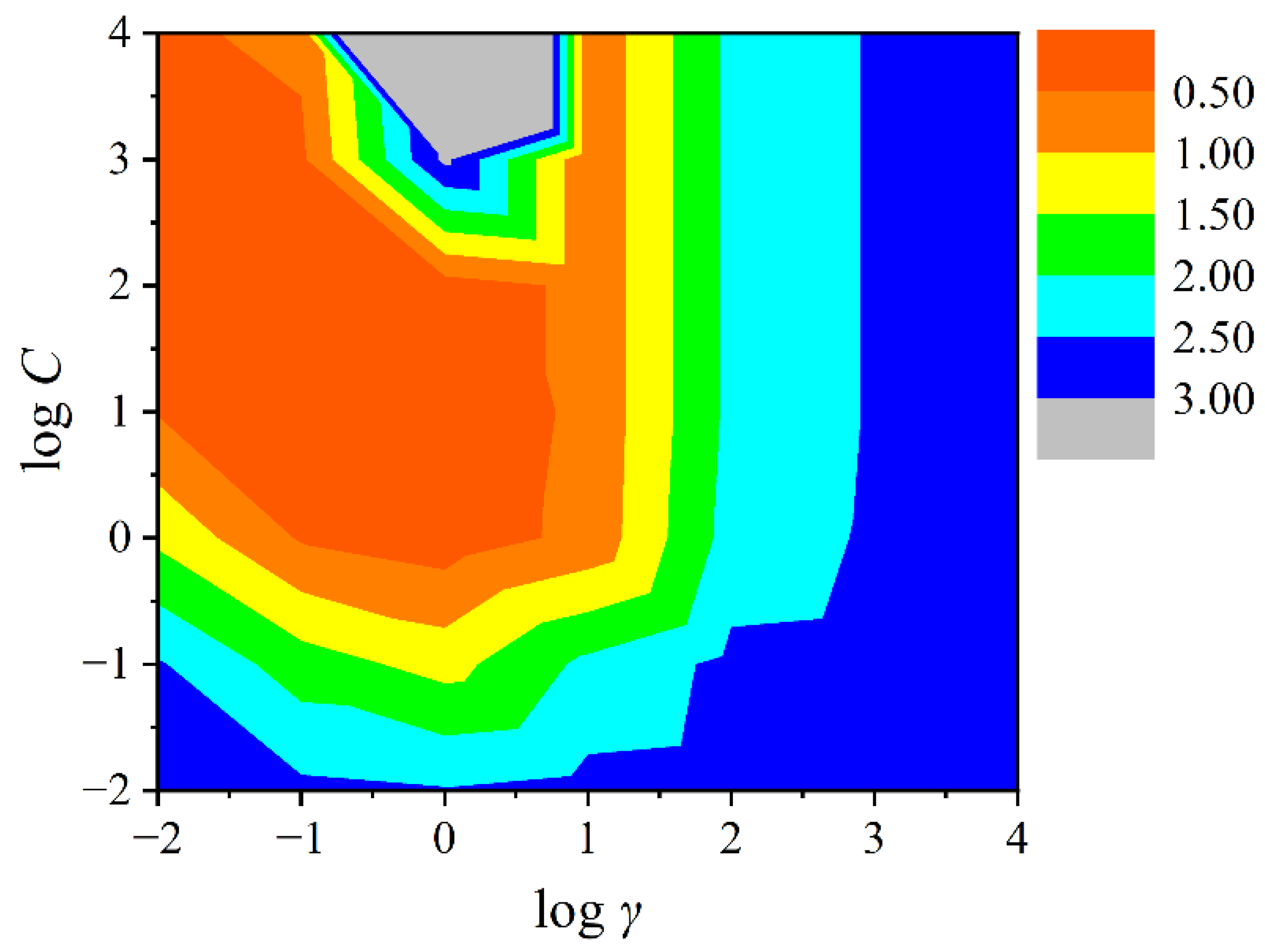
In order to further improve the model’s performance, an SVM model was constructed using R language by the descriptors employed in the MLR model. The kernel function of the SVM method is radial basis function. The complexity and prediction error of the model were determined by searching for the optimal combination of hyperparameters (γ and C), and the optimal model is obtained based on it. In this process, the range of the combination of γ and C was set as 10−2~104, and the grid search method was used to find the optimal combination. The ten-fold cross validation method was used to evaluate the performance of the SVM model. At the same time, the counter map of log γ and log C was drawn to visualize the combination of the hyperparameters.

2.4. Define the Application Domain

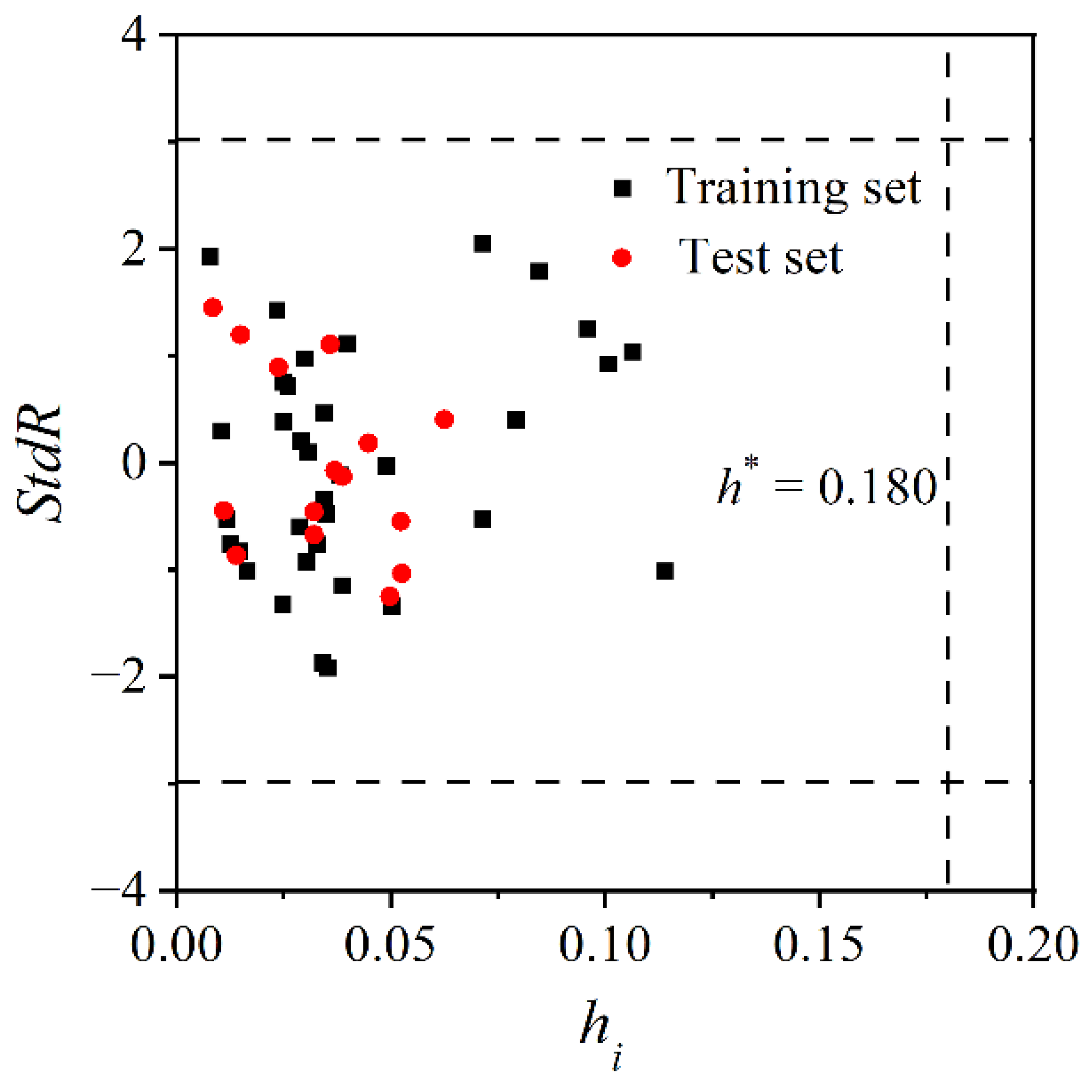
The model application domain was defined using a Williams diagram [33]. If the absolute value of the standardized residual (StdR) of a compound is smaller than 3, it is considered to be well predicted. If the leverage value hi of a compound is larger than the threshold h* (h* = 3 × p/n, p represents the number of molecular structure descriptors, n represents the number of modeling data), this compound may have extreme descriptors that can influence the model construction, so it is identified as a high-influence compound. It should be noted that if the absolute values of StdR of the high-influence compounds are less than 3, this indicates the model has great generalization capability.

3. Results and Discussion

3.1. Model Establishment and Verification

(1)
log KOA model
The linear correlation between log KP and log KOA was obtained:
log KP = (0.643 ± 0.046) × log KOA + (−8.287 ± 0.410)
As shown in Figure 1, log KP positively correlates with log KOA (p < 0.05). This indicates log KOA can be used to roughly predict log KP values. The predictive values are listed in Table 1 and the 95% confidence intervals are provided in Supplementary Materials, Table S1. However, the moderate correlation coefficient (R2 = 0.801) may lead to inaccurate predictive results. QSPR models are further developed.
(2)
MLR model
The QSPR model was established by stepwise MLR method based on quantum chemical descriptors:
log KP = (0.031 ± 0.002) × α + (−24.453 ± 3.684) × Vs.min + (−9.358 ± 0.433)
This model has two molecular descriptors α and Vs.min, both of which have VIF values less than 10 (see Table 2), and there is no multicollinearity in the model (p < 0.05). The predictive log KP values as well as the calculated values of the employed descriptors are shown in Table 1, and the 95% confidence interval of the predictive log KP values can be found in Table S1.
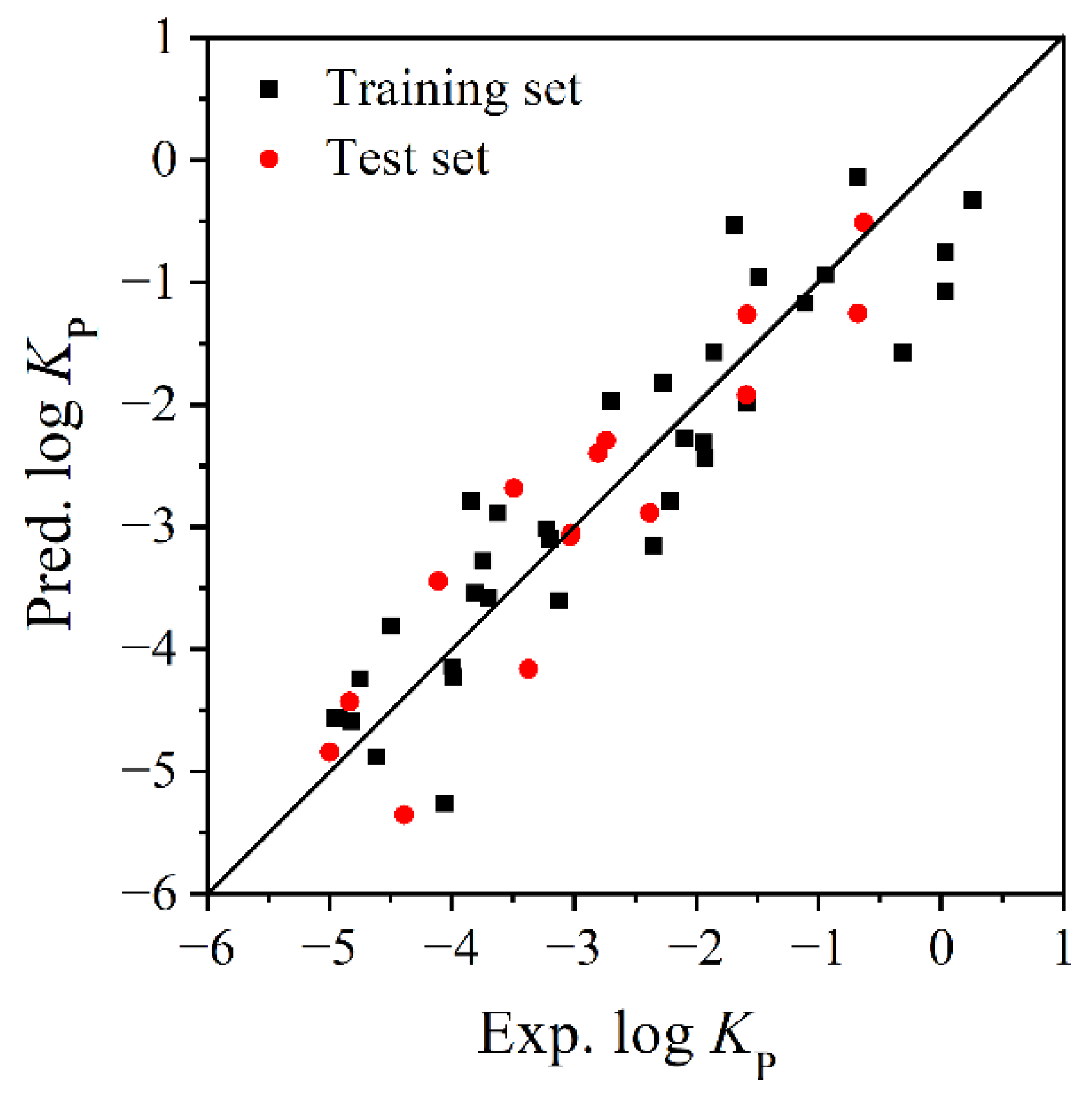
The statistical performance of MLR model based on quantum chemical descriptors has been significantly improved: R2 = 0.847, Q2 = 0.847, and RMSE = 0.584 (Table 3), indicating the model has a good fitting performance. It can be seen from Table 3 that the training set (70%) and validation set (30%) of simulated external validation have similar statistical parameters with the MLR model: R2 = 0.842, Q2 = 0.842, and RMSE = 0.618 (training set); R2 = 0.854, Q2 = 0.847, and RMSE = 0.535 (validation set); R2 = 0.847, Q2 = 0.847, RMSE = 0.584 (MLR model based on whole dataset). The regression coefficients of the descriptors in the model established by the training set are also close to those of the MLR model, 0.031 for α in both models based on training set and the whole dataset; −27.835 and −24.453 for Vs.min for training set and the whole dataset, respectively. Moreover, Roy et al. [44,45] have pointed out a serial criterion to detect the existence of systematic error and to judge the predictive ability. We also applied this criterion to our validation set, and the calculation results were: (1) the ratio of number of positive and negative errors NPE/NNE = 1.143, no larger than 5; the absolute value of mean positive error / mean negative error ABS (MPE/MNE) = 0.903, smaller than 2; the difference between the average absolute error (MAE = 0.438) and absolute of average value (ABS (BIAS) = 0.002) is 0.436, larger than 0.5 × MAE; R2 (ith vs (i − 1)th residuals) = 0.099, smaller than 0.5; R2 (log KP vs. residuals) = 0.029, smaller than 0.5; (2) after removing the two highest residual values (5%), the MAE (0.370) is smaller than 0.1 × log KP range of training set (5.21) and MAE + 3σ (standard deviation of the absolute error, 0.234) is very close to 0.2 × log KP range of training set. These results show that the developed MLR model has no systematic error and good predictive ability. In the leave-one-out cross-validation, the average Q2CV and RMSECV is 0.906 and 0.625, respectively, which further proves the robustness of the developed MLR model [46].
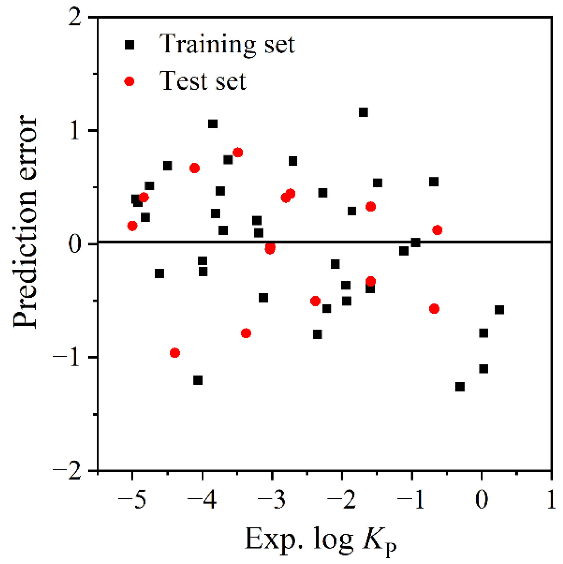
The fitting plot of the experimental log KP values and the predicted log KP values by the MLR model (Figure 2) shows they have great agreement. Figure 3 shows that the predictive errors of log KP are randomly distributed, and they have no dependence on the experimental value. This conclusion can also be verified by the BIAS = 0.000 of the MLR model (Table 3).
(3)
SVM model
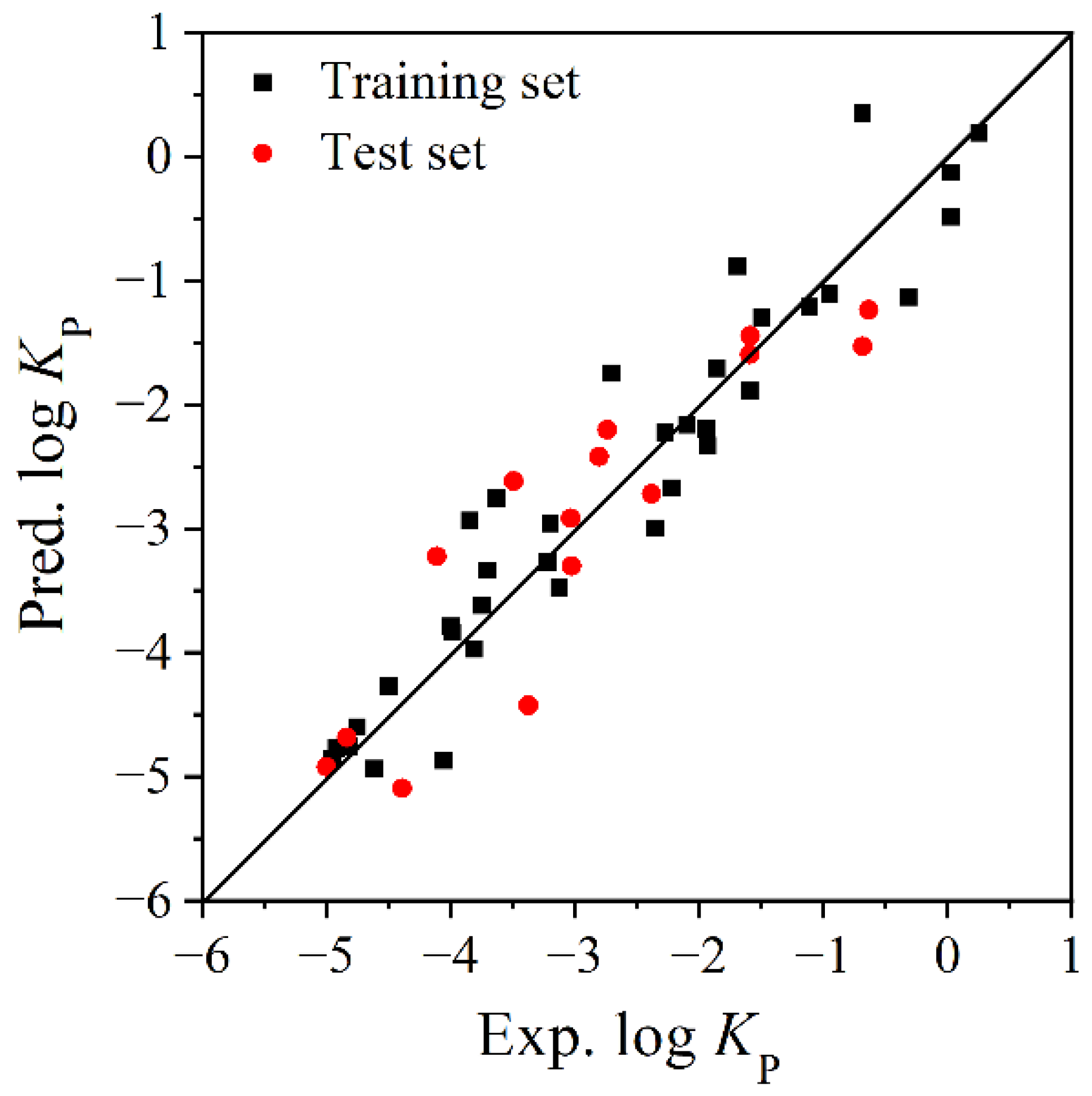
In order to check whether the machine learning method could improve the statistical performance of the model, SVM model is further established basing on the descriptors (α and Vs.min) that are screened by MLR. The contour map of the combination of hyperparameter γ and penalty factors C is shown in Figure 4. It shows that the smallest predictive errors of the model (<0.50) exist in the brown area, and the largest predictive errors appear in the gray area. The optimal combination is γ = 0.1, C = 10, which yields the following evaluation parameters (N represents the number of data points in the data set):
N = 35, R2 = 0.908, RMSE = 0.465, Q2 = 0.853 (training set)
N = 15, R2 = 0.813, RMSE = 0.572, Q2 = 0.818 (validation set)
The model also has good fitting ability and robustness, as shown by the high R2 (0.908) and Q2 (0.853) values. In external validation, both R2 (0.813) and Q2 (0.818) values are greater than 0.8, further indicating a good predictive ability. Figure 5 also shows a good agreement between the experimental log KP values and the predictive values calculated by the SVM model.
(4)
Comparison of the different models
The R2 values of the log KOA model, the MLR model and the SVM model are all greater than 0.8, indicating every model has good fitting ability. In comparison, the MLR model has better performance than the log KOA model. The training set of SVM model obtains the highest R2 value among the three models; however, the R2 of its validation set is relatively lower than that of MLR model. As a black-box model, the prediction of the SVM model is an opaque process which cannot provide more information, such as the relationship between the molecular descriptors and the target endpoint under study, thus limiting its application. Furthermore, the MLR model based on molecular structure descriptors avoids the difficulties of experimental measurement, and is a visual model, making it simpler and more convenient for practical application. According to the comprehensive comparison, the MLR model is considered as the optimal predictive log KP model for the following analysis.

3.2. Characterization of the Model Application Domain

Figure 6 shows the Williams diagram of the MLR model with threshold h* = 0.180. All data points locate at the left of h*, and the absolute values of StdR for all compounds are less than 3, indicating the accurate predictive of this model. Therefore, the MLR model has good applicability and can be used to predict the log KP values of compounds in the descriptor domain (α: 99.753~280.623; Vs.min: −9.535 × 10⁻²~−2.498 × 10⁻²).

3.3. Mechanism Analysis

The MLR model contains two descriptors, the average molecular polarization α and the most negative electrostatic potential on the molecular surface Vs.min. α has the highest correlation with log KP with the correlation coefficient R of 0.839, indicating the great importance of average molecular polarizability in affecting the distribution of PAHs and oxygen/nitrogen derivatives between gas phase and atmospheric particle phase. α characterizes the dispersive interaction between the molecules, and a larger α corresponds to a stronger intermolecular dispersive effect [47,48]. Because of the great distance between molecules in the air, the dispersion interaction mainly occurs between atmospheric particles and chemical molecules. Therefore, a larger α leads to stronger dispersion interactions between chemical molecules and particles, and further results in a larger log KP. Thus, α yields a positive coefficient (0.031) in the model. The second descriptor, Vs.min, shows negative correlation with log KP (the coefficient of −24.453). Vs.min reflects the contribution of molecular electrostatic hydrogen bonds; that is, it reflects the ability of molecules to accept protons to form hydrogen bonds. The smaller Vs.min value indicates a higher electron density and a stronger ability to accept protons to form hydrogen bonds [49,50]. Therefore, PAHs and oxygen/nitrogen derivatives with smaller Vs.min values are more likely to combine with atmospheric particulates which have complex compositions.

3.4. Discussion

Yuan et al. [51] constructed a temperature-dependent QSPR model for predicting the log KP values of 10 PAHs compounds based on molecular structure descriptors and ambient temperature (T). The model included also the descriptor α as well as variable T; however, its statistical performance is not satisfactory: R2 = 0.624, Q2 = 0.624, and RMSE = 0.395. Sun et al. [52] established a Theoretical Linear Solution Energy Relationship (TLSER) model for some organic compounds, including alkanes, alkalic acids, PAHs, O-PAHs and N-PAHs (Table 4), in which KP1 and KP2 represent KP values measured by 190 m3 and 25 m3 smoke chambers, respectively. These models show that dispersion and hydrogen bonding are important factors affecting KP values, which is consistent with the results of this study. However, the TLSER models contain fewer PAH, O-PAH and N-PAH data. Furthermore, the number of descriptors used in this study is less, which makes it easier to apply.

4. Conclusions

In this study, the correlation between the log KP and log KOA of PAHs and their oxygen/nitrogen derivatives is first analyzed, and then QSPR models for log KP prediction are constructed based on quantum chemical descriptors by MLR and SVM algorithms. The QSPR models have better fitting performance, predictive ability and robustness. The mechanism analysis shows that the major factors affecting the distribution of PAHs, O-PAHs, N-PAHs and AZA in the gas and particle phases are intermolecular dispersion and hydrogen bonding. Although the SVM model is slightly superior to the MLR model, it is a black-box model with poor transparency and is dependent on the descriptor screening of MLR process, limiting its further application. In contrast, the MLR model has simple and visualized mathematical expression, bringing convenience to the analysis of the important factors that affect the partitioning of these chemicals between gas and atmospheric particulate phases according to the chemical information carried by the quantum chemical descriptors. Thus, the MLR model can be used to predict the log KP values of other PAHs and oxygen/nitrogen derivatives, with the average molecular polarization within 280.623 and 99.753 and the most negative electrostatic potential on the molecular surface Vs.min within −2.498 and −9.535. The log KP values can provide basic data for their environmental fate and ecological risk assessment.

Supplementary Materials

The following supporting information can be downloaded at: https://www.mdpi.com/article/10.3390/molecules27217608/s1, Table S1: The lower and upper limit of 95% confidence interval of log KOA model, MLR model and SVM model.

Author Contributions

Conceptualization, H.Y. and S.C.; methodology, S.C.; software, Q.W.; validation, Q.W., Z.C. and X.W.; formal analysis, S.C.; investigation, S.C. and Q.W.; resources, H.Y.; data curation, S.C.; writing—original draft preparation, Q.W. and S.C.; writing—review and editing, Q.W. and G.M.; visualization, Q.W.; supervision, H.Y.; project administration, H.Y.; funding acquisition, H.Y. All authors have read and agreed to the published version of the manuscript.

Funding

This research was funded by National Natural Science Foundation of China (21677133, 2217617) and Natural Science Foundation of Zhejiang Province (LY22B070002). The APC was funded by H.Y.

Conflicts of Interest

The authors declare no competing interests.

References

  1. Kim, K.H.; Jahan, S.A.; Kabir, E.; Brown, R.J.C. A review of airborne polycyclic aromatic hydrocarbons (PAHs) and their human health effects. Environ. Int. 2013, 60, 71–80. [Google Scholar] [CrossRef] [PubMed]
  2. Yu, H. Environment carcinogenic polycyclic aromatic hydrocabons: Photochemistry and phototoxicity. J. Environ. Health Sci. Eng. Part. C 2002, 20, 149–183. [Google Scholar] [CrossRef] [PubMed]
  3. Rajpara, R.K.; Dudhagara, D.R.; Bhatt, J.K.; Gosai, H.B.; Dave, B.P.J.M.P.B. Polycyclic aromatic hydrocarbons (PAHs) at the Gulf of Kutch, Gujarat, India: Occurrence, source apportionment, and toxicity of PAHs as an emerging issue. Mar. Pollut. Bull. 2017, 119, 231–238. [Google Scholar] [CrossRef] [PubMed]
  4. Holme, J.A.; Brinchmann, B.C.; Refsnes, M.; Lg, M.; Øvrevik, J. Potential role of polycyclic aromatic hydrocarbons as mediators of cardiovascular effects from combustion particles. Environ. Health 2019, 18, 74. [Google Scholar] [CrossRef] [Green Version]
  5. Mallah, M.A.; Changxing, L.; Mallah, M.A.; Noreen, S.; Liu, Y.; Saeed, M.; Xi, H.; Ahmed, B.; Feng, F.; Mirjat, A.A.; et al. Polycyclic aromatic hydrocarbon and its effects on human health: An overeview. Chemosphere 2022, 296, 133948. [Google Scholar] [CrossRef]
  6. Han, F.; Guo, H.; Hu, J.; Zhang, J.; Ying, Q.; Zhang, H. Sources and health risks of ambient polycyclic aromatic hydrocarbons in China. Sci. Total Environ. 2020, 698, 134229. [Google Scholar] [CrossRef]
  7. Albinet, A.; Leoz-Garziandia, E.; Budzinski, H.; ViIlenave, E. Polycyclic aromatic hydrocarbons (PAHs), nitrated PAHs and oxygenated PAHs in ambient air of the Marseilles area (South of France): Concentrations and sources. Sci. Total Environ. 2007, 384, 280–292. [Google Scholar] [CrossRef] [Green Version]
  8. Bleeker, E.A.J.; Van Der Geest, H.G.; Klamer, H.J.C.; De Voogt, P.; Wind, E.; Kraak, M.H.S. Toxic and genotoxic effects of azaarenes: Isomers and metabolites. Polycycl. Aromat. Compd. 1999, 13, 191–203. [Google Scholar] [CrossRef]
  9. Ma, Y.; Cheng, Y.; Qiu, X.; Lin, Y.; Cao, J.; Hu, D.J.E.P. A quantitative assessment of source contributions to fine particulate matter (PM2.5)-bound polycyclic aromatic hydrocarbons (PAHs) and their nitrated and hydroxylated derivatives in Hong Kong. Environ. Pollut. 2016, 219, 742–749. [Google Scholar] [CrossRef]
  10. Lima, A.L.C.; Farrington, J.W.; Reddy, C.M. Combustion-Derived polycyclic aromatic hydrocarbons in the environment—A review. Environ. Forensics 2005, 6, 109–131. [Google Scholar] [CrossRef]
  11. Huang, R.J.; Zhang, Y.; Bozzetti, C.; Ho, K.F.; Cao, J.J.; Han, Y.; Daellenbach, K.R.; Slowik, J.G.; Platt, S.M.; Canonaco, F.; et al. High secondary aerosol contribution to particulate pollution during haze events in China. Nature 2014, 514, 218–222. [Google Scholar] [CrossRef] [PubMed] [Green Version]
  12. Keyte, I.J.; Albinet, A.; Harrison, R.M. On-road traffic emissions of polycyclic aromatic hydrocarbons and their oxy- and nitro- derivative compounds measured in road tunnel environments. Sci. Total Environ. 2016, 566–567, 1131–1142. [Google Scholar] [CrossRef] [PubMed] [Green Version]
  13. Huang, L.; Chernyak, S.M.; Batterman, S.A. PAHs, nitro-PAHs, hopanes, and steranes in lake trout from Lake Michigan. Environ. Toxicol. Chem. 2014, 33, 1792–1801. [Google Scholar] [CrossRef] [PubMed] [Green Version]
  14. Krzyszczak, A.; Czech, B. Occurrence and toxicity of polycyclic aromatic hydrocarbons derivatives in environmental matrices. Sci. Total Environ. 2021, 788, 147738. [Google Scholar] [CrossRef]
  15. Sun, C.; Qu, L.; Wu, L.; Wu, X.; Sun, R.; Li, Y. Advances in analysis of nitrated polycyclic aromatic hydrocarbons in various matrices. TrAC Trends Anal. Chem. 2020, 127, 115878. [Google Scholar] [CrossRef]
  16. Li, W.; Wang, C.; Shen, H.; Su, S.; Shen, G.; Huang, Y.; Zhang, Y.; Chen, Y.; Chen, H.; Lin, N.; et al. Concentrations and origins of nitro-polycyclic aromatic hydrocarbons and oxy-polycyclic aromatic hydrocarbons in ambient air in urban and rural areas in northern China. Environ. Pollut. 2015, 197, 156–164. [Google Scholar] [CrossRef]
  17. Cai, C.; Li, J.; Wu, D.; Wang, X.; Tsang, D.C.W.; Li, X.; Sun, J.; Zhu, L.; Shen, H.; Tao, S.; et al. Spatial distribution, emission source and health risk of parent PAHs and derivatives in surface soils from the Yangtze River Delta, eastern China. Chemosphere 2017, 178, 301–308. [Google Scholar] [CrossRef]
  18. Qiao, M.; Qi, W.; Liu, H.; Qu, J. Oxygenated, nitrated, methyl and parent polycyclic aromatic hydrocarbons in rivers of Haihe River System, China: Occurrence, possible formation, and source and fate in a water-shortage area. Sci. Total Environ. 2014, 481, 178–185. [Google Scholar] [CrossRef]
  19. Minero, C.; Maurino, V.; Borghesi, D.; Pelizzetti, E.; Vione, D. An overview of possible processes able to account for the occurrence of nitro-PAHs in Antarctic particulate matter. Microchem. J. 2010, 96, 213–217. [Google Scholar] [CrossRef] [Green Version]
  20. Ma, T.; Kong, J.J.; Han, M.S. Review on the pollution status and toxicity effects of nitrated polycyclic aromatic hydrocarbons in the environment. Environ. Chem. 2020, 39, 2430–2440. [Google Scholar]
  21. Zhang, Y.J.; Yun, Y. Oxygenated polycyclic aromatic hydrocarbons in the environment:A review. Environ. Chem. 2021, 40, 150–163. [Google Scholar]
  22. Xu, X.B. Nitro polycyclic aromatic hydrocarbonsRecently discovered direct mutagens and potential carcinogens in the environment. Environ. Chem. 1984, 3, 1–16. [Google Scholar]
  23. Durant, J.L.; Busby, W.F.; Lafleur, A.L.; Penman, B.W.; Crespi, C.L. Human cell mutagenicity of oxygenated, nitrated and unsubstituted polycyclic aromatic hydrocarbons associated with urban aerosols. Mutat. Res. Genet. Toxicol. 1996, 371, 123–157. [Google Scholar] [CrossRef]
  24. Zhang, Q.; Gao, R.; Xu, F.; Zhou, Q.; Wang, W. Role of water molecule in the gas-phase formation process of nitrated polycyclic aromatic hydrocarbons in the atmosphere: A computational study. Environ. Sci. Technol. 2014, 48, 5051–5057. [Google Scholar] [CrossRef] [PubMed]
  25. Idowu, O.; Semple, K.T.; Ramadass, K.; O’Connor, W.; Hansbro, P.; Thavamani, P. Beyond the obvious: Environmental health implications of polar polycyclic aromatic hydrocarbons. Environ. Int. 2019, 123, 543–557. [Google Scholar] [CrossRef]
  26. Yaffe, D.; Cohen, Y.; Arey, J.; Grosovsky, A.J. Multimedia analysis of PAHs and Nitro-PAH daughter products in the Los Angeles basin. Risk Anal. 2008, 72, 1567–1572. [Google Scholar] [CrossRef]
  27. Wang, P.; Wang, S.L.; Fan, C.Q. Atmospheric distribution of particulate- and gas-phase phthalic esters (PAEs) in a Metropolitan City, Nanjing, East China. Chemosphere 1987, 21, 2275–2283. [Google Scholar] [CrossRef]
  28. Harner, T.; Bidleman, T.F. Octanol-air partition coefficient for describing particle/gas partitioning of aromatic compounds in urban air. Environ. Sci. Technol. 1998, 32, 1494–1502. [Google Scholar] [CrossRef]
  29. Finizio, A.; Mackay, D.; Bidleman, T.; Harner, T.J.A.E. Octanol-air partition coefficient as a predictor of partitioning of semi-volatile organic chemicals to aerosols. Atmos. Environ. 1997, 31, 2289–2296. [Google Scholar] [CrossRef]
  30. Cao, S.; Hu, J.; Wu, Q.; Wei, X.; Ma, G.; Yu, H. Prediction study on the distribution of polycyclic aromatic hydrocarbons and their halogenated derivatives in the atmospheric particulate phase. Ecotox. Environ. Safe 2022, 245, 114111. [Google Scholar] [CrossRef]
  31. Hong, H.; Lu, Y.; Zhu, X.; Wu, Q.; Jin, L.; Jin, Z.; Wei, X.; Ma, G.; Yu, H. Cytotoxicity of nitrogenous disinfection byproducts: A combined experimental and computational study. Sci. Total Environ. 2023, 856, 159273. [Google Scholar] [CrossRef] [PubMed]
  32. Wei, X.; Li, M.; Wang, Y.; Jin, L.; Ma, G.; Yu, H. Developing predictive models for carrying ability of micro-plastics towards organic pollutants. Molecules 2019, 24, 1784. [Google Scholar] [CrossRef] [PubMed] [Green Version]
  33. Liu, S.; Jin, L.; Yu, H.; Lv, L.; Chen, C.-E.; Ying, G.-G. Understanding and predicting the diffusivity of organic chemicals for diffusive gradients in thin-films using a QSPR model. Sci. Total Environ. 2020, 706, 135691. [Google Scholar] [CrossRef] [PubMed]
  34. Li, M.; Yu, H.; Wang, Y.; Li, J.; Ma, G.; Wei, X. QSPR models for predicting the adsorption capacity for microplastics of polyethylene, polypropylene and polystyrene. Sci. Rep. 2020, 10, 14597. [Google Scholar] [CrossRef]
  35. Wei, C.; Han, Y.; Bandowe, B.A.M.; Cao, J.; Huang, R.J.; Ni, H.; Tian, J. Occurrence, gas/particle partitioning and carcinogenic risk of polycyclic aromatic hydrocarbons and their oxygen and nitrogen containing derivatives in Xi’an, central China. Sci. Total Environ. 2015, 505, 814–822. [Google Scholar] [CrossRef]
  36. Goss, K.U.; Schwarzenbach, R.P. Linear free energy relationships used to evaluate Equilibrium partitioning of organic compounds. Environ. Sci. Technol. 2001, 35, 1–9. [Google Scholar] [CrossRef]
  37. Nguyen, T.H.; Goss, K.U.; Ball, W.P. Polyparameter linear free energy relationships for estimating the equilibrium partition of organic compounds between water and the natural organic matter in soils and sediments. Environ. Sci. Technol. 2005, 39, 913–924. [Google Scholar] [CrossRef]
  38. Frisch, M.J.; Trucks, G.W.; Schlegel, H.B.; Scuseria, G.E.; Robb, M.A.; Cheeseman, J.R.; Scalmani, G.; Barone, V.; Mennucci, B.; Petersson, G.A.; et al. Gaussian 16, Revision, D.01; Gaussian, Inc.: Wallingford, CT, USA, 2016. [Google Scholar]
  39. Tian, L. GsGrid: Extracting Data from Gaussian Grid File and Grid File Calculation, Version 1.7. Available online: http://gsgrid.codeplex.com (accessed on 31 October 2022).
  40. Zang, Q.D.; Mansouri, K.; Williams, A.J. In silico prediction of physicochemical properties of environmental chemicals using molecular fingerprints and machine learning. J. Chem. Inf. Model 2016, 57, 36–49. [Google Scholar] [CrossRef]
  41. Pallant, J. SPSS Survival Manual: A step by step guide to data analysis using IBM SPSS. Aust. N. Z. J. Public Health 2013, 37, 597–598. [Google Scholar]
  42. Guidance Document on the Validation of (Quantitative) Structure-Activity Relationship [(Q)SAR] Models; OECD Environment Health and Safety Publications Series on Testing and Assessment, No. 69; OECD: Paris, France, 2007.
  43. Hall, M.; Frank, E.; Holmes, G.; Pfahringer, B.; Reutemann, P.; Witten, I.H. The WEKA data mining software: An update. ACM SIGKDD Explor. Newsl. 2009, 11, 10–18. [Google Scholar] [CrossRef]
  44. Roy, K.; Ambure, P.; Aher, R.B. How important is to detect systematic error in predictions and understand statistical applicability domain of QSAR models? Chemometr. Intell. Lab. 2017, 162, 44–54. [Google Scholar] [CrossRef]
  45. Roy, K.; Das, R.N.; Ambure, P.; Aher, R.B. Be aware of error measures. Further studies on validation of predictive QSAR models. Chemometr. Intell. Lab. Syst. 2016, 152, 18–33. [Google Scholar]
  46. Tropsha, A.; Gramatica, P.; Gombar, V.K. The importance of being earnest: Validation is the absolute essential for successful application and interpretation of QSPR models. QSAR Comb. Sci. 2003, 22, 69–77. [Google Scholar] [CrossRef]
  47. Huang, X.X.; Yang, H.W. Study on the relationship between octanol-air partition coefficient and molecular structure of PCBs. J. Beijing Union Univ. 2014, 28, 34–39. [Google Scholar]
  48. Yu, H.Y.; Chen, W.; Liang, C.C. Predicting the n-octanol/air partitioning coefficients of selected polybrominated diphenyl ethers and their metabolites. J. Zhejiang Norm. Univ. 2015, 38, 266–272. [Google Scholar]
  49. Zou, J.W.; Zhang, B.; Hu, G.X. QSPR studies on the physicochemical properties of polycyclic aromatic hydrocarbons—The application of theoretical descriptors derived from electrostatic potentials on molecular surface. Acta Chem. 2004, 62, 241–246. [Google Scholar]
  50. Zou, J.W.; Jiang, Y.J.; Hu, G.X. QSPR (activity) relationship of polychlorinated biphenyls. Acta Phys. Chem. 2005, 21, 267–272. [Google Scholar]
  51. Yuan, Q.; Ma, G.C.; Xu, T.; Serge, B.; Yu, H.Y.; Chen, J.R.; Lin, H.J. Developing QSPR model of gas/particle partition coefficients of neutral poly-/perfluoroalkyl substances. Atmos. Environ. 2016, 143, 270–277. [Google Scholar] [CrossRef]
  52. Sun, C.; Feng, L. A method for estimating the air/particulate matter partition coefficient of organic matter. Sci. Bull. 2005, 50, 961–963. [Google Scholar]
Figure 1. The fitting plot between experimental log KP values and log KOA values.
Molecules 27 07608 g001
Figure 2. Fitting plot of experimental and predictive log KP values by MLR model.
Molecules 27 07608 g002
Figure 3. The distribution of predictive log KP errors by MLR model.
Molecules 27 07608 g003
Figure 4. Contour map of the combination of hyperparameter (γ) and penalty factor (C) in the SVM model.
Molecules 27 07608 g004
Figure 5. Fitting plot of experimental and predictive log KP values by SVM model.
Molecules 27 07608 g005
Figure 6. Williams diagram of MLR model.
Molecules 27 07608 g006
Table 1. Experimental and predicted log KP values, log KOA values, and molecular structure descriptors employed in the QSAR model for 50 PAHs and their oxygen/nitrogen derivatives a.
CompoundAbbreviationslog KPlog KOAαVS.min (×10−2)
Exp.Pred.
(log KOA)
Pred.
(MLR Model)
Pred.
(SVM Model)
1,2,3,4-TetrahydronaphthaleneTH-NAPH−4.060−5.231 −5.184−4.8674.75108.571−3.397
NaphthaleneNAPH b−4.392−5.038 −5.239−5.0935.05112.345−2.698
2-Methylnaphthalene2-MNAPH b−5.001−4.729 −4.738−4.9205.53126.847−2.924
1-Methylnaphthalene1-MNAPH−4.617−4.716 −4.789−4.9325.55125.047−2.944
BiphenylBIPH−4.955−4.484 −4.469−4.8515.91137.036−2.739
1,3-Dimethylnaphthalene1,3DMNAPH b−4.837−4.407 −4.330−4.6806.03139.231−3.030
AcenaphthyleneACEY−4.921−4.253 −4.476−4.7666.27134.493−3.034
AcenaphtheneACEN−4.821−4.401 −4.511−4.7506.04132.491−3.141
FluoreneFLUO−4.756−4.047 −4.163−4.5996.59145.606−2.912
PhenanthrenePHE−4.500−3.642 −3.724−4.2687.22162.006−2.643
AnthraceneANT−3.811−3.725 −3.459−3.9677.09170.616−2.639
2-Methylphenanthrene2-MPHE−3.747−3.461 −3.205−3.6147.50177.433−2.820
3,6-Dimethylphenanthrene3,6-DMPHE−3.847−3.120 −2.728−2.9308.03191.260−3.031
FluorantheneFLUA−3.223−2.754 −2.946−3.2668.60186.008−2.796
PyrenePYR b−3.027−3.017 −2.950−3.3008.19187.779−2.555
ReteneRET−2.703−2.689 −1.919−1.7438.70217.138−3.080
Benzo[a]anthraceneBaA b−1.592−2.451 −1.828−1.5939.07223.989−2.590
Benzo[e]pyreneBeP−0.316−0.984 −1.513−1.13011.35234.532−2.550
Benzo[a]pyreneBaP0.028−1.300 −1.016−0.48210.86250.507−2.568
Indeno [1,2,3-cd]pyreneIcdP0.255−0.856 −0.2840.19211.55272.695−2.774
Dibenzo[a,h]anthraceneDahA−0.687−0.708 −0.0940.35211.78280.623−2.553
Benzo[g,h,i]peryleneBghiP0.028−0.888 −0.702−0.12711.50261.269−2.498
1-Indanone1-IND−3.998−4.542 −4.235−3.7845.8299.753−8.388
1,4-Naphthoquinone1,4-NQ−3.990−2.625 −4.261−3.8348.80113.590−6.535
1-Naphthaldehyde1-NALD b−4.111−3.680 −3.506−3.2247.16127.809−7.844
2-Biphenylcarboxaldehyde2-BPCA b−3.491−3.236 −2.760−2.6157.85149.944−8.101
9-Fluorenone9-FLU−3.630−3.050 −2.959−2.7488.14148.889−7.418
1,2-Acenaphthenequinone1,2-ACEQ−3.196−2.625 −3.180−2.9538.80138.303−7.854
9,10-Anthraquinone9,10-AQ b−2.382−2.233 −2.902−2.7189.41159.881−6.271
1,8-Naphtalic anhydride1,8-NA b−3.033−3.243 −3.140−2.9127.84141.118−7.659
4H-Cyclopenta[d,e,f]phenanthrenone4-CPHE b−2.739−2.110 −2.345−2.2019.60170.679−7.191
2-Meth-9,10-anthraquinone2-MAQ−1.944−1.383 −2.362−2.19410.73175.048−6.566
Benzo[a]florenoneBAFLU b−1.590−1.660 −1.322−1.44210.30203.092−7.291
7H-Benzo[d,e]anthracene-7-oneBdeAQ b−0.682−1.608 −1.328−1.52710.38199.470−7.715
Benzo[a]anthracene-7,12-dioneBaAQ−1.112−0.373 −1.231−1.21112.30214.077−6.284
5,12-Naphthacenequinone5,12-NQ−0.949−0.296 −1.006−1.10512.42219.462−6.523
6H-Benzo[c,d]pyren-6-oneBcdPQ b−0.635−0.701 −0.592−1.23111.79222.901−7.780
1-Nitronaphthalene1-NNAP−3.703−3.571 −3.635−3.3337.33129.792−7.060
2-Nitrobiphenyl2-NBP−2.352−3.301 −3.184−2.9937.75151.356−6.187
5-Nitroacenaphthene5-NACE−2.219−3.017 −2.867−2.6718.19151.022−7.526
2-Nitrofluorene2-NFLU−1.932−3.178 −2.501−2.3297.94167.360−6.969
9-Nitrophenanthrene9-NPHE−2.098−2.342 −2.324−2.1589.24177.214−6.454
9-Nitroanthracene9-NANT−1.858−1.943 −1.660−1.7039.86190.063−7.545
1-Nitropyrene1-NPYR−1.496−1.255 −1.048−1.29510.93211.741−7.317
2,7-Dinitrofluorene2,7-DNFLU−1.595−1.647 −2.037−1.88810.32187.649−6.309
6-Nitrochrysene6-NCHR−1.696−0.933 −0.604−0.87911.43232.917−6.475
QuinolineQUI−3.127−4.298 −3.731−3.4756.20107.069−9.535
Benzo[h]quinolineBhQ b−2.804−2.767 −2.483−2.4178.58156.877−8.358
AcridineACR−2.275−2.522 −1.969−2.2228.96165.008−9.437
CarbazoleCAR b−3.372−2.471 −4.071−4.4239.04145.738−3.265
a α (a.u.) represents the average molecular polarizability; Vs.min (eV) represents the most negative electrostatic potential on the molecular surface; b as the validation set in simulated external validation.
Table 2. The coefficients, t-test (t value), significance level (p value) and variance inflation factor (VIF value) of each descriptor in the MLR model.
ParameterCoefficienttpVIF
α0.03115.839<0.0011.056
Vs.min−24.453−6.638<0.0011.056
Table 3. Statistical parameters of the MLR model and the simulated external validation.
NR2Q2RMSEBIASMAEMPEMNE
MLR model500.8470.8470.5840.0000.4911.119−1.197
Training set350.8420.8420.6180.0000.5091.162−1.259
Validation set150.8540.8470.5350.0020.4380.807−0.961
Table 4. Comparison of literature models.
CompoundModelCharacterization ResultsReferences
PAHslog KP = (0.018 ± 0.003) × α + (−0.080 ± 0.033) × T + (18.245 ± 9.979)N = 28, R2 = 0.624,
Q2 = 0.624, RMSE = 0.395
[45]
Organic chemicalslog (103 KP1) = −17.426 + 0.406 × d + 0.058 × α − 0.580 × EHOMO + 10.236 × qH+N = 15, R2 = 0.971,
Q2 = 0.971, RMSE = 0.185
[46]
log (103 KP2) = −21.307 + 0.162 × d + 0.0424 × α − 1.531 × EHOMO − 0.582 × ELUMON = 17, R2 = 0.839,
Q2 = 0.839, RMSE = 0.634
PAHs,
O-PAHs,
N-PAHs
log KP = (0.031 ± 0.002) × α + (−24.453 ± 3.684) × Vs.min + (−9.358 ± 0.433)N = 50, R2 = 0.847,
Q2 = 0.847, RMSE = 0.584
This research
Publisher’s Note: MDPI stays neutral with regard to jurisdictional claims in published maps and institutional affiliations.