Abstract
The intrinsic dynamic and static nature of noncovalent Br-∗-Br interactions in neutral polybromine clusters is elucidated for Br4–Br12, applying QTAIM dual-functional analysis (QTAIM-DFA). The asterisk (∗) emphasizes the existence of the bond critical point (BCP) on the interaction in question. Data from the fully optimized structures correspond to the static nature of the interactions. The intrinsic dynamic nature originates from those of the perturbed structures generated using the coordinates derived from the compliance constants for the interactions and the fully optimized structures. The noncovalent Br-∗-Br interactions in the L-shaped clusters of the Cs symmetry are predicted to have the typical hydrogen bond nature without covalency, although the first ones in the sequences have the vdW nature. The L-shaped clusters are stabilized by the n(Br)→σ*(Br–Br) interactions. The compliance constants for the corresponding noncovalent interactions are strongly correlated to the E(2) values based on NBO. Indeed, the MO energies seem not to contribute to stabilizing Br4 (C2h) and Br4 (D2d), but the core potentials stabilize them, relative to the case of 2Br2; this is possibly due to the reduced nuclear–electron distances, on average, for the dimers.
1. Introduction
Halogen bonding is of current and continuous interest [1,2]. A lot of information relevant to halogen bonding has been accumulated so far [3]. Halogen bonding has been discussed on the basis of the shorter distances between halogen and other atoms in crystals [4,5,6]. The short halogen contacts are found in two types: symmetric (type I) and bent (type II) geometries. The bonding has also been investigated in the liquid [7,8] and gas [9] phases. The nature of halogen bonding has been discussed based on the theoretical background on the molecular orbital description for the bonding and the σ-hole developed on the halogen atoms, together with the stability of the structural aspects [10]. We also reported the dynamic and static nature of Y–X---π(C6H6) interactions recently [11]. Halogen bonding is applied to a wide variety of fields in chemical and biological sciences, such as crystal engineering, supramolecular soft matters, and nanoparticles. Efforts have been made to unify and categorize the accumulated results and establish the concept of halogen bonding [3,12,13,14,15].
Structures of halogen molecules (X2) have been reported, as determined by X-ray crystallographic analysis for X = Cl, Br, and I [16,17,18]. The behavior of bromine–bromine interactions has been reported for the optimized structures of Br2–Br5 in the neutral and/or charged forms, together with Br1, so far [19,20]. Figure 1 draws the observed structure of Br2, for example. The bromine molecules seem to exist as a zig-zag structure in the infinite chains in crystals. One would find the linear alignment of three Br atoms in an L-shaped dimer ((Br2)2; Br4) and the linear alignment of four Br atoms in a double L-shaped trimer ((Br2)3; Br6) in a planar Br2 layer in addition to Br2 itself. The linear four Br atoms are located in the two L-shaped dimers of Br6, overlapped at the central Br2. While the L-shaped dimers seem to construct the zig-zag type infinite chains, the linear four Br atoms construct linear infinite chains. The attractive np(Br)→σ*(Br–Br) σ(3c–4e) (three center–four electron interaction of the σ-type) and np(Br)→σ*(Br–Br)←np(Br) σ(4c–6e) must play a very important role to stabilize Br4 and Br6, respectively, where np(Br) stands for the p-type nonbonding orbital of Br in the plane, perpendicular to the molecular Br2 axis, and σ*(Br–Br) is the σ*-orbital of Br2. The crystal structures of Cl2 and I2 are very similar to that of Br2.
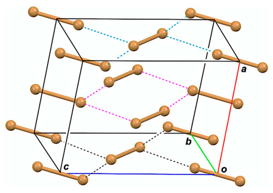
Figure 1.
Structure of Br2, determined by X-ray crystallographic analysis [17].
We have been very interested in the behavior of halogen bonding in polyhalogen clusters, together with the structures. How can the interactions in the polyhalogen clusters be clarified? We propose QTAIM dual-functional analysis (QTAIM-DFA) [21,22,23,24,25] based on the quantum theory of atoms in molecules (QTAIM) approach introduced by Bader [26,27] to classify and characterize the various interactions effectively [28]. In QTAIM-DFA, Hb(rc) are plotted versus Hb(rc) − Vb(rc)/2 (=(ћ2/8m)∇2ρb(rc) (see Equation (SA2) in the supplementary materials), where ρb(rc), Hb(rc), and Vb(rc) stand for the charge densities, total electron energy densities, and potential energy densities, respectively, at bond critical points (BCPs, ∗) on the bond paths (BPs) in this paper [26]. The kinetic energy densities at BCPs will be similarly denoted by Gb(rc) [26]. A chemical bond or an interaction between Br and Br is denoted by Br-∗-Br in this work, where the asterisk emphasizes the existence of a BCP on a BP for Br–Br [26,27]. In our treatment, data from the fully optimized structures are plotted together with those from the perturbed structures around the fully optimized ones. The static nature of the interactions corresponds to the data from the fully optimized structures, which are analyzed using polar coordinate (R, θ) representation [21,22,23,24,25]. On the other hand, the dynamic nature originates based on the data from both the perturbed and fully optimized structures [21,22,23,24,25]. The plot is expressed by (θp, κp), where θp corresponds to the tangent line and κp is the curvature of the plot. θ and θp are measured from the y-axis and the y-direction, respectively. We call (R, θ) and (θp, κp) the QTAIM-DFA parameters [29].
Interactions are classified by the signs of ∇2ρb(rc) and Hb(rc), based on the QTAIM approach. The interactions are called shard shell (SS) interactions when ∇2ρb(rc) < 0 and closed-shell (CS) interactions when ∇2ρb(rc) > 0 [26]. In particular, CS interactions are called pure CS (p-CS) interactions when Hb(rc) > 0 and ∇2ρb(rc) > 0. We call interactions where Hb(rc) < 0 and ∇2ρb(rc) > 0 regular CS (r-CS) interactions, which clearly distinguishes these interactions from the p-CS interactions. The signs of ∇2ρb(rc) can be replaced by those of Hb(rc) − Vb(rc)/2 because (ћ2/8m)∇2ρb(rc) = Hb(rc) − Vb(rc)/2 (see Equation (SA2) in the supporting information). Indeed, Hb(rc) − Vb(rc)/2 = 0 corresponds to the borderline between the classic covalent bonds of SS and the noncovalent interactions of CS, but Hb(rc) = 0 appears to be buried in the noncovalent interactions of CS. As a result, it is difficult to characterize the various CS interactions based on the signs of Hb(rc) − Vb(rc)/2 and/or Hb(rc). In QTAIM-DFA, the signs of the first derivatives of Hb(rc) − Vb(rc)/2 and Hb(rc) (d(Hb(rc) − Vb(rc)/2)/dr and dHb(rc)/dr, respectively, where r is the interaction distance) are used to characterize CS interactions, in addition to those of Hb(rc) − Vb(rc)/2 and Hb(rc), after analysis of the plot. While the former corresponds to (θp, κp), the latter does to (R, θ). The analysis of the plots enables us to characterize the various CS interactions more effectively. Again, the details are explained later.
The perturbed structures necessary for QTAIM-DFA can be generated. Among them, a method employing the coordinates corresponding to the compliance constants Cii for internal vibrations is shown to be highly reliable to generate the perturbed structures [30,31,32,33,34,35,36,37,38,39]. The method, which we proposed recently, is called CIV. The dynamic nature of interactions based on the perturbed structures with CIV is described as the “intrinsic dynamic nature of interactions” since the coordinates are invariant to the choice of coordinate system. Rough criteria that distinguish the interaction in question from others are obtained by applying QTAIM-DFA with CIV to standard interactions. QTAIM-DFA and the criteria are explained in the appendix of the supplementary materials using Schemes SA1–SA3, Figures SA1 and SA2, Table SA1, and Equations (SA1)–(SA7). The basic concept of the QTAIM approach is also explained.
QTAIM-DFA, using the perturbed structures generated with CIV, is well-suited to elucidate the intrinsic dynamic and static nature of halogen–halogen interactions in the polyhalogen clusters. As the first step to clarify the nature of various types of halogen–halogen interactions in the polyhalogen clusters, the nature of each bromine–bromine interaction in the neutral polybromine clusters is elucidated by applying QTAIM-DFA. Various types of structures and interactions are found in the optimized structures of polybromine clusters, other than those observed in the crystals. Here, we present the results of investigations on the polybromine clusters, together with the structural feature, elucidated with QTAIM-DFA and QC calculations.
2. Methodological Details in Calculations
The structures were optimized by employing Gaussian 09 programs [40]. The 6-311+G(3df) basis [41,42,43,44] set was applied to optimize the structures of neutral polybromine clusters, Br2–Br12. The Møller–Plesset second-order energy correlation (MP2) level [45,46,47] was applied for the optimizations. Optimized structures were confirmed by frequency analysis. The results of the frequency analyses were employed to calculate the Cij values and coordinates corresponding to Cii [30,34,35,36]. The ρb(rc), Hb(rc) − Vb(rc)/2 (=(ћ2/8m)∇2ρb(rc)), and Hb(rc) values were calculated using the Gaussian 09 program package [40], with the same method applied to the optimizations. Data were analyzed with the AIM2000 [48,49] and AIMAll [50] programs.
Coordinates corresponding to the compliance constants for an internal coordinate i of the internal vibrations (Ci) were employed to generate the perturbed structures necessary in QTAIM-DFA [21,22,23,24,25]. Equation (1) explains the method to generate the perturbed structures with CIV. An i-th perturbed structure in question (Siw) was generated by the addition of the coordinates (Ci) corresponding to Cii to the standard orientation of a fully optimized structure (So) in the matrix representation. The coefficient giw in Equation (1) controls the difference in structures between Siw and So: giw are determined to satisfy Equation (2) for the interaction in question, where r and ro show the distances in question in the perturbed and fully optimized structures, respectively, with ao of Bohr radius (0.52918 Å) [21,22,23,24,25,30].
Siw = So + giw × Ci
r = ro + wao (w = (0), ±0.05 and ±0.1; ao = 0.52918 Å)
y = co + c1x + c2x2 + c3x3 (Rc2: square of correlation coefficient)
In the QTAIM-DFA treatment, Hb(rc) are plotted versus Hb(rc) − Vb(rc)/2 for the data of five points of w = 0, ±0.05, and ±0.1 in Equation (2). Each plot is analyzed using a regression curve of the cubic function, as shown in Equation (3), where (x, y) = (Hb(rc) − Vb(rc)/2, Hb(rc)) (Rc2 (square of correlation coefficient) > 0.99999 in the norm) [25].
3. Results and Discussion
3.1. Structural Optimizations of Polybromine Clusters, Br6–Br12
Structures of the neutral Br2–Br12 clusters were optimized with MP2/6-311+G(3df). The structural parameters for the optimized structures of minima for Br2–Br6 and Br8–Br12 are collected in Tables S1 and S2, respectively. Some transition states (TSs) for Br4 and Br6 were also calclaterd. The notation of Cs-Lm (m = 1–5) is used for the linear L-shaped clusters of the Cs symmetry, where m stands for the number of noncovalent interactions in Br2m+2 (m = 1–5). Cyclic structures are also optimized, retaining the higher symmetries. The optimized structures are not shown in figures, but they can be found in the molecular graphs with the contour maps of ρ(r) for the linear-type bromine clusters Br4–Br12 (Cs-Lm (m = 1–5)) and for the cyclic bromine clusters Br4–Br12, drawn on the optimized structures with MP2/6-311+G(3df) [51]. The energies for the formation of Br4–Br6 and Br8–Br12 are given in Tables S1 and S2, respectively, from the components (∆E = E(Br2k) − kE(Br2)) on the energy surfaces (∆EES) and those with the collections of zero-point energies (∆EZP). The ∆EZP values were plotted versus ∆EES. The plot is shown in Figure S1, which gives an excellent correlation (y = 0.940x + 0.129; Rc2 (square of correlation coefficient) = 0.9999) [52]. Therefore, the ∆EES values are employed for the discussion.
The behavior of the neutral dibromine clusters (Br4) is discussed first. Three structures were optimized for Br4 as minima with some TSs. The minima are the L-shaped structure of Cs symmetry (Br4 (Cs-L1)) [19], the cyclic structure of C2h symmetry (Br4 (C2h)), and the tetrahedral type of D2d symmetry (Br4 (D2d)). A TS of the Cs symmetry was detected between Br4 (Cs-L1) and Br4 (C2h), and two TSs of the C1 symmetry were between Br4 (C2h) and Br4 (D2d) and between Br4 (D2d) and Br4 (Cs-L1). They are called TS (Cs: Cs, C2h), TS (C1: C2h, D2d), and TS (C1: D2d, Cs), respectively. The three minima will be converted to each other through the three TSs. A TS between Br4 (Cs-L1) and its topological isomer was also detected, which is called TS (C2v: Cs, Cs); however, further effort was not made to search for similar TSs between Br4 (C2h) and its topological isomer and between Br4 (C2d) and its topological isomer.
Figure 2 draws the energy profiles for the optimized structures of minima, Br4 (Cs-L1), Br4 (C2h), and Br4 (D2d), together with the TSs TS (Cs: Cs, C2h), TS (Cs: C2h, D2d), TS (C1: C2d, Cs), and TS (C2v: Cs, Cs). The optimized structures are not shown in the figures, but they can be found in the molecular graphs shown in Figure 2, illustrated on the optimized structures. All BCPs expected are detected clearly, together with RCPs and a CCP [26]. The ΔEES value of −10.7 kJ mol−1 for the formation of Br4 (Cs-L1) seems very close to the border area between the vdW and typical hydrogen bond (t-HB) adducts. The driving force for the formation of Br4 (Cs-L1) must be Br3 σ(3c–4e) of the np(Br)→σ*(Br–Br) type. The interactions in Br4 (C2h) and Br4 (D2d) seem very different from those in Br4 (Cs-L1). The ΔEES values of Br4 (C2h) (−8.0 kJ mol−1) and Br4 (D2d) (−9.1 kJ mol−1) are close to that for Br4 (Cs-L1) (−10.7 kJ mol−1). Moreover, the values for TS (Cs: Cs, C2h) (−7.4 kJ mol−1), TS (C1: C2h, D2d) (−7.6 kJ mol−1), TS (C1: D2d, Cs) (−7.0 kJ mol−1), and TS (C2v: Cs, Cs) (−8.7 kJ mol−1) are not so different from those for the minima.
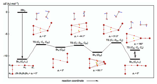
Figure 2.
Energy profile with molecular graphs for the structures of Br4 clusters, optimized with MP2/6-311+G(3df).
In the case of Br6, three structures of the linear Cs symmetry (Br6 (Cs-L2)), the linear C2 symmetry (Br6 (C2)), and the cyclic C3h symmetry (Br6 (C3h-c)) were optimized typically as minima. The linear Br6 clusters of C2h symmetry (Br6 (C2h)) and C2v symmetry (Br6 (C2v)), similar to Br6 (C2), were also optimized, of which the torsional angles, ϕ(1Br2Br5Br6Br) (=ϕ3), were 0° and 180°, respectively. One imaginary frequency was detected for each; therefore, they are assigned to TSs between Br6 (C2) and the topological isomer on the different reaction coordinates. Further effort was not made to search for TSs.
The ΔEES value for Br6 (Cs-L2) was predicted to be −22.6 kJ mol−1. The magnitude is slightly larger than the double value for Br4 (Cs-L1) (∆EES = −10.7 kJ mol−1). Two types of σ (3c–4e) operate to stabilize Br6 (Cs-L2). One, σ(3c–4e), seems similar to that in Br4 (Cs-L1), but the other would be somewhat different. Namely, the second interaction would contribute to ∆EES somewhat more than that of the first one in the formation of Br6 (Cs-L2). On the other hand, the linear interaction in Br6 (C2) can be explained by σ(4c–6e) of the np(Br)→σ*(Br–Br)←np(Br) type. The magnitude of ∆EES of Br6 (C2) seems slightly smaller than that of Br6 (Cs-L2) but is very close to the double value for Br4 (Cs-L1). The magnitude of ∆EES for Br6 (C3h-c) is close to the triple value of Br4 (Cs-L1). One finds triply degenerated σ(3c–4e) interactions in Br6 (C3h-c). The similarity in the interactions for Br4 (Cs-L1), Br6 (C2), and Br6 (C3h-c) will be discussed again later. The magnitudes of ∆EES become proportionally larger to the size of the clusters, as shown in Figures S1 and S2. The ΔEES values are plotted versus k in Br2k (2 ≤ k ≤ 6) for the Cs-Lm type. The results are shown in Figure S2. Contributions from inner σ(3c–4e) (named rin) to ΔEES seem slightly larger than those from σ(3c–4e) in the front end and end positions (named r2 and rω, respectively).
After examination of the optimized structures, the next extension is to clarify the nature of Br-∗-Br interactions by applying QTAIM-DFA. The contour plots are discussed next.
3.2. Molecular Graphs with Contour Plots of Polybromine Clusters
Figure 3 illustrates the molecular graphs with contour maps of ρ(r) for the linear type of Br4 (Cs-L1)–Br12 (Cs-L5), drawn on the structures optimized with MP2/6-311+G(3df). Figure 4 draws the molecular graphs with contour maps of ρ(r) for Br4–Br12, other than those for Br4 (Cs-L1)–Br12 (Cs-L5), calculated with MP2/6-311+G(3df) [53,54] (see also Figure S3). All BCPs expected are detected clearly, together with RCPs and a CCP containing those for noncovalent Br-∗-Br interactions, which are located at the (three-dimensional) saddle points of ρ(r).
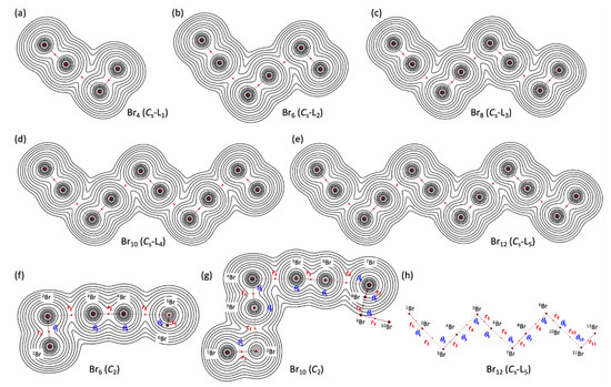
Figure 3.
Molecular graphs with contour plots of ρ(r) for the linear-type bromine clusters of Br4–Br12, calculated with MP2/6-311+G(3df). (a–e) for the linear Cs-Lm type, (f,g) for the C2 type, and (h) for the notations of atoms, bonds, and angles, exemplified by B12 (Cs-L5). BCPs are denoted by red dots, and BPs (bond paths) are by pink lines. Bromine atoms are in reddish-brown.
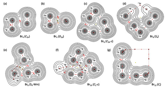
Figure 4.
Molecular graphs with contour plots of ρ(r) for the cyclic bromine clusters of Br4–Br12, (a–g), calculated with MP2/6-311+G(3df). BCPs are denoted by red dots, RCPs (ring-critical points) by yellow dots, CCPs (cage-critical points) by blue dots, and BPs (bond paths) by pink lines. See ref. [55] for (a).
3.3. Survey of the Br-∗-Br Interactions in Polybromine Clusters
As shown in Figure 2, Figure 3 and Figure 4, the BPs in Br4–Br12 seem almost straight. The linearity is confirmed by comparing the lengths of BPs (rBP) with the corresponding straight-line distances (RSL). The rBP and RSL values are collected in Table S3, together with the differences between them, ΔrBP (=rBP − RSL). The magnitudes of ΔrBP are less than 0.01 Å, except for r2 in Br4 (C2v) (ΔrBP = 0.014 Å), r3 in Br8 (S4-Wm) (0.014 Å), and r2 in Br10 (C2-c) (0.012 Å). Consequently, all BPs in Br4–Br12 can be approximated as straight lines.
The ρb(rc), Hb(rc) − Vb(rc)/2 (=(ћ2/8m)∇2ρb(rc)), and Hb(rc) values are calculated for the Br-∗-Br interactions at BCPs in the structures of Br2–Br12, optimized with MP2/6-311+G(3df) [53,54,55]. Table 1 collects the values for the noncovalent Br-∗-Br interactions in Br4–Br12 of the Cs-Lm type. Table 2 summarizes the values for the noncovalent Br-∗-Br interactions in Br4–Br12, other than those of the Cs-Lm type. Hb(rc) are plotted versus Hb(rc) − Vb(rc)/2 for the data shown in Table 1 and Table 2, together with those from the perturbed structures generated with CIV. Figure 5 shows the plots for the noncovalent Br-∗-Br interactions and covalent Br-∗-Br bonds, exemplified by Br10 (Cs-L4).

Table 1.
The ρb(rc), Hb(rc) − Vb(rc)/2 (=(ћ2/8m)∇2ρb(rc)), and Hb(rc) values and QTAIM-DFA parameters for Br-∗-Br at BCPs in Br4 (Cs-L1)–Br12 (Cs-L5), together with Br10 (C2) and Br2, evaluated with MP2/6-311+G(3df) 1.
Table 2.
The ρb(rc), Hb(rc) − Vb(rc)/2 (=(ћ2/8m)∇2ρb(rc)), and Hb(rc) values and QTAIM-DFA parameters for Br-∗-Br at BCPs in Br4–Br12, other than the Cs-Lm structures, evaluated with MP2/6-311+G(3df) 1.
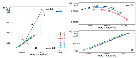
Figure 5.
QTAIM-DFA plots (Hb(rc) versus Hb(rc) − Vb(rc)/2) for the interactions in Br10 (Cs-L4), evaluated with MP2/6-311+G(3df); (a) whole region, (b) pure CS region, and (c) SS region. Marks and colors are shown in the figure.
QTAIM-DFA parameters of (R, θ) and (θp, κp) are obtained by analyzing the plots of Hb(rc) versus Hb(rc) − Vb(rc)/2, according to Equations (S3)–(S6). Table 1 collects the QTAIM-DFA parameters for the noncovalent Br-∗-Br interactions of Br4 (Cs-L1)–Br12 (Cs-L5), Br6 (C2), and Br10 (C2) together with the Cii values. Table 2 collects the (R, θ) and (θp, κp) values for Br4–Br12, other than those given in Table 1, together with the Cii values. The (R, θ) and (θp, κp) values for the covalent Br-∗-Br bonds in Br4–Br12 are collected in Table S4.
3.4. The Nature of Br-∗-Br Interactions in Polybromine Clusters
The nature of the covalent and noncovalent Br-∗-Br interactions in Br2–Br12 is discussed on the basis of the (R, θ, θp) values, employing standard values as a reference (see Scheme SA3).
It is instructive to survey the criteria shown in Scheme SA3 before detailed discussion. The criteria tell us that 180° < θ (Hb(rc) − Vb(rc)/2 < 0) for the SS interactions and θ < 180° (Hb(rc) − Vb(rc)/2 > 0) for the CS interactions. The CS interactions are subdivided into pure CS interactions (p-CS) of 45° < θ < 90° (Hb(rc) > 0) and regular CS interactions (r-CS) of 90° < θ < 180° (Hb(rc) < 0). The θp value predicts the character of interactions. In the pure CS region of 45° < θ < 90°, the character of interactions will be the vdW type for 45° < θp < 90° and the typical-HB type with no covalency (t-HBnc) for 90° < θp < 125°, where θp = 125° approximately corresponds to θ = 90°. The classical chemical covalent bonds of SS (180° < θ) will be strong when R > 0.15 au (Cov-s: strong covalent bonds), whereas they will be weak for R < 0.15 au (Cov-w: weak covalent bonds).
The (R, θ, θp) values are (0.0576 au, 184.3°, 190.9°) for the original Br2 if evaluated with MP2/6-311+G(3df). Therefore, the nature of the Br-∗-Br bond in Br2 is classified by the SS interactions (θ > 180°) and characterized to have a Cov-w nature (θp > 180° and R < 0.15 au). The nature is denoted by SS/Cov-w. The (R, θ, θp) values for the covalent Br-∗-Br bonds in Br4–Br12 are (0.0472–0.0578 au, 182.0–184.4°, 190.4–192.1°); therefore, their nature is predicted to be SS/Cov-w. The nature of the covalent Br-∗-Br bonds seems unchanged in the formation of the clusters [53,54]. The noncovalent Br-∗-Br interactions in Br4–Br12 are all classified by pure CS interactions since θ ≤ 76° (<< 90°) [53,54]. The θp values in the Cs-Lm clusters change systematically. The θp values for r2 in Br2k (Cs-Lm) (k = 2–6) are predicted to be in the range of 89.1° ≤ θp ≤ 89.6°, with θp = 87.9° for Br4 (Cs-L1).
However, the values for rn-2 in Br2k (Cs-Lm) (k = 2–6) are in the range of 90.6° ≤ θp ≤ 91.2° and the values for noncovalent interactions, other than edge positions, are in the range of 92.1° ≤ θp ≤ 93.0°. Namely, the noncovalent Br-∗-Br interactions are predicted to have the vdW nature (p-CS/vdW) for r2, while the interactions other than r2 are predicted to have the t-HBnc nature (p-CS/t-HBnc) since θp > 90°. The θp values of r2 for the Cs-Lm clusters will be less than 90°, irrespective of the angles between r1 and r2, which are close to 180°. The θp values will be larger than 90° for all noncovalent interactions other than r2. Table 1 contains the data for Br10 (C2), of which θp = 90.4° (> 90°) for r2 and θp = 87.1° (<90°) for r4, although Br10 (C2) is not the Cs-Lm type. The results for r2 seem reasonable based on the structure (cf. Figure 3), while those for r4 would be complex. Table 1 summarizes the predicted nature.
In the case of the noncovalent Br-∗-Br interactions in Br4–Br12, other than the Cs-Lm type clusters, θp > 90° for r2 in Br8 (S4) (θp = 93.4°) and Br8 (S4-Wm) (θp = 94.8°) and for r2, r4, and r6 in Br12 (Ci) (93.4° ≤ θp ≤ 93.7°). The interactions would have the t-HBnc nature (p-CS/t-HBnc). Very weak noncovalent Br-∗-Br interactions are also detected. The ranges of 64.2° ≤ θ ≤ 66.6° and 66.2° ≤ θp ≤ 71.2° are predicted for r2 and r3 in Br4 (C2h), r2 in Br4 (C2v), r3 in Br8 (S4-Wm), and r7 and r8 in Br10 (C2-c). The results are summarized in Table 2.
What are the relationships between the QTAIM-DFA parameters for the noncovalent Br-∗-Br interactions? The θ and θp values are plotted versus R. The plots are shown in Figure S4; they give very good correlations. The θp values are plotted versus θ. The plot is shown in Figure S5; it also gives a very good correlation. Table 3 summarizes the correlations among the QTAIM-DFA parameters.
Table 3.
Correlations in the plots 1.
To further examine the behavior of noncovalent Br-∗-Br interactions, NBO analysis is applied to the interactions.
3.5. NBO Analysis for Br-∗-Br of Br4 (Cs-L1)–Br12 (Cs-L5)
The noncovalent Br-∗-Br interactions in Br4(Cs-L1)–Br12 (Cs-L5) are characterized by σ(3c–4e) of the n(Br)→σ*(Br–Br) type. NBO analysis [56] was applied to the n(Br)→σ*(Br–Br) interactions with MP2/6-311+G(3df). For each donor NBO (i) and acceptor NBO (j), the stabilization energy E(2) is calculated based on the second-order perturbation theory in NBO. The E(2) values are calculated according to Equation (4), where qi is the donor orbital occupancy, εi, εj are diagonal elements (orbital energies), and F(i,j) is the off-diagonal NBO Fock matrix element. The values are obtained separately by the contributions from ns(Br)→σ*(Br–Br) and np(Br)→σ*(Br–Br), which are summarized in Table S5. The total values corresponding to ns+p(Br)→σ*(Br–Br) (=ns(Br)→σ*(Br–Br) + np(Br)→σ*(Br–Br)) were calculated, which are also summarized in Table S5. The total values are employed for the discussion.
E(2) = qi × F(i,j)2/(εj − εi)
Figure 6 shows the plots of E(2) and θp for the noncovalent Br-∗-Br interactions in Br4 (Cs-L1)–Br12 (Cs-L5). The values become larger in the order of P (r2: Br4 (Cs-L1)) < P (r2: Br6 (Cs-L2)–Br12 (Cs-L5)) < P (rω: Br6 (Cs-L2)–Br12 (Cs-L5)) < P (rin: Br6 (Cs-L2)–Br12 (Cs-L5)), where P means E(2) or θp, while rω and rin stand for the last end and the inside noncovalent interactions, respectively, in the sequence (see Figure 2 and Figure 3). The values for P = E(2) are as follows: E(2) = 16.6 kJ mol−1 for r2 in Br4 (Cs-L1) < 17.7 ≤ E(2) ≤ 18.2 kJ mol−1 for r2 in Br6 (Cs-L2)–Br12 (Cs-L5) < 19.5 ≤ E(2) ≤ 20.0 kJ mol−1 for rω in Br6 (Cs-L2)– Br12 (Cs-L5) < 21.2 ≤ E(2) ≤ 22.0 kJ mol−1 for rin in Br8 (Cs-L3)–Br12 (Cs-L5).
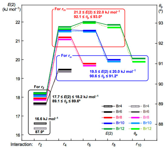
Figure 6.
Plots of θp and E(2) for the noncovalent Br-∗-Br interactions in Br4 (Cs-L1)–Br12 (Cs-L5). Colors are shown in the figure.
Relations between E(2) and Cii were also examined for noncovalent Br-∗-Br interactions in Br4 (Cs-L1)–Br12 (Cs-L5). The E(2) values were plotted versus Cii−1 for the noncovalent interactions. Figure 7 shows the plot. The plot gives a very good correlation, which is shown in Table 3 (Entry 5). The results show that the energies for σ(3c–4e) of the np(Br)→σ*(Br–Br) type in Br4 (Cs-L1)–Br12 (Cs-L5) are well evaluated, not only by E(2) but also by Cii−1. Similar relations would be essentially observed for the interactions in the nonlinear clusters; however, the analyses will be much complex due to the unsuitable structures for the NBO analysis, such as the deviations in the interaction angles expected for Br3 σ(3c–4e), the mutual interactions between Br3 σ(3c–4e), and/or the steric effect from other bonds and interactions, placed proximity in space. The E(2) values for Br4 (Cs-L1)–Br12 (Cs-L5) were also plotted versus R, θ, and θp, shown in Figures S6–S8, respectively. The plots give very good correlations, which are given in Table 3 (Entries 6–8).
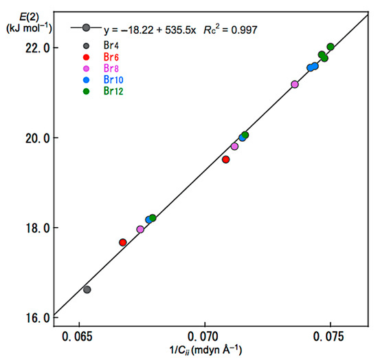
Figure 7.
Plot of E(2) versus 1/Cii for the noncovalent Br-∗-Br interactions in Br4 (Cs-L1)–Br12 (Cs-L5).
3.6. MO Descriptions for Noncovalent Br-∗-Br Interactions in Br4
As discussed above, Br3 σ(3c–4e) of the np(Br)→σ*(Br–Br) type plays an important role in the formation of Br4 (Cs-L1)–Br12 (Cs-L5). However, there must exist some interactions, other than Br3 σ(3c–4e), to stabilize the clusters. The ΔEES values for Br4 (C2h) (−8.0 kJ mol−1) and Br4 (D2d) (−9.1 kJ mol−1) are not so different from that for Br4 (Cs-L1) (−10.7 kJ mol−1). However, Br4 (C2h) and Br4 (D2d) must consist of interactions other than σ(3c–4e). Indeed, Br3 σ(3c–4e) of the n(Br)→σ*(Br–Br) type contributes to stabilizing Br4 (Cs-L1), but Br4 (C2h) and Br4 (D2d) are shown to be stabilized by the σ(Br–Br)→σ*Ry(Br) interaction by NBO, where Ry stands for the Rydberg term, although not shown.
The total energy for a species (E) is given by the sum of the core terms (Hc(i)) over all electrons, Σin Hc(i), and the electron–electron repulsive terms, (Σi≠jn Jij − Σi≠j,‖n Kij)/2, as shown by Equation (5), where Hc(i) consists of the kinetic energy and electron–nuclear attractive terms for electron i. E contains the nuclear–nuclear repulsive terms, although not clearly shown in Equation (5). As shown in Equation (6), the sum of MO energy for electron i, εi, over all electrons, Σi=1n εi, will be larger than E by (Σi≠jn Jij − Σi≠j,‖n Kij)/2 since the electron–electron repulsions are doubly counted in Equation (6). Therefore, Σin Hc(i) and (Σi≠jn Jij − Σi≠j,‖n Kij)/2 are given separately by Equations (7) and (8), respectively. The εi values for Br4 (C2h), Br4 (D2d), and 2Br2, together with Br4 (Cs-L1), are collected in Tables S6–S9, respectively, for convenience of discussion. Parameters (ΔP) in the formation of Br2k from the components are evaluated according to Equation (9). The ΔΣin Hc(i) and Δ(Σi≠jn Jij − Σi≠j,‖n Kij)/2 values for the formation of Br4 (C2h), Br4 (D2d), and Br4 (Cs-L1) are collected in Table S11.
E = Σin Hc(i) + (Σi≠jn Jij − Σi≠j,‖n Kij)/2
Σi=1n εi = Σin Hc(i) + (Σi≠jn Jij − Σi≠j,‖n Kij)
Σin Hc(i) = 2E − Σi=1n εi
(Σi≠jn Jij − Σi≠j,‖n Kij)/2 = Σi=1n εi − E
ΔP(Br2k) = P(Br2k) − kP(Br2)
The nature of noncovalent Br---Br interactions in Br4 (Cs-L1) is examined first. The σ(3c–4e) character in Br4 (Cs-L1) is confirmed by the natural charge evaluated with NPA (Qn), developed in the formation of Br4 (Cs-L1). The evaluated Qn values are Br(1: −0.0128|e−|)–Br(2: −0.0002|e−|)---Br(3: −0.0010|e−|)–Br(4: 0.0140|e−|); therefore, Qn(Br(4)–Br(3)) and Qn(Br(2)–Br(1)) are +0.013|e−| and −0.013|e−|, respectively. Each MO in Br4 (Cs-L1) is almost localized on Br(4)–Br(3) or Br(2)–Br(1), except for a few cases. MOs in Br4 (Cs-L1) must be affected by the local charge. Each MO energy in Br4 (Cs-L1) seems higher than the corresponding value of 2Br2 by 10–20 kJ mol−1 if the MO is localized on Br(2)–Br(1), lower by 15–25 kJ mol−1 on Br(3)–Br(4), and slightly lower by 0–5 kJ mol−1 if the MO is localized on the whole molecule. We should be careful since it depends on the phase in MO and the position of the Br atom(s). Typical cases are shown in Figure S9. In total, ΔΣi=1n εi is evaluated to be −357.2 kJ mol−1 for Br4 (Cs-L1). The results show that Br4 (Cs-L1) is stabilized in the formation of the dimer from the components through the lowering of MO energies in total, which is consistent with those evaluated with NBO, as discussed above.
Figure 8 shows the plots of ΔΣin Hc(i) and Δ(Σi≠jn Jij − Σi≠j,‖n Kij)/2 for Br4 (Cs-L1), Br4 (C2h), and Br4 (D2d), together with ΔEES and ΔΣi=1n εi. In the case of Br4 (Cs-L1), ΔΣin Hc(i) and Δ(Σi≠jn Jij − Σi≠j,‖n Kij)/2 are evaluated to be 335.7 and −346.4 kJ mol−1, respectively, which stabilizes Br4 (Cs-L1) in total. Two Br2 molecules in Br4 (Cs-L1) will supply a wider area for electrons without severe disadvantageous steric compression by the L-shaped structure in a plane. The structural feature of Br4 (Cs-L1) may reduce (or may not severely increase) the electron–electron repulsive terms, Δ((Σi≠jn Jij − Σi≠j,‖n Kij)/2), relative to the case of 2Br2, although ΔΣin Hc(i) seems to destabilize it. The ΔΣin Hc(i) + Δ(Σi≠jn Jij − Σi≠j,‖n Kij)/2 value is equal to −10.7 kJ mol−1, which corresponds to the stabilization energy of Br4 (Cs-L1), relative to 2Br2.
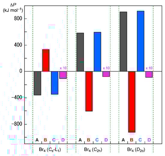
Figure 8.
Contributions from ΔΣinHc(i) (=ΔP = B) and Δ(Σi≠jn Jij − Σi≠j,‖n Kij)/2 (=ΔP = C) to ΔEES (=ΔP = D, magnified by 10 times in the plot) for Br4 (Cs-L1), Br4 (C2h), and Br4 (D2d), relative to 2Br2, together with ΔΣi=1n εi (=ΔP = A).
The energy profiles of Br4 (C2h) and Br4 (D2d) seem very different from that of Br4 (Cs-L1). The ΔΣi=1n εi terms for Br4 (C2h) and Br4 (D2d) are evaluated to be 587.5 and 908.1 kJ mol−1, respectively. Namely, Br4 (C2h) and Br4 (D2d) would be less stable than 2Br2 if ΔΣi=1n εi are compared. Consequently, it is difficult to explain the stability of Br4 (C2h) and Br4 (D2d), based on the MO energies. On the other hand, ΔΣin Hc(i) of Br4 (C2h) and Br4 (D2d) are evaluated to be −603.5 and −926.3 kJ mol−1, respectively, whereas Δ(Σi≠jn Jij − Σi≠j,‖n Kij)/2 are 595.5 and 917.2 kJ mol−1, respectively. As a result, the (ΔΣin Hc(i) + Δ(Σi≠jn Jij − Σi≠j,‖n Kij)/2) values are −8.0 and −9.1 kJ mol−1 for Br4 (C2h) and Br4 (D2d), respectively, which correspond to their ΔEES values (relative to 2E(Br2)). The results show that the stabilizing effect of ΔΣin Hc(i) overcomes the shorter electron–nuclear distances in the species on average. The shorter electron–electron distances must destabilize Br4 (C2h) and Br4 (D2d) through the factor of Δ(Σi≠jn Jij − Σi≠j,‖n Kij)/2, which is the inverse effect from the electron–nuclear interaction on ΔΣin Hc(i). However, the effect of the shorter distances on ΔΣin Hc(i) seems to contribute more effectively than the case of Δ(Σi≠jn Jij − Σi≠j,‖n Kij)/2 in Br4 (C2h) and Br4 (D2d), although they are not so large.
How can the BPs in Br4 (C2h) and Br4 (D2d) be rationalized through orbital interactions? The Δεi values of Br4 (C2h) are positive for all occupied MOs, relative to the corresponding values of 2Br2, except for HOMO-3 (−5.5 kJ mol−1), HOMO-6 (−2.9 kJ mol−1), HOMO-7 (−35.8 kJ mol−1), and HOMO-13 (−1.1 kJ mol−1). Figure 9 illustrates the interactions to produce HOMO, HOMO-3, HOMO-4, and HOMO-7. Indeed, HOMO-7 seems to contribute well to stabilizing Br4 (C2h), but HOMO-4 (+40.8 kJ mol−1) is also formed in the π(Br2)–π(Br2) mode. Similarly, HOMO (+13.7 kJ mol−1) is formed, together with HOMO-3 in the π*(Br2) + π*(Br2) mode. Therefore, all MOs seem not to contribute to stabilizing Br4 (C2h) inherently. Nevertheless, HOMO, HOMO-4, and HOMO-7 seem to rationalize the appearance of BPs in Br4 (C2h), along the diagonal line and shorter sides of the parallelogram, although all electrons contribute to the appearance of BPs in molecules.
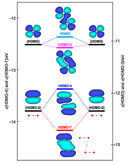
Figure 9.
Energy profile for the formation of Br4 (C2h), exemplified by HOMO, HOMO-3, HOMO-4, and HOMO-7.
Similarly, Δεi of Br4 (D2d) are positive for all occupied MOs, relative to the corresponding values of 2Br2, except for HOMO-3 (−1.9 kJ mol−1), HOMO-7 (−39.2 kJ mol−1), and HOMO-13 (−0.5 kJ mol−1). Figure 10 illustrates the interactions to produce HOMO, HOMO-3, HOMO-4, and HOMO-7 in Br4 (D2d). HOMO-4 (+50.2 kJ mol−1) is formed through the π(Br2)–π(Br2) mode in addition to HOMO-7. Similarly, HOMO (+13.9 kJ mol−1) is formed, accompanied by HOMO-3, in the π*(Br2) + π*(Br2) mode. Therefore, no MOs essentially stabilize Br4 (D2d). However, the appearance of BPs along the longer and shorter diagonal lines of the tetrahedron of Br4 (D2d) seem to be rationalized by HOMO-7, together with HOMO-3 and HOMO-4, modifying the BPs, although BPs will appear as the whole properties of molecules.
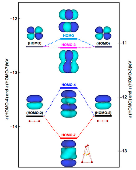
Figure 10.
Energy profile for the formation of Br4 (D2d), exemplified by HOMO, HOMO-3, HOMO-4, and HOMO-7.
The nature of interactions in the charged clusters is also of interest. Such investigations are in progress.
4. Conclusions
The intrinsic dynamic and static nature of noncovalent Br-∗-Br interactions was elucidated for Br4–Br10 with MP2/6-311+G(3df). QTAIM-DFA was applied to the investigation. Hb(rc) were plotted versus Hb(rc) − Vb(rc)/2 for the interactions at BCPs of the fully optimized structures, together with those from the perturbed structures, generated with CIV. The nature of the covalent Br-∗-Br bonds in Br4–Br10 is predicted to have the SS/Cov-w nature if calculated with MP2/6-311+G(3df). On the other hand, the nature of the noncovalent Br-∗-Br interactions in Br4–Br12 is classified by the pure CS interactions (θ ≤ 76°). The noncovalent Br-∗-Br interactions in the linear type clusters of Br4 (Cs-L1)–Br12 (Cs-L5) are predicted to have the p-CS/t-HBnc nature (90.6° ≤ θp), except for r2, outside the ones of the first end, which have the p-CS/vdW nature, although it is very close to the border area between the two (θp ≤ 89.4°). In the case of the cyclic clusters, the noncovalent Br-∗-Br interactions will have the p-CS/vdW nature (θp ≤ 88.4°), except for r2 in Br8 (S4) (θp = 93.5°) and Br8 (S4-Wm) (θp = 95.3°), which have the p-CS/t-HBnc nature.
The energies for Br3 σ(3c–4e) of the np(Br)→σ*(Br–Br) type are well evaluated by not only E(2) but also Cii−1 for Br4 (Cs-L1)–Br12 (Cs-L5). E(2) correlates very well to Cii−1. The CT interactions of the np(Br)→σ*(Br–Br) type must contribute to form Br4 (Cs-L1), which can be explained based on the MO energies, εi. However, it seems difficult to explain the stability of Br4 (C2h) and Br4 (D2d) based on the energies. The Br2 molecules must be stacked more effectively in Br4 (C2h) and Br4 (D2d), resulting in shorter electronuclear distances on average. The energy lowering effect by ΔΣin Hc(i), due to the effective stacking of 2Br2 in Br4 (C2h) and Br4 (D2d), contributes to form the clusters, although the inverse contribution from Δ((Σi≠jn Jij − Σi≠j,‖n Kij)/2) must also be considered.
Supplementary Materials
The following are available online, Table S1: Structural parameters for Br2–Br6, Table S2: Structural parameters for Br8–Br12, Table S3: The bond path distances and the straight-line distances in the polybromide clusters, together with the differences between the two, Table S4: The ρb(rc), Hb(rc) − Vb(rc)/2 (=(ћ2/8m)∇2ρb(rc)), and Hb(rc) values and QTAIM-DFA parameters for Br-∗-Br in polybromine clusters of Br2–Br12, Table S5: Contributions from the donor–acceptor (NBO(i)→NBO(j)) interactions of the n(Br)→σ*(Br–Br) type in the optimized structures of Br4–Br12, calculated using NBO analysis, Table S6: MO energies of Br4 (C2h), Table S7: MO energies of Br4 (D2d), Table S8: MO energies of Br2 (D∞h), Table S9: MO energies of Br4 (Cs-L1), Table S10: The Δεi values for Br4 (Cs-L1), relative to 2Br2 (D∞h), Table S11: Energies for the Br4 clusters and 2Br2, together with the differences between the two, Figure S1: Plot of ΔEZP versus ΔEES for Br4–Br12, relative to those of Br2, respectively, Figure S2: Plots of ΔEES for Br2–Br12 (Cs-Ln), Figure S3: Optimized structures for the cyclic bromine clusters of Br8–Br12, together with the linear type bromine cluster of Br10, Figure S4: Plot of θ and θp versus R for the noncovalent Br-∗-Br interactions at the BCPs in the fully optimized structures of Br4–Br12, Figure S5: Plot of θp versus θ for the noncovalent Br-∗-Br interactions at the BCPs in the fully optimized structures of Br4–Br12, Figure S6: Plot of E(2) versus R for noncovalent Br-∗-Br interactions in Br4 (Cs-L1)–Br12 (Cs-L5), Figure S7: Plot of E(2) versus θ for noncovalent Br-∗-Br interactions in Br4 (Cs-L1)–Br12 (Cs-L5), Figure S8: Plot of E(2) versus θp for noncovalent Br-∗-Br interactions in Br4 (Cs-L1)–Br12 (Cs-L5), Figure S9: MOi (i = 70, 67, 64, 35, and 30) and the energies relative to those corresponding to 2Br2, and Cartesian coordinates and energies of all the species involved in the present work. Appendix: Survey of QTAIM, closely related to QTAIM dual-functional analysis; Criteria for classification of interactions: behavior of typical interactions elucidated by QTAIM-DFA; Characterization of interactions.
Author Contributions
S.H. and W.N. formulated the project. S.H., W.N., and T.N. optimized all compounds. T.N. and E.T. calculated the ρb(rc), Hb(rc) − Vb(rc)/2 (=(ћ2/8m)∇2ρb(rc)), and Hb(rc) values and evaluated the QTAIM-DFA parameters and analyzed the data. S.H. and W.N. wrote the paper, while T.N. and E.T. organized the data to assist the writing. All authors have read and agreed to the published version of the manuscript.
Funding
Japan Society for the Promotion of Science, Grant Number 17K05785.
Data Availability Statement
Data are contained within the article or Supplementary Materials.
Acknowledgments
This work was partially supported by a Grant-in-Aid for Scientific Research (No. 26410050) from the Ministry of Education, Culture, Sports, Science, and Technology of Japan. Theoretical calculations were partially performed at the Research Centre for Computational Science, Okazaki, Japan.
Conflicts of Interest
The authors declare no conflict of interest.
References and Notes
- Colin, J.J. Sur Quelques Combinaisons de l’Iode. Ann. Chim. 1814, 91, 252–272. [Google Scholar]
- Cavallo, G.; Metrangolo, P.; Pilati, T.; Resnati, G.; Terraneo, G. Halogen Bond: A Long Overlooked Interaction. In Halogen Bonding I: Impact on Materials Chemistry and Life Sciences (Topics in Current Chemistry); Metrangolo, P., Resnati, G., Eds.; Springer: New York, NY, USA, 2015; Chapter 1; pp. 1–18. [Google Scholar]
- Cavallo, G.; Metrangolo, P.; Milani, R.; Pilati, T.; Priimagi, A.; Resnati, G.; Terraneo, G. The Halogen Bond. Chem. Rev. 2016, 116, 2478–2601. [Google Scholar] [CrossRef]
- Bent, H.A. Structural chemistry of donor-acceptor interactions. Chem. Rev. 1968, 68, 587–648. [Google Scholar] [CrossRef]
- Desiraju, G.R.; Parthasarathy, R. The nature of halogen halogen interactions: Are short halogen contacts due to specific attractive forces or due to close packing of nonspherical atoms? J. Am. Chem. Soc. 1989, 111, 8725–8726. [Google Scholar] [CrossRef]
- Metrangolo, P.; Resnati, G. Halogen Bonding: A Paradigm in Supramolecular Chemistry. Chem. Eur. J. 2001, 7, 2511–2519. [Google Scholar] [CrossRef]
- Erdélyi, M. Halogen bonding in solution. Chem. Soc. Rev. 2012, 41, 3547–3557. [Google Scholar] [CrossRef]
- Beale, T.M.; Chudzinski, M.G.; Sarwar, M.G.; Taylor, M.S. Halogen bonding in solution: Thermodynamics and applications. Chem. Soc. Rev. 2013, 42, 1667–1680. [Google Scholar] [CrossRef] [PubMed]
- Legon, A.C. Prereactive Complexes of Dihalogens XY with Lewis Bases B in the Gas Phase: A Systematic Case for the Halogen Analogue B⋅⋅⋅XY of the Hydrogen Bond B HX. Angew. Chem. Int. Ed. 1999, 38, 2686–2714. [Google Scholar] [CrossRef]
- Politzer, P.; Murray, J.S.; Clark, T. Halogen bonding and other σ-hole interactions: A perspective. Phys. Chem. Chem. Phys. 2013, 15, 11178–11189. [Google Scholar] [CrossRef]
- Sugibayashi, Y.; Hayashi, S.; Nakanishi, W. Behavior of Halogen Bonds of the Y–X···Type (X, Y=F, Cl, Br, I) in the Benzene p System, Elucidated by Using a Quantum Theory of Atoms in Molecules Dual-Functional Analysis. Chem. Phys. Chem. 2016, 17, 2579–2589. [Google Scholar] [CrossRef] [PubMed]
- Desiraju, G.R.; Ho, P.S.; Kloo, L.; Legon, A.C.; Marquardt, R.; Metrangolo, P.; Politzer, P.; Resnati, G.; Rissanen, K. Definition of the halogen bond (IUPAC Recommendations 2013). Pure Appl. Chem. 2013, 85, 1711–1713. [Google Scholar] [CrossRef]
- Metrangolo, P.; Resnati, G. (Eds.) Halogen Bonding: Fundamentals and Applications; Series Structure and Bonding; Springer: New York, NY, USA, 2008. [Google Scholar]
- Gierszal, K.P.; Davis, J.G.; Hands, M.D.; Wilcox, D.S.; Slipchenko, L.V.; Ben-Amotz, D. π-Hydrogen Bonding in Liquid Water. J. Phys. Chem. Lett. 2011, 2, 2930–2933. [Google Scholar] [CrossRef]
- Categorizing Halogen Bonding and other Noncovalent Interactions Involving Halogen Atoms. a satellite event of the XXII Congress and General Assembly of the International Union of Crystallography, 2010; https://doi.org/10.1515/ci.2010.32.2.20 (accessed on 1 May 2021).
- Donohue, J.; Goodman, S.H. Interatomic distances in solid chlorine. Acta Cryst. 1965, 18, 568–569. [Google Scholar] [CrossRef]
- Powell, B.M.; Heal, K.M.; Torrie, B.H. The temperature dependence of the crystal structures of the solid halogens, bromine and chlorine. Mol. Phys. 1984, 53, 929. [Google Scholar] [CrossRef]
- Van Bolhuis, F.; Koster, P.B.; Migchelsen, T. Refinement of the crystal structure of iodine at 110° K. Acta Cryst. 1967, 23, 90–91. [Google Scholar] [CrossRef]
- Schuster, P.; Mikosch, H.; Bauer, G. All electron density functional study of neutral and ionic polybromine clusters. J. Chem. Phys. 1998, 109, 1833–1844. [Google Scholar] [CrossRef]
- Sung, D.; Park, N.; Park, W.; Hong, S. Formation of polybromine anions and concurrent heavy hole doping in carbon nanotubes. Appl. Phys. Lett. 2007, 90, 093502. [Google Scholar] [CrossRef]
- Nakanishi, W.; Hayashi, S.; Narahara, K. Polar Coordinate Representation of Hb(rc) versus (ћ2/8m)∇2ρb(rc) at BCP in AIM Analysis: Classification and Evaluation of Weak to Strong Interactions. J. Phys. Chem. A 2009, 113, 10050–10057. [Google Scholar] [CrossRef]
- Nakanishi, W.; Hayashi, S. Atoms-in-Molecules Dual Functional Analysis of Weak to Strong Interactions. Curr. Org. Chem. 2010, 14, 181–197. [Google Scholar] [CrossRef]
- Nakanishi, W.; Hayashi, S. Dynamic Behaviors of Interactions: Application of Normal Coordinates of Internal Vibrations to AIM Dual Functional Analysis. J. Phys. Chem. A 2010, 114, 7423–7430. [Google Scholar] [CrossRef]
- Nakanishi, W.; Hayashi, S.; Matsuiwa, K.; Kitamoto, M. Applications of Normal Coordinates of Internal Vibrations to Generate Perturbed Structures: Dynamic Behavior of Weak to Strong Interactions Elucidated by Atoms-in-Molecules Dual Functional Analysis. Bull. Chem. Soc. Jpn. 2012, 85, 1293–1305. [Google Scholar] [CrossRef]
- Nakanishi, W.; Hayashi, S. Role of dG/dw and dV/dw in AIM Analysis: An Approach to the Nature of Weak to Strong Interactions. J. Phys. Chem. A 2013, 117, 1795–1803. [Google Scholar] [CrossRef] [PubMed]
- Bader, R.F.W. Atoms in Molecules. A Quantum Theory; Oxford University Press: Oxford, UK, 1990. [Google Scholar]
- Matta, C.F.; Boyd, R.J. An Introduction to the Quantum Theory of Atoms in Molecules. In The Quantum Theory of Atoms in Molecules: From Solid State to DNA and Drug Design; WILEY-VCH: Weinheim, Germany, 2007. [Google Scholar]
- Nakanishi, W.; Hayashi, S.; Nishide, T. Intrinsic dynamic and static nature of each HB in the multi-HBs between nucleobase pairs and its behavior, elucidated with QTAIM dual functional analysis and QC calculations. RSC Adv. 2020, 10, 24730–24742. [Google Scholar] [CrossRef]
- See also Figure 5 for the definition of (R, θ) and (θp, κp), exemplified by the r9 in Br10 (Cs-L5).
- Nakanishi, W.; Hayashi, S. Perturbed structures generated using coordinates derived from compliance constants in internal vibrations for QTAIM dual functional analysis: Intrinsic dynamic nature of interactions. Int. J. Quantum Chem. 2018, 118, e25590–e25591. [Google Scholar] [CrossRef]
- The basic concept for the compliance constants was introduced by Taylor and Pitzer, followed by Konkoli and Cremer.
- Taylor, W.T.; Pitzer, K.S. Vibrational frequencies of semirigid molecules: A general method and values for ethylbenzene. J. Res. Natl. Bur. Stand. 1947, 38, 1–17. [Google Scholar] [CrossRef]
- Konkoli, Z.; Cremer, D. A new way of analyzing vibrational spectra. I. Derivation of adiabatic internal modes. Int. J. Quantum Chem. 1998, 67, 1–9. [Google Scholar] [CrossRef]
- The Cij are defined as the partial second derivatives of the potential energy due to an external force, as shown in Equations (R1), where i and j refer to internal coordinates, and the external force components acting on the system fi and fj correspond to i and j, respectively.
- Cij = ∂2E/∂fi∂fj (R1).
- The Cij Values and the Coordinates Corresponding to Cii Were Calculated by Using the Compliance 3.0.2 Program Released by Grunenberg, J. and Brandhorst, K. Available online: http://www.oc.tu-bs.de/Grunenberg/compliance.html (accessed on 1 May 2021).
- Brandhorst, K.; Grunenberg, J. Efficient computation of compliance matrices in redundant internal coordinates from Cartesian Hessians for nonstationary points. J. Chem. Phys. 2010, 132, 184101. [Google Scholar] [CrossRef]
- Brandhorst, K.; Grunenberg, J. How strong is it? The interpretation of force and compliance constants as bond strength descriptors. Chem. Soc. Rev. 2008, 37, 1558–1567. [Google Scholar] [CrossRef] [PubMed]
- Grunenberg, J. III-defined concepts in chemistry: Rigid force constants vs. compliance constants as bond strength descriptors for the triple bond in diboryne. Chem. Sci. 2015, 6, 4086–4088. [Google Scholar] [CrossRef] [PubMed][Green Version]
- Frisch, M.J.; Trucks, G.W.; Schlegel, H.B.; Scuseria, G.E.; Robb, M.A.; Cheeseman, J.R.; Scalmani, G.; Barone, V.; Mennucci, B.; Petersson, G.A.; et al. Gaussian 09 (Revision D.01), Gaussian, Inc.: Wallingford, CT, USA, 2009.
- Binning, R.C.; Curtiss, L.A. Compact contracted basis sets for third-row atoms: Ga–Kr. J. Comput. Chem. 1990, 11, 1206–1216. [Google Scholar] [CrossRef]
- Curtiss, L.A.; McGrath, M.P.; Blaudeau, J.-P.; Davis, N.E.; Binning, R.C., Jr.; Radom, L. Extension of Gaussian-2 theory to molecules containing third-row atoms Ga–Kr. J. Chem. Phys. 1995, 103, 6104–6113. [Google Scholar] [CrossRef]
- McGrath, M.P.; Radom, L. Extension of Gaussian-1 (G1) theory to bromine-containing molecules. J. Chem. Phys. 1991, 94, 511–516. [Google Scholar] [CrossRef]
- Clark, T.; Chandrasekhar, J.; Spitznagel, G.W.; Schleyer, P.v.R. Efficient diffuse function-augmented basis sets for anion calculations. III. The 3-21+G basis set for first-row elements, Li–F. J. Comput. Chem. 1983, 4, 294–301. [Google Scholar] [CrossRef]
- Møller, C.; Plesset, M.S. Note on an Approximation Treatment for Many-Electron Systems. Phys. Rev. 1934, 46, 618–622. [Google Scholar] [CrossRef]
- Gauss, J. Effects of electron correlation in the calculation of nuclear magnetic resonance chemical shifts. J. Chem. Phys. 1993, 99, 3629–3643. [Google Scholar] [CrossRef]
- Gauss, J. Accurate Calculation of NMR Chemical Shifts. Ber. Bunsen-Ges. Phys. Chem. 1995, 99, 1001–1008. [Google Scholar] [CrossRef]
- Biegler-König, F.; Schönbohm, J. The AIM2000 Program (Version 2.0). Available online: http://www.aim2000.de (accessed on 1 May 2021).
- Biegler-König, F. Calculation of atomic integration data. J. Comput. Chem. 2000, 21, 1040–1048. [Google Scholar] [CrossRef]
- Keith, T.A. AIMAll (Version 17.11.14), TK Gristmill Software, Overland Park KS, USA. 2017. Available online: http://aim.tkgristmill.com (accessed on 1 May 2021).
- See Figure 3 for Br4–Br12 of the L-shaped clusters in the Cs symmetry, Br4 (Cs-L1)–Br12 (Cs-L5), and Figure 4 for Br6–Br12 of the cyclic bromine clusters.
- See also Entry 1 in Table 3. http://aim.tkgristmill.com/ (accessed on 1 May 2021).
- The Br–Br distance in Br2 was optimized to be 2.2806 Å with MP2/6-311+G(3df), which was very close to the observed distance in the gas phase (2.287 Å). However, the values are shorter than that determined by the X-ray crystallographic analysis (2.491 Å) by 0.210 Å. The non-covalent Br---Br distance is 3.251 Å in crystal, which is shorter than the sum of the van der Waals radii by 0.45 Å.
- Bondi, A. van der Waals Volumes and Radii. J. Phys. Chem. 1964, 68, 441–451. [Google Scholar] [CrossRef]
- The molecular graph for Br4 (C2h) was very complex and very different from that expected for it when calculated with MP2/6-311+G(3df)//MP2/6-311+G(3df). Some (ω,σ) = (3, −3) attractors appear in the molecular graph of Br4 (C2h), which do not correspond to bromine atoms. Therefore, the molecular graph for Br4 (C2h) were drawn with MP2/6-311+G(d)//MP2/6-311+G(3df), which was shown in Figure 2. The ρb(rc), Hb(rc) − Vb(rc)/2 (=(ћ2/8m)∇2ρb(rc)), and Hb(rc) values were calculated with the same method.
- Glendening, E.D.; Reed, A.E.; Carpenter, J.E.; Weinhold, F. NBO, Gaussian, Inc.: Pittsburgh, PA, USA, 2003; version 3.1.


Publisher’s Note: MDPI stays neutral with regard to jurisdictional claims in published maps and institutional affiliations. |
© 2021 by the authors. Licensee MDPI, Basel, Switzerland. This article is an open access article distributed under the terms and conditions of the Creative Commons Attribution (CC BY) license (https://creativecommons.org/licenses/by/4.0/).