1. Introduction
Mass spectrometry is one of the most powerful tools for pure substances’ identifications [
1]. The mass spectral data contains a sequence of mass/charge (
m/
z) ratios and their intensities. The substance qualitative analysis information, such as relative molecular weight determination, chemical formula determination, and structural identification, can be obtained by comparing the measured mass spectra with the standard mass spectra manually. The peak in the mass spectra represents the distribution of ions in samples. According to the resolution difference, the mass spectral data can be divided into two types: high resolution and low resolution [
2]. Low resolution mass spectra can only distinguish different nominal mass ions. High resolution mass spectra can calculate the precise mass for each ionized compound. Even isotopes can be distinguished by the high-resolution mass spectrometry. The presence of isotopes, as well as the sample purity, electronic noise, or the accuracy of mass spectrometers, will significantly affect the high-resolution mass spectral data [
3]. Even under such delicately experimental conditions controlling, it is hard to obtain the identical mass spectra.
However, in real life scenarios, different compounds are often mixed together. Because of the complication of mass spectra the mathematical methods were often utilized to detect the specified compounds in the mixing samples [
4]. Machine learning has been applied as an efficient tool in the analytical chemistry for a long time [
5]. Partial least squares (PLS) is one of the methods used for compound detection [
6]. However, when data is large-scale, PLS does not work well. Over the past several years, many works on artificial neural network (ANN) in the area of mass spectrometry have been reported [
7]. MSnet, created by Curry et al. might be the earliest general neural network used in mass spectra analysis [
8]. It involves a hierarchical system of several neural networks for mass spectrometry. Werther et al. compared the ANN performances using classical multidimensional numerical analysis techniques [
9]. A. Eghbaldar et al. presented a methodology for the optimization of ANN to identify the compounds’ structural features from mass spectral data [
10]. Ion mobility spectra could also be successfully classified by neural networks from the combination of drift time, number, intensity, and shape of peaks [
11].
In general, good performance of ANN is often based on the large-scale data sets. Furthermore, the large dimension of the mass spectra input data is a natural characteristic for the ‘‘data–response’’ correlation problems [
12]. Unfortunately, a small number of samples and the large dimension of inputs construct the typical dilemma for the real data sets. In analytical chemistry, principal component analysis (PCA), as a traditional method, is regularly applied for the dimension-reduction of data [
13]. Although PCA has a wide range of application areas such as data compression to eliminate redundancy and data noise cancellation. PCA can only obtain principal components in a single direction. The principal components with small contribution rates may often contain important information for sample dissimilarities. In some cases, these principal components cannot be ignored. Because of the complexity and the size of the mass spectra data, automated feature extraction is frequently required to process the data [
14]. Continuous wavelet transform (CWT) shows a better best performance among several peak detection algorithms for the mass spectra data [
15]. Deep learning, by neural unit learning data characteristics, can extract features from raw large dimension data directly [
16]. Deep learning was explored to predict molecular substructure in the mass spectral data [
17]. Because the deep neural network (DNN) is not suitable for the time series data, the long short-term memory (LSTM)-based substance classification system was proposed for substance detections [
18]. Nevertheless, it is still difficult to detect a class with similar molecular structure inside the mixing sample mass spectra. Felicity Allen et al. built a web server for spectrum prediction and metabolite identification from tandem mass spectra based on deep learning [
19]. The multi-label classification can study each example associated with a set of labels simultaneously [
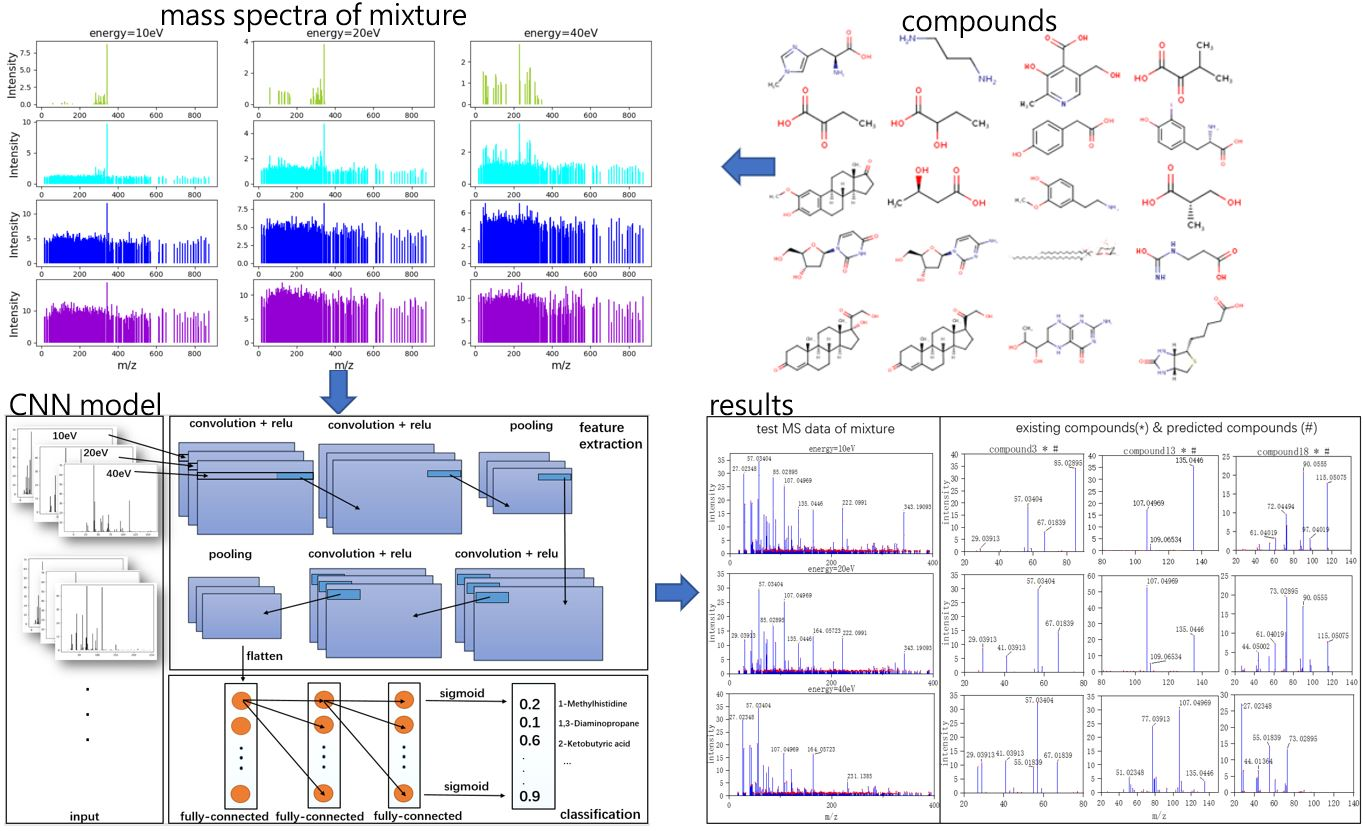
20]. In this paper, we analyzed the performance of multi-label classification techniques in the detection of the small molecule metabolites found in the human body within the samples. The pragmatic algorithm was based on convolutional neural networks (CNN). Boosting is a common machine learning method, which is widely used and effective. In classification problems, it improves the performance of classification by changing the weights of training samples, learning multiple classifiers, and linearly combining these classifiers. AdaBoost, GBDT, and XGBoost are the most classic algorithms of the Boosting series. We chose XGBoost for comparison, which performed best in this work among the three algorithms. Compared with other algorithms, CNN can separate independent mass spectra contributed by different compounds to achieve better accuracy. Imitating the CNN architecture, three-channel architecture [
21] has been used as input. Comparison with the traditional classification methods, the methodology can significantly enhance the predicting accuracy and performance for the mixing sample. Meanwhile, this model has a greater potential for large-target mass spectral data analysis.
2. Results
We have used the loss function to estimate the degree of inconsistency between the predicted value of the model and the true value. The smaller the loss function, the better is the robustness of the model. In the classification problem of machine learning, sigmoid and softmax are activation functions often used in the output layer of the neural network. They are functions used for binary and multi-class classification, but sigmoid can also be used for multi-class. The difference is that multiple classes in sigmoid may mutually overlap, softmax must be based on the premise of various types of mutual exclusion, and the sum of the probability of each category is one. Binary cross-entropy and categorical cross-entropy are the loss functions corresponding to sigmoid and softmax. In this work, sigmoid was employed as the activation function and the binary cross-entropy was employed as the loss function for multi-labels classification, which trains model fast and requires less memory:
where
x is the input sample,
m is the total number of training data,
y is the real label corresponding to the
ith category, and
f is the corresponding model output value.
Since the output of each label is assumed to be independent, the common configuration of multi-labels binary classification is BCE and sigmoid activation function. Each category output is a probability in the range of zero to one and corresponds to a sigmoid. Adam algorithm is used as the optimizer to iteratively update neural network weights based on the training data. The main advantage of Adam is that after the offset correction, each iteration learning rate has a certain range, which makes the parameters relatively stable. After 100 epochs of training, the accuracy, recall, and precision on the test set of each model for target compounds detection are shown in
Table 1.
As a result, all five machine learning models could achieve high accuracy for detecting multiple target compounds in the overlapping samples. It was indicated that they could learn features effectively from raw MS data directly. The results obtained by neural networks are often not labels such as zero or one, but they can obtain classification results such as 0.5, 0, 8. Therefore we should choose a threshold. When the result is more than the threshold, the predicted value is judged as one; when the result is less than or equal to threshold, the predicted value is judged as zero. Increasing the threshold, we will be more confident in the predicted value, which increases the precision. But this will reduce the recall. If the threshold is reduced, the number of true examples missed by the model will decrease, and the recall will increase. Here we chose 0.5 as a threshold. No matter how strong the noise was, CNN always achieved higher accuracy than the other two models. In fact, when average intensity of noise was 4 and variance is 0.8, most information of low intensity had been covered by noise. Because of good adaptive and outlier processing, CNN has the best performance of extracting features. Furthermore, for target compounds detection, the recall is the more important indicator. The recall reflects the correctly predicted components (true positive) accounts for the proportion of all components that should be predicted (true positive and true negative). Although it seems that the precision of PCA+SVM is not too low, the performance of PCA + SVM is much lower than neural networks. Because the PCA + SVM model predicts a large number of samples with positive labels as false (it does not detect the presence of compounds), it has much poorer recall performance than DNN and CNN. The precision of LSTM is high but the recall is low, it means the threshold should be reduced. XGBoost also seems to be a passable method. For further observation, we use the receiver operating characteristic (ROC) curve to evaluate the discriminative ability of the models [
22]. The comparison of the ROC curves (MS data with noise that average intensity is 1 and variance is 0.2) for five models is shown in
Figure 1.
Class 1: 1-methylhistidine; class 2: 1,3-diaminopropane; class 3: 2-ketobutyric acid; class 4: 2-hydroxybutyric acid; class 5: 2-methoxyestrone class 6: (R)-3-hydroxybutyric acid; class 7: deoxyuridine; class 8: deoxycytidine; class 9: cortexolone; class 10: deoxycorticosterone; class 11: 4-pyridoxic acid; class 12: alpha-ketoisovaleric acid; class 13: p-hydroxyphenylacetic acid; class 14: iodotyrosine; class 15: 3-methoxytyramine; class 16:(S)-3-hydroxyisobutyric acid; class 17: 3-O-sulfogalactosylceramide; class 18: ureidopropionic acid; class 19: tetrahydrobiopterin; class 20: biotin.
If the ROC curve was farther from the pure opportunity line (black dotted line), the model discrimination was stronger. Because of the mapping principle of the ROC curve, neural network methods and other methods have different curve shapes. According to
Figure 1, CNN has the largest average area under curve (AUC), and this means CNN has the best performance of classification. PCA + SVM has the least average AUC. At the same time, we can see that all classes have large AUC using CNN, but some classes have small AUC when using DNN, LSTM, and XGBoost. Hence, it can be concluded that CNN is the robust method in the five algorithms. The average precision (AP) score can also summarize the precision-recall curves as the weighted mean of precisions achieved at each threshold to estimate five models:
where
and
are the precision and recall at the
nth threshold. The AP can be considered as the fraction of positive samples. In multi-label classification, mean average precision (mAP) is a common evaluation measure:
where
is the average precision of the
nth label. Here mAP is equal to the area under average ROC curve.
Table 2 shows that PCA + SVM had poor classifier performance. Combining with
Table 1 and ROC curves in
Figure 1, CNN model has more stable performance of target detection for all compounds compared with DNN.
With interference data of 20 other compounds adding to mix with above simulate data (noise has 1 average intensity and 0.2 variance), the types and concentration of compounds would be random in the mixing samples.
Usually, metabolomic identification tasks may involve up to and over 100 metabolites. According to
Table 3 and
Table 4, when more metabolites are added, the accuracy reduction of CNN is smaller than other models. This shows that CNN is more feasible for large sample detection. Not only the 20 metabolites used in this work can be identified, more metabolites even other types of compounds can be classified using CNN.
3. Discussion
If more preprocesses such as smooth, baseline correction, and peak picking are applied to the data, the traditional machine learning algorithms such as SVM will perform better [
15]. Compared with traditional machine learning algorithms, deep learning does not need too much preprocessing or denoising. Good performance occurs in the single mass spectral data classification using SVM or deep learning [
23]. We can see the performance of the five models in
Table 5:
We used 600 MS data for the test. TP means all the compounds were detected; FP means part of the compounds were detected; TN means nonexistent compounds were predicted. In multi-label target detection of mixture mass spectral data, CNN performs better than SVM XGBoost, DNN, or LSTM. The result of test MS data demonstrates that CNN is the most promising model for multi-labels target detection of mixture MS data. In fact, SVM has a good effect on two-label classification problems. It does not work well in multi-label classification problems. Compared to DNN, CNN has better performance on mixture MS data. LSTM is more suitable for time series data analysis. In the case of large noise, the classification problem may appear to overfit using Boosting methods.
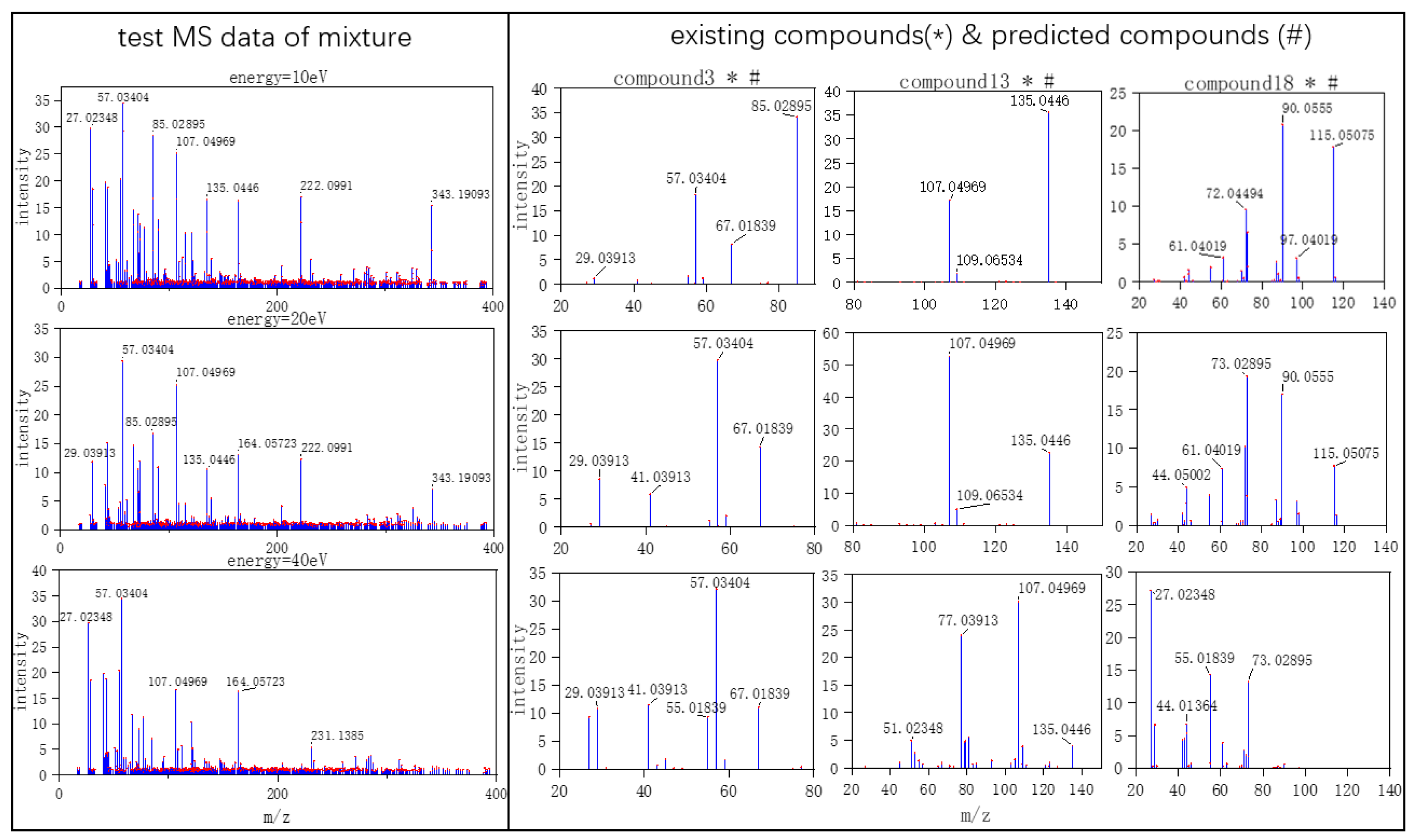
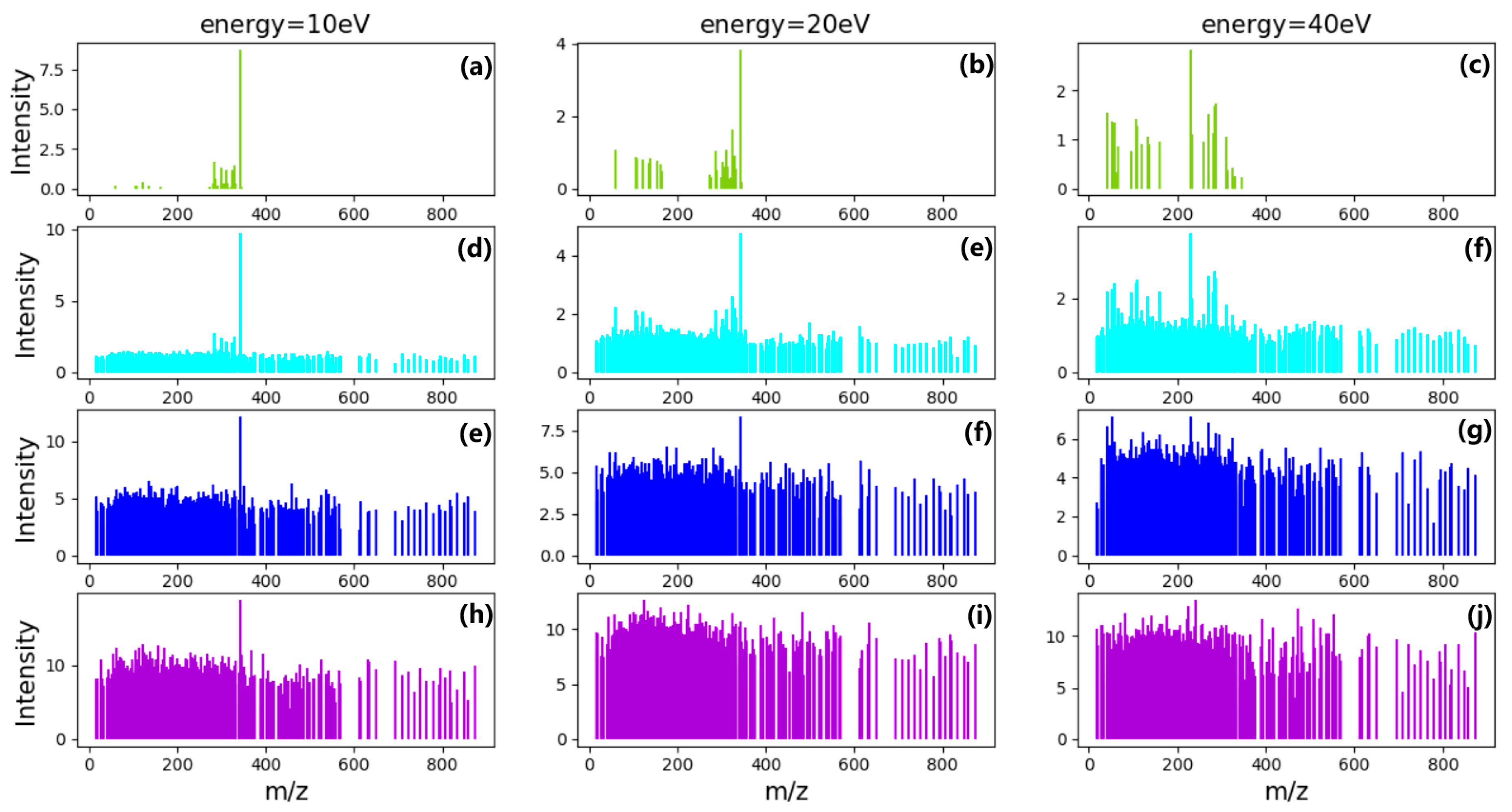
Three typical MS data were chosen to analyze the CNN model prediction. In
Figure 2,
Figure 3 and
Figure 4, on the left are the mass spectra of the mixture samples; on the right are the mass spectra of existing compounds in the mixture and the mass spectra of the predicted compounds. As shown in
Figure 2, MS data consists of compound 3, compound 13, compound 18 and all the compounds that have been detected. In
Figure 3, MS data consists of compound 4, compound 18, compound 15, and compound 16, but compound 4 missed in the prediction of the model, because the intensity of compound 4 is much weaker than the other three compounds. Compound 4 in this MS data is hard to be detected. In
Figure 4, MS data consists of compound 6, compound 8, compound 16, and compound 18. From observation, the intensity of compound 6 and compound 16 are smaller compared to compound 8. This caused the model to predict the presence of compound 6 erroneously.
As Skarysz et al. speculated, the increased performance of CNN might be due to the following reasons. 1. The convolution filter can allow the CNN to learn the peak shape, not just the same
m/
z axis. 2. Such filters allow for greater robustness before low signal to noise ratios. 3. The depth of CNN may allow for a higher-level representation of the low-level features characterizing each individual pattern [
23].
CNN is mainly used to identify two-dimensional graphics that are invariant to displacement, scaling, and other forms of distortion. The shape of each compound in mass spectra is similar to feature in graphics. Since the CNN feature detection layer learns from training data, explicit feature extraction is avoided, and learning is implicitly performed from the training data when using CNN. CNN has good ability to learn low-level features from complicated input. Meanwhile, CNN is less affected by noise because of the robustness of filters. If there is more MS data of different energy as input, CNN will learn more relationships between different energy. Once more MS data of different energy as input are added, even continuous signal in energy axis, further studies needed to be made to the architecture of CNN including depth, alternating layers, and filter sizes to improve the ability to learn and detect the target compounds. As an easier controllable variable factor, the energy was selected as one input channel instead of time.
The analysis of spectral data sets with small number samples is a bottleneck for deep learning including DNN, CNN, etc. Normally, those models require large data sets to learn the features of samples [
12]. For this reason, deep learning may not achieve good performance in target detection when spectral data sets are small. Based on the assumption of linear mixture model, adding simulation data into data set is a method to solve the problem of the training data shortage. When dealing with MS data with different noise in
Table 1, the mean average precision scores of SVM + PCA model are 0.72, 0.71, 0.68, and 0.62; the mAP scores of DNN are 0.96, 0.95, 0.92, and 0.88; the mAP scores of LSTM are 0.94, 0.92, 0.87, and 0.84; the mAP scores of XGBoost are 0.94, 0.93, 0.91, and 0.87. Meanwhile, the mAP scores of CNN are 0.99, 0.98, 0.95, and 0.92. When interference data were added, the mAP scores for the five models are 0.65, 0.80, 0.82, 0.84, and 0.95.
Compared with traditional algorithms, deep learning is more transferable and less affected by data. In real situations, owing to the differences in operator, instruments, and experimental environments, MS data may vary momentously. It is essential to control variable factor and obtain a large-scale data set for training models by data obtained under the same conditions and data expansion. Training model by input MS data from different instruments, adding more offset MS data will make models have stronger universality. Our established methodology could efficiently achieve the multiple compounds recognition from the tandem mass spectral data.


