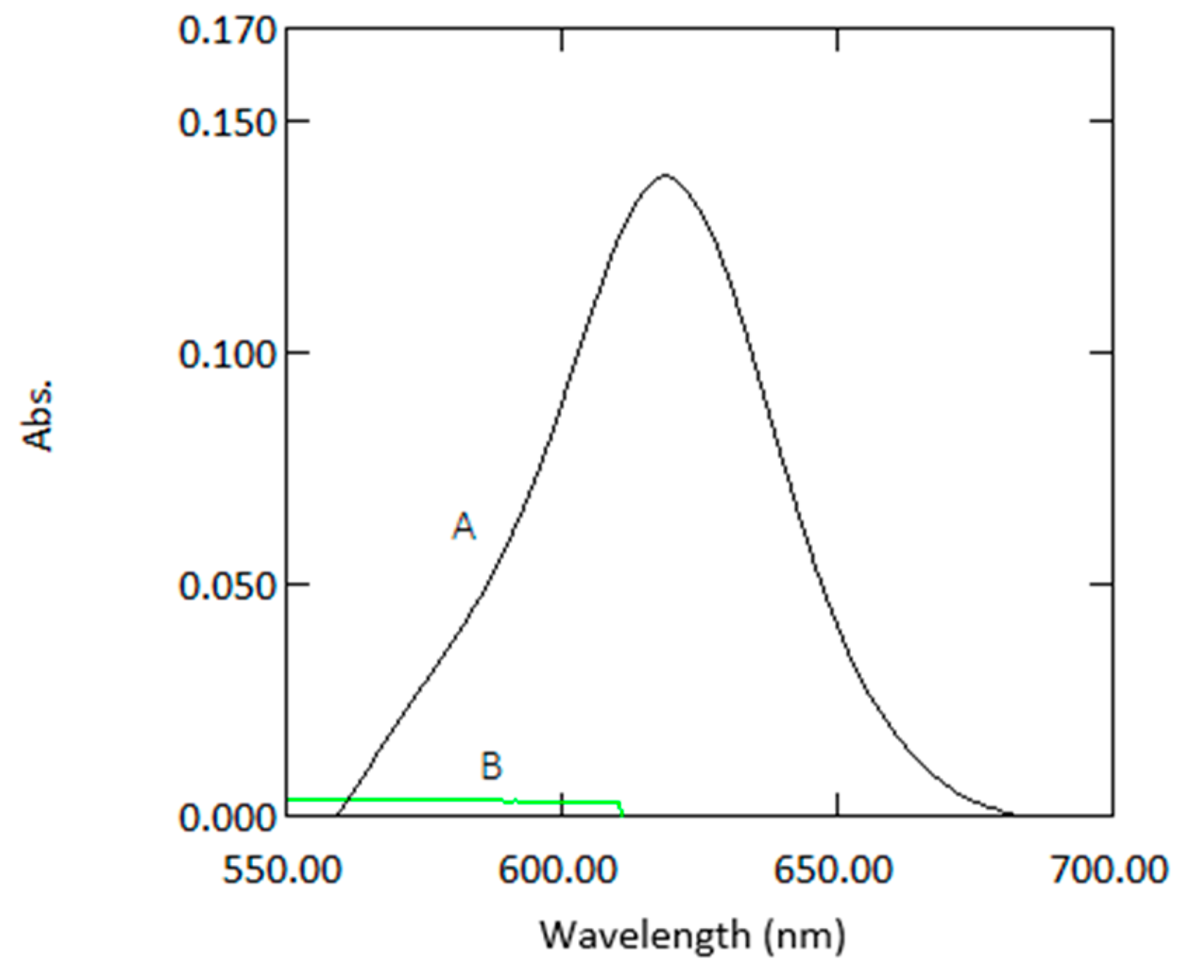
Figure 1.
Absorption spectra of coloured species (1 µg mL−1 arsenic) versus reagent blank (A) and reagent blank versus double deionized water (B).
Figure 1.
Absorption spectra of coloured species (1 µg mL−1 arsenic) versus reagent blank (A) and reagent blank versus double deionized water (B).
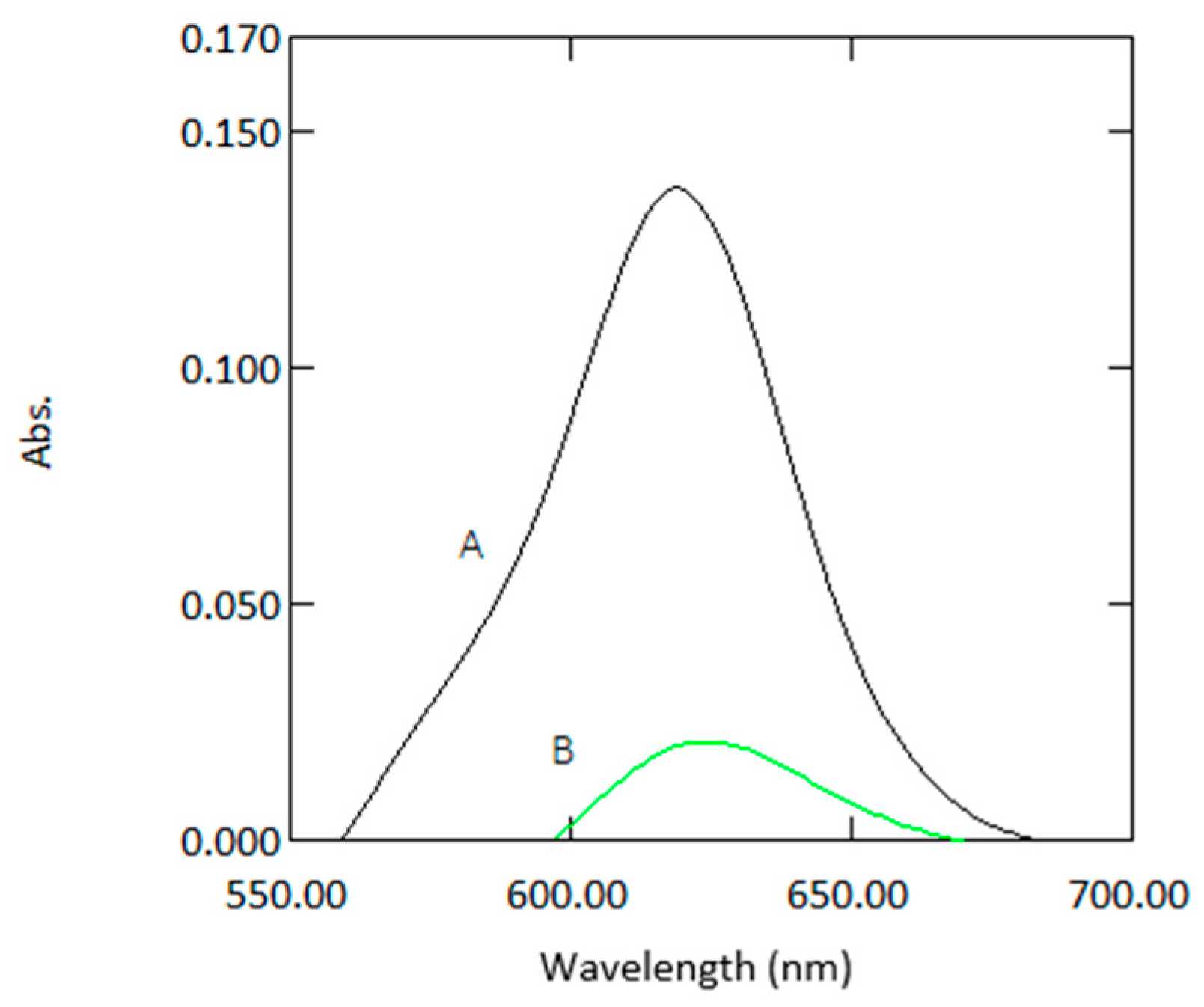
Figure 2.
Absorption spectra of a sample containing 1µg mL−1 arsenic with reagents measured in 10 mm cuvettes (A) and 1 mm quartz cuvettes (B) against reagent blank.
Figure 2.
Absorption spectra of a sample containing 1µg mL−1 arsenic with reagents measured in 10 mm cuvettes (A) and 1 mm quartz cuvettes (B) against reagent blank.
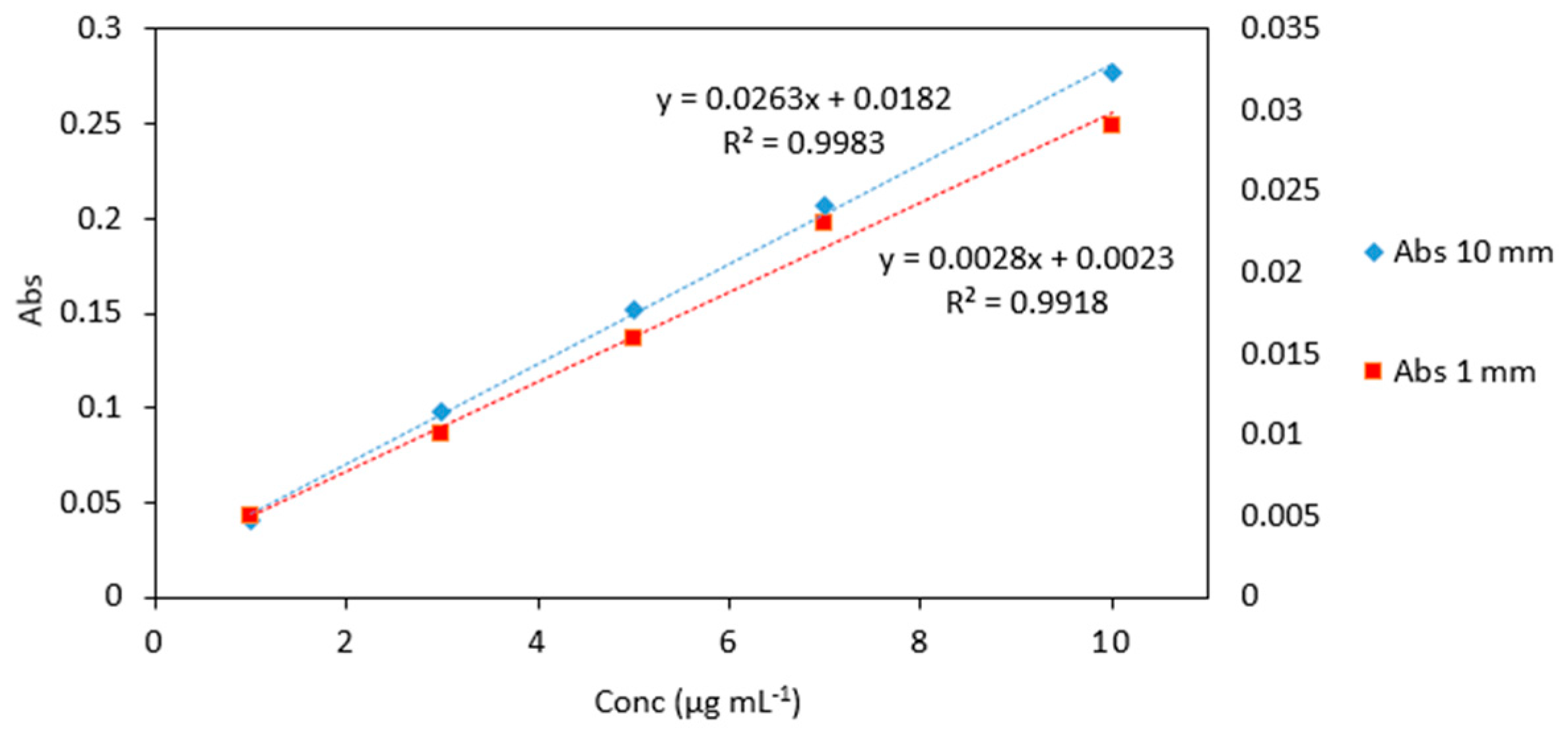
Figure 3.
Comparison of arsenic standards (1–10 µg mL−1) measured in quartz cuvettes with 10 mm and 1 mm path lengths. Left vertical axes represents the absorbance of standards analyzed in 10 mm quartz cuvettes (blue markers). Right vertical axes represents the absorbance of standards analyzed in 1 mm quartz microcuvettes (red markers). All measurements were carried out in triplicate.
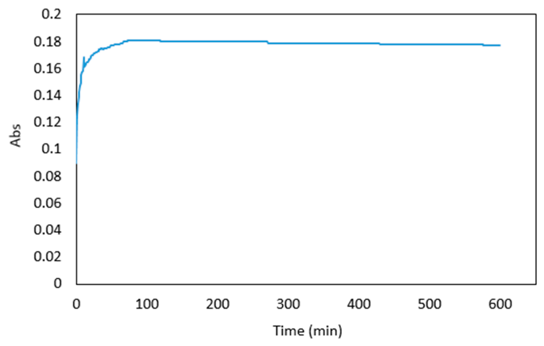
Figure 4.
Absorbance of 1 μg mL−1 arsenic sample premixed with the reagents over 600 min.
Figure 4.
Absorbance of 1 μg mL−1 arsenic sample premixed with the reagents over 600 min.
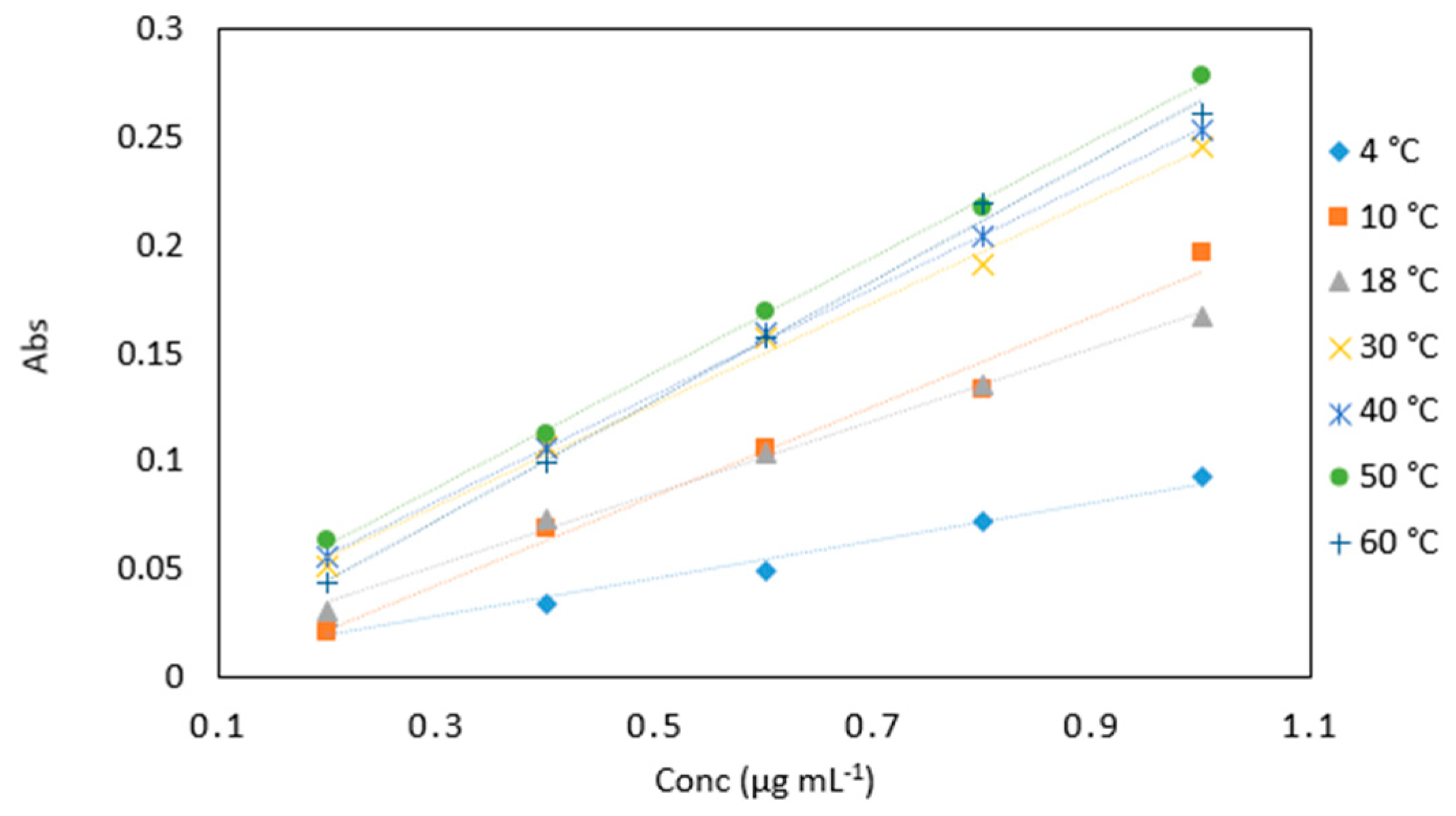
Figure 5.
A comparison of arsenic samples (0.2–1 µg mL−1) analyzed at various incubation temperatures (4, 10, 18, 30, 40, 50 and 60 °C). All measurements were carried out in triplicate (n = 105).
Figure 5.
A comparison of arsenic samples (0.2–1 µg mL−1) analyzed at various incubation temperatures (4, 10, 18, 30, 40, 50 and 60 °C). All measurements were carried out in triplicate (n = 105).
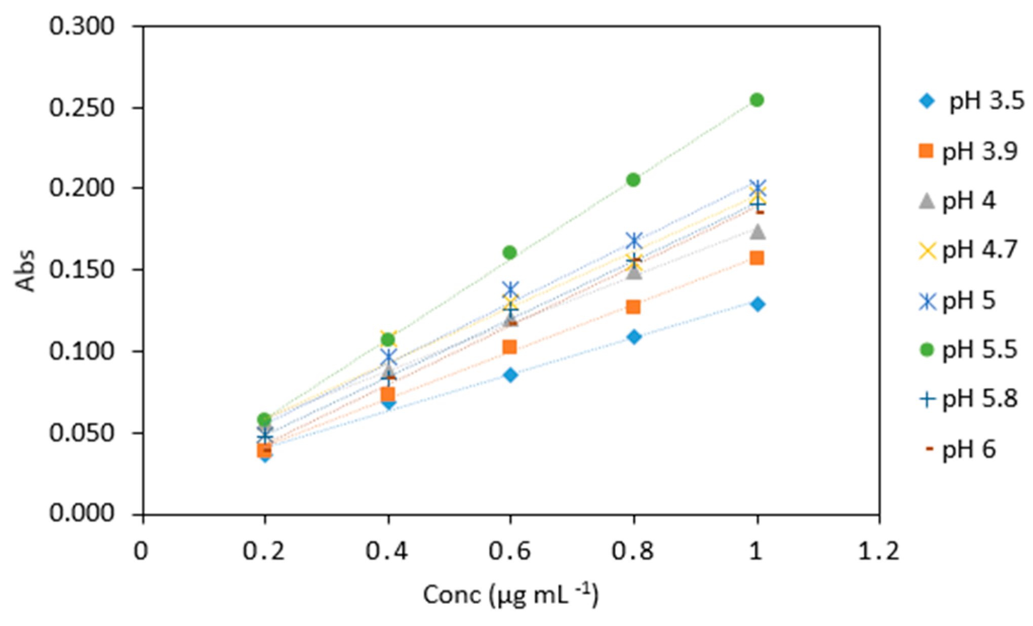
Figure 6.
Comparison of arsenic samples (0.2–1 µg mL−1) analyzed using various sodium triacetate buffers (pH 3.5, 3.9, 4, 4.7, 5, 5.5, 5.8, 6). All measurements were carried out in triplicate (n = 120).
Figure 6.
Comparison of arsenic samples (0.2–1 µg mL−1) analyzed using various sodium triacetate buffers (pH 3.5, 3.9, 4, 4.7, 5, 5.5, 5.8, 6). All measurements were carried out in triplicate (n = 120).
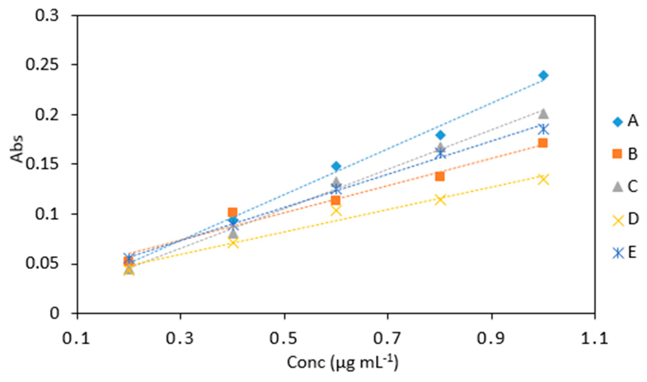
Figure 7.
A comparison of arsenic samples (0.2–1 µg mL−1) analyzed using several reagent ratios: (A), 6 (As): 1(KIO3): 0.5 (1 M HCl): 0.5: (LMG): 2 (sodium triacetate buffer), (B), 6 (As): 2.5 (KIO3): 2.5 (0.2 M HCl): 2.5: (LMG and buffer), (C), 6 (As): 2.5 (KIO3 and 0.4 M HCl): 2.5 (LMG and buffer), (D), 2 (As): 2 (1% KIO3 and 0.4 M HCl): 2 (LMG and sodium triacetate buffer) and (E) 2 (As): 1(1% KIO3 and 0.4 M HCl): 1 (LMG and sodium triacetate buffer).
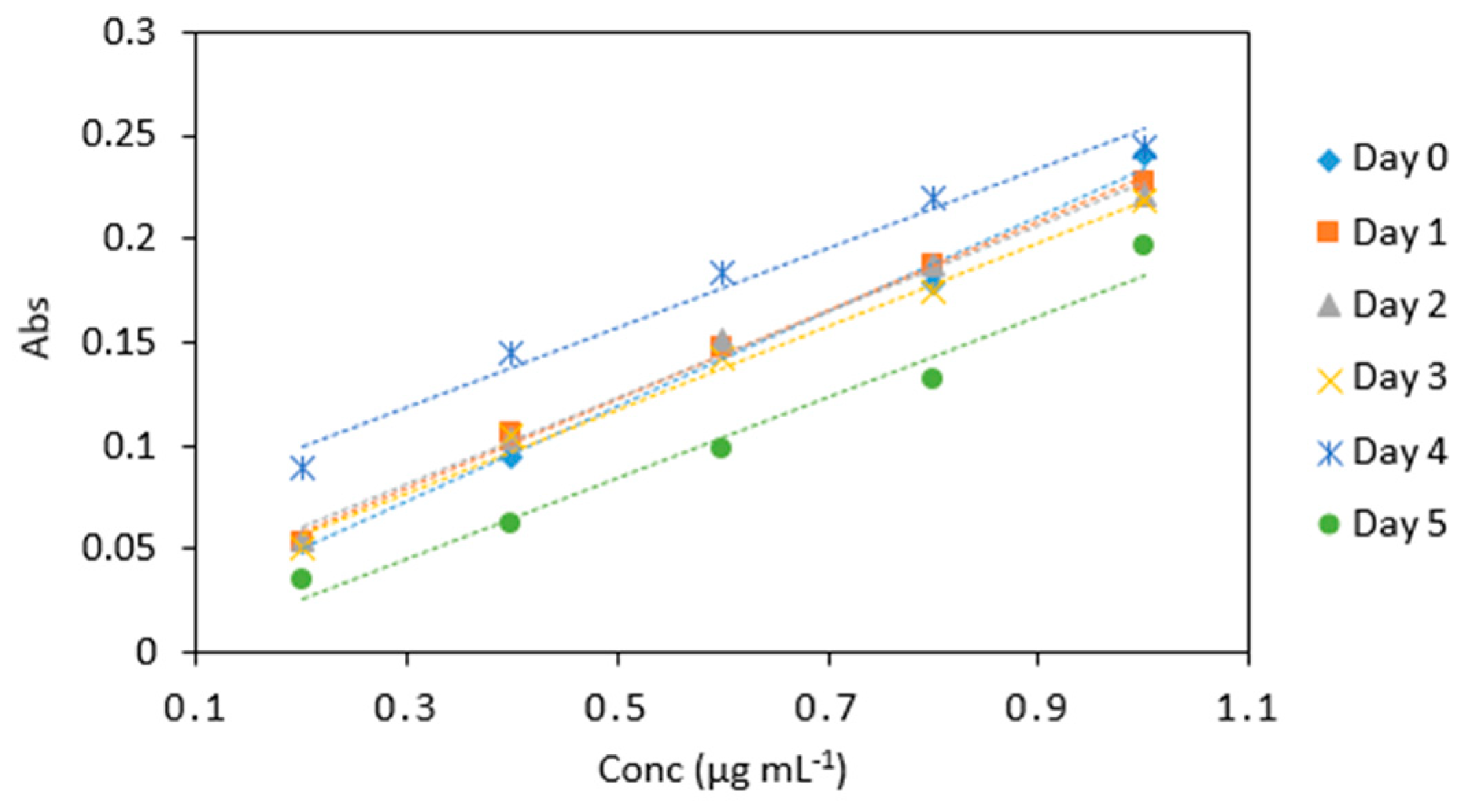
Figure 8.
Stability of potassium iodate and hydrochloric acid mix in arsenic samples (0.2–1 µg mL−1) analyzed periodically over day 0, 1, 2, 3, 4, and 5. All measurements were carried out in triplicate (n = 90).
Figure 8.
Stability of potassium iodate and hydrochloric acid mix in arsenic samples (0.2–1 µg mL−1) analyzed periodically over day 0, 1, 2, 3, 4, and 5. All measurements were carried out in triplicate (n = 90).
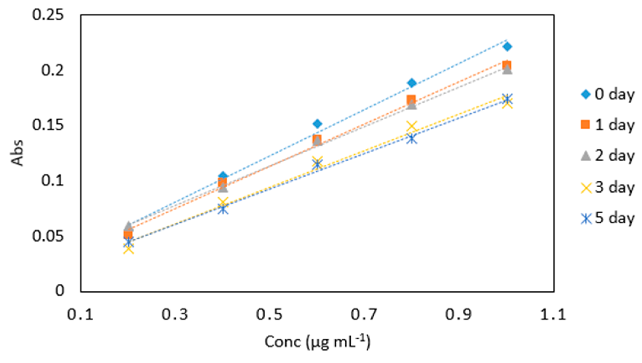
Figure 9.
Comparison of arsenic samples (0.2–1 µg mL−1) analyzed periodically on day 0, 1, 2, 3 and 5 under the same conditions with the leucomalachite green dye and in sodium triacetate buffer (pH 5.5). All measurements were carried out in triplicate (n = 75).
Figure 9.
Comparison of arsenic samples (0.2–1 µg mL−1) analyzed periodically on day 0, 1, 2, 3 and 5 under the same conditions with the leucomalachite green dye and in sodium triacetate buffer (pH 5.5). All measurements were carried out in triplicate (n = 75).
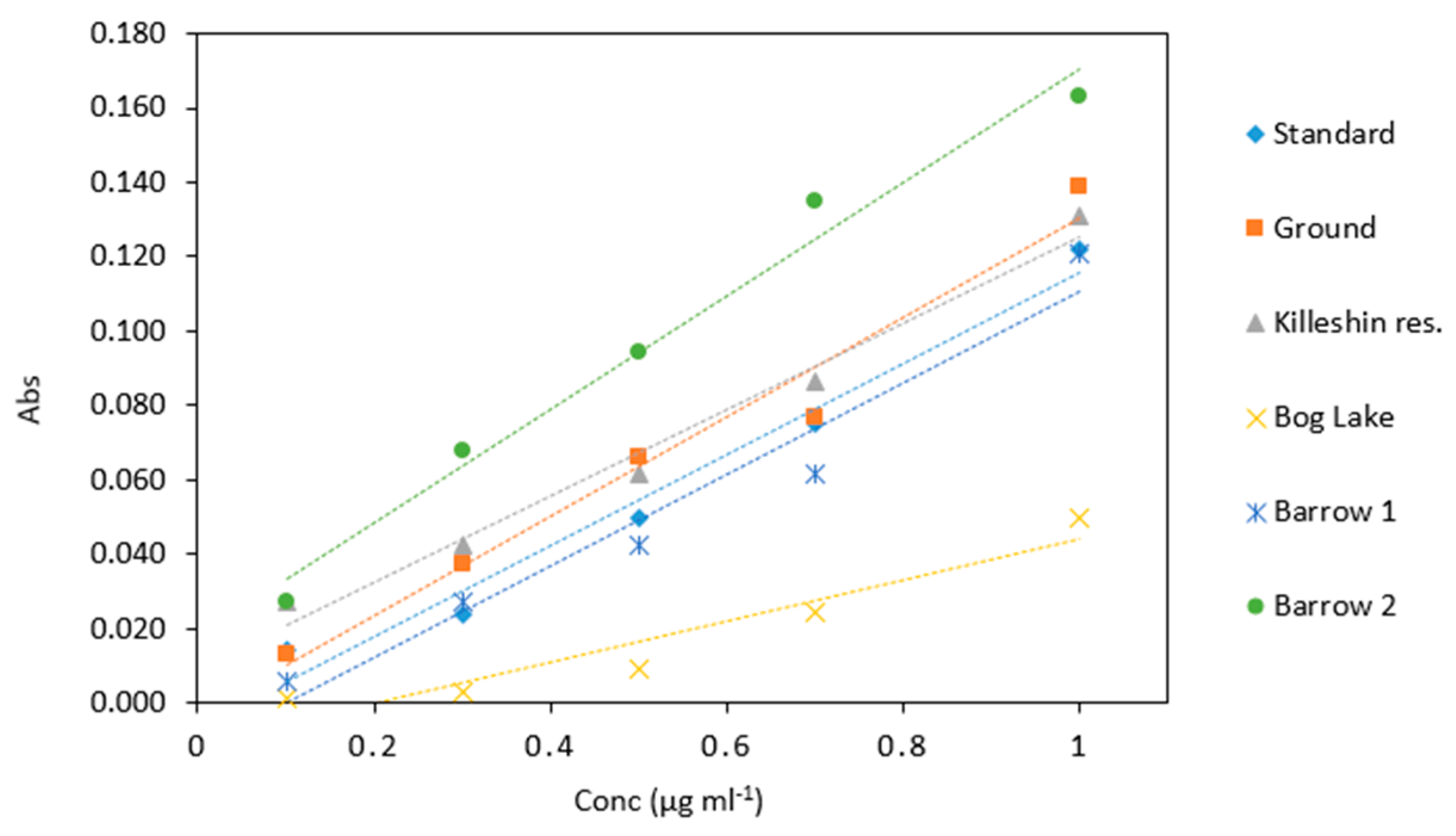
Figure 10.
Comparison of arsenic samples (0.1–1 µg mL−1) analyzed in several water matrices. All measurements were carried out in triplicate (n = 90).
Figure 10.
Comparison of arsenic samples (0.1–1 µg mL−1) analyzed in several water matrices. All measurements were carried out in triplicate (n = 90).
Table 1.
Average absorbance values for arsenic samples (0.2–1 µg mL−1) analyzed in two different types of cuvettes. Abs 1, SD 1 and % RSD 1 show the data for measurements carried out with 10 mm quartz cuvettes. Abs 2, SD 2 and % RSD 2 show the data for measurements in 1 mm quartz cuvettes. All measurements were carried out in triplicate (n = 30).
| Conc (µg mL−1) | Abs 1 | Abs 2 | SD 1 | SD 2 | % RSD 1 | % RSD 2 |
|---|
| 1 | 0.041 | 0.005 | 0.003 | 0.001 | 6.089 | 16.33 |
| 3 | 0.098 | 0.01 | 0.002 | 0 | 2.365 | 0 |
| 5 | 0.152 | 0.016 | 0.001 | 0 | 0.379 | 2.886 |
| 7 | 0.207 | 0.023 | 0.002 | 0.003 | 0.746 | 12.298 |
| 10 | 0.277 | 0.029 | 0.003 | 0 | 1.083 | 1.607 |
Table 2.
Effect of foreign species on the determination of arsenic (III) (1 µg mL−1).
Table 2.
Effect of foreign species on the determination of arsenic (III) (1 µg mL−1).
| Interferents | Tolerance Limit (μg mL−1) |
|---|
| Mn, Mg, PO4, NO3 | 100 |
| Fe (II) | 0.1 |
| EDTA | 3800 |
| Citric acid | 100,000 |
| Trimethylethanolamine | 450 |
Table 3.
Average absorbance values of arsenic samples (0.2–1 µg mL−1) analyzed at various incubation temperatures (4, 10, 18, 30, 40, 50 and 60 °C). All measurements were carried out in triplicate (n = 105).
Table 3.
Average absorbance values of arsenic samples (0.2–1 µg mL−1) analyzed at various incubation temperatures (4, 10, 18, 30, 40, 50 and 60 °C). All measurements were carried out in triplicate (n = 105).
| Temperature |
|---|
| Conc (µg mL−1) | 4 °C | 10 °C | 18 °C | 30 °C | 40 °C | 50 °C | 60 °C |
|---|
| 0.2 | 0.024 | 0.021 | 0.030 | 0.051 | 0.056 | 0.063 | 0.044 |
| 0.4 | 0.034 | 0.069 | 0.073 | 0.107 | 0.106 | 0.113 | 0.099 |
| 0.6 | 0.049 | 0.106 | 0.104 | 0.157 | 0.159 | 0.169 | 0.157 |
| 0.8 | 0.072 | 0.133 | 0.135 | 0.191 | 0.204 | 0.217 | 0.220 |
| 1 | 0.093 | 0.197 | 0.167 | 0.246 | 0.254 | 0.279 | 0.261 |
| Slope | 0.088 | 0.208 | 0.168 | 0.243 | 0.253 | 0.273 | 0.270 |
| R2 | 0.977 | 0.983 | 0.995 | 0.996 | 0.999 | 0.999 | 0.997 |
Table 4.
Average absorbance of arsenic samples (0.2–1 µg mL−1) analyzed with various sodium triacetate buffer pH. All measurements were carried out in triplicate (n = 120).
Table 4.
Average absorbance of arsenic samples (0.2–1 µg mL−1) analyzed with various sodium triacetate buffer pH. All measurements were carried out in triplicate (n = 120).
| Conc (µg mL−1) | pH 3.5 | pH 3.9 | pH 4 | pH 4.7 | pH 5 | pH 5.5 | pH 5.8 | pH 6 |
|---|
| 0.2 | 0.037 | 0.039 | 0.057 | 0.048 | 0.057 | 0.057 | 0.048 | 0.038 |
| 0.4 | 0.068 | 0.074 | 0.088 | 0.108 | 0.106 | 0.106 | 0.083 | 0.084 |
| 0.6 | 0.085 | 0.102 | 0.120 | 0.13 | 0.161 | 0.161 | 0.125 | 0.116 |
| 0.8 | 0.109 | 0.127 | 0.149 | 0.154 | 0.205 | 0.205 | 0.155 | 0.156 |
| 1 | 0.129 | 0.157 | 0.174 | 0.196 | 0.254 | 0.254 | 0.190 | 0.185 |
| Slope | 0.126 | 0.081 | 0.168 | 0.171 | 0.200 | 0.253 | 0.188 | 0.188 |
| R2 | 0.983 | 0.989 | 0.979 | 0.968 | 0.990 | 0.999 | 0.995 | 0.997 |
Table 5.
Average absorbance of arsenic samples (0.2–1 µg mL−1) analyzed using various reagent ratios: (A), 6 (As): 1(KIO3): 0.5 (1 M HCl): 0.5: (LMG): 2 (sodium triacetate buffer), (B), 6 (As): 2.5 (KIO3): 2.5 (0.2 M HCl): 2.5: (LMG and buffer), (C), 6 (As): 2.5 (KIO3 and 0.4 M HCl): 2.5 (LMG and buffer), (D), 2 (As): 2 (1% KIO3 and 0.4 M HCl): 2 (LMG and sodium triacetate buffer) and (E) 2 (As): 1(1% KIO3 and 0.4 M HCl): 1 (LMG and sodium triacetate buffer). All measurements were carried out in triplicate (n = 75).
| Reagent Ratio |
|---|
| Conc (µg mL−1) | A | B | C | D | E |
|---|
| 0.2 | 0.053 | 0.052 | 0.045 | 0.043 | 0.056 |
| 0.4 | 0.094 | 0.101 | 0.081 | 0.071 | 0.089 |
| 0.6 | 0.148 | 0.113 | 0.132 | 0.104 | 0.126 |
| 0.8 | 0.179 | 0.137 | 0.168 | 0.114 | 0.162 |
| 1 | 0.240 | 0.171 | 0.201 | 0.135 | 0.186 |
| Slope | 0.232 | 0.160 | 0.203 | 0.114 | 0.167 |
| R2 | 0.996 | 0.957 | 0.996 | 0.971 | 0.996 |
Table 6.
Average absorbance values for arsenic samples (0.2–1 µg mL−1) analyzed periodically on day 0, 1, 2, 3, 4 and 5 under the same conditions with the same potassium iodate and hydrochloric acid mix. All measurements were carried out in triplicate (n = 90).
Table 6.
Average absorbance values for arsenic samples (0.2–1 µg mL−1) analyzed periodically on day 0, 1, 2, 3, 4 and 5 under the same conditions with the same potassium iodate and hydrochloric acid mix. All measurements were carried out in triplicate (n = 90).
| Time (Days) |
|---|
| Conc (µg mL−1) | 0 | 1 | 2 | 3 | 4 | 5 |
|---|
| 0.2 | 0.089 | 0.053 | 0.055 | 0.053 | 0.051 | 0.036 |
| 0.4 | 0.145 | 0.106 | 0.104 | 0.094 | 0.105 | 0.062 |
| 0.6 | 0.184 | 0.147 | 0.151 | 0.148 | 0.142 | 0.098 |
| 0.8 | 0.220 | 0.187 | 0.188 | 0.179 | 0.175 | 0.132 |
| 1 | 0.244 | 0.228 | 0.221 | 0.240 | 0.218 | 0.196 |
| Slope | 0.193 | 0.216 | 0.208 | 0.233 | 0.202 | 0.186 |
| R2 | 0.978 | 0.997 | 0.993 | 0.995 | 0.993 | 0.978 |
Table 7.
Average absorbance for arsenic samples (0.2–1 µg mL−1) analyzed periodically on day 0, 1, 2, 3, 4 and 5 under the same conditions with the same dye and buffer mix. All measurements were carried out in triplicate (n = 75).
Table 7.
Average absorbance for arsenic samples (0.2–1 µg mL−1) analyzed periodically on day 0, 1, 2, 3, 4 and 5 under the same conditions with the same dye and buffer mix. All measurements were carried out in triplicate (n = 75).
| Time (Days) |
|---|
| Conc (µg mL−1) | 0 | 1 | 2 | 3 | 5 |
|---|
| 0.2 | 0.055 | 0.051 | 0.059 | 0.039 | 0.044 |
| 0.4 | 0.104 | 0.098 | 0.094 | 0.081 | 0.075 |
| 0.6 | 0.151 | 0.137 | 0.136 | 0.118 | 0.115 |
| 0.8 | 0.188 | 0.173 | 0.168 | 0.149 | 0.138 |
| 1 | 0.221 | 0.204 | 0.201 | 0.170 | 0.174 |
| Slope | 0.223 | 0.191 | 0.178 | 0.166 | 0.161 |
| R2 | 0.996 | 0.994 | 0.977 | 0.986 | 0.996 |
Table 8.
The average absorbance of arsenic samples (0.1–1 µg mL−1) analyzed in different water matrices. The measurements were carried out in triplicate (n = 90).
Table 8.
The average absorbance of arsenic samples (0.1–1 µg mL−1) analyzed in different water matrices. The measurements were carried out in triplicate (n = 90).
| Water Samples |
|---|
| Conc (µg mL−1) | Control | Ground | Killeshin Res. | Bog Lake | Barrow 1 | Barrow 2 |
|---|
| 0.1 | 0.014 | 0.013 | 0.027 | 0.001 | 0.006 | 0.027 |
| 0.3 | 0.024 | 0.037 | 0.042 | 0.003 | 0.027 | 0.068 |
| 0.5 | 0.050 | 0.066 | 0.061 | 0.009 | 0.042 | 0.094 |
| 0.7 | 0.075 | 0.077 | 0.087 | 0.024 | 0.061 | 0.135 |
| 1 | 0.122 | 0.139 | 0.131 | 0.050 | 0.121 | 0.163 |
| Slope | 0.114 | 0.135 | 0.104 | 0.072 | 0.123 | 0.090 |
| R2 | 0.996 | 0.978 | 0.996 | 0.996 | 0.955 | 0.999 |


