Chemically Responsive Hydrogel Deformation Mechanics: A Review


Abstract
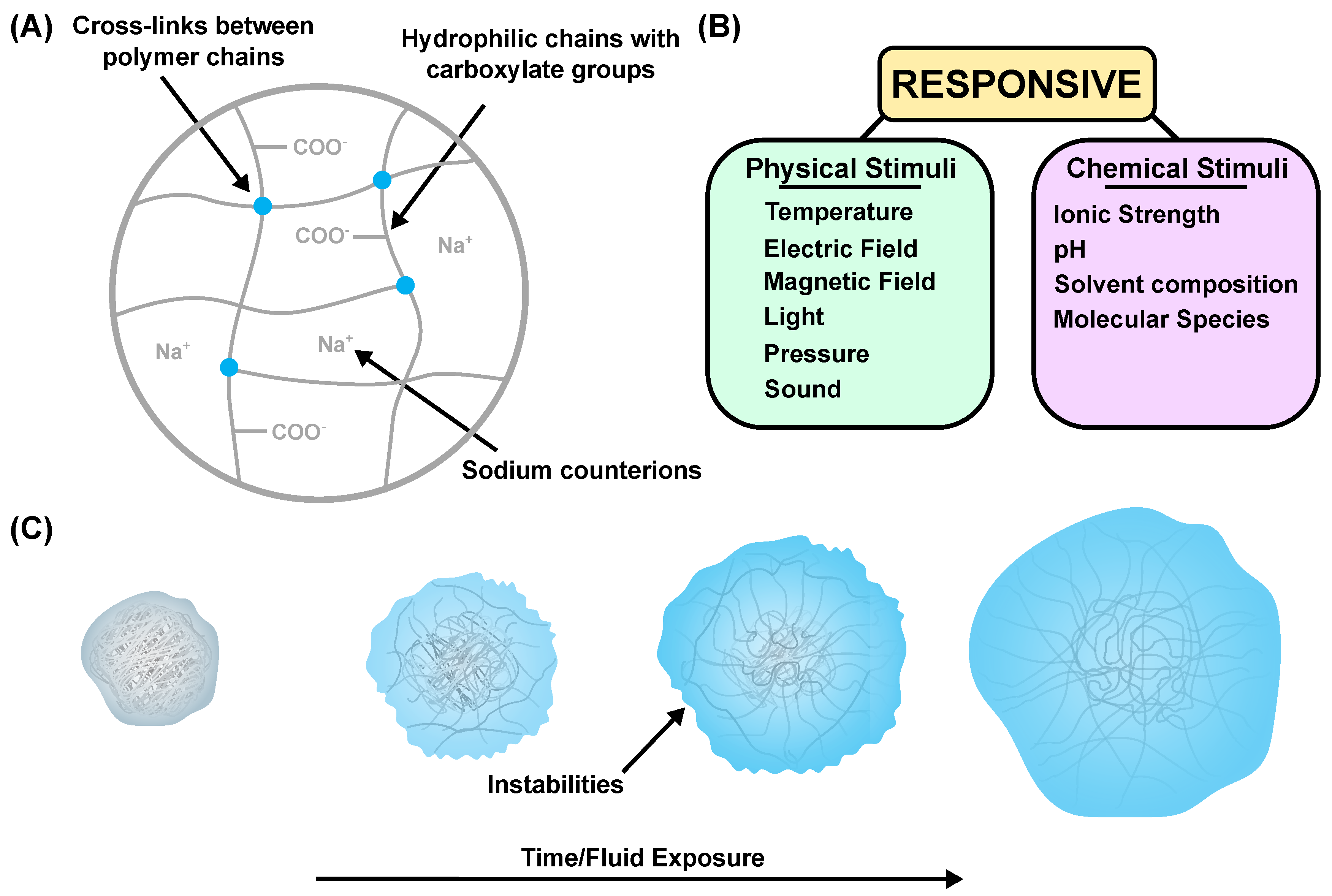
1. Introduction
2. Hydrogel Swelling Theory
2.1. Mixing Energy
2.2. Ionic Energy
2.3. Elastic Energy
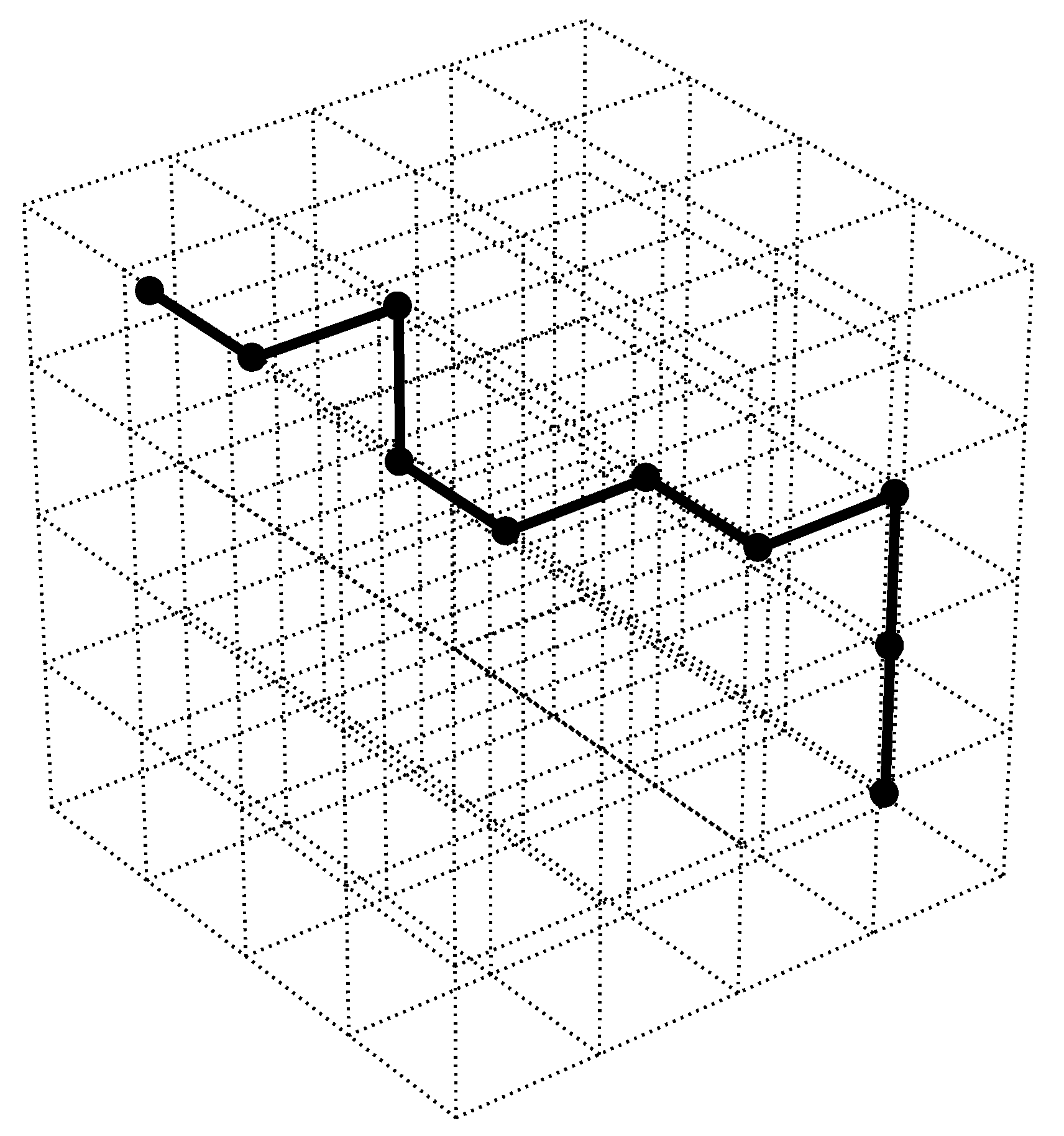
2.3.1. Statistical Mechanics: Flory–Rehner Theory
2.3.2. Continuum Mechanics: Mixture Theory
3. Experimental Analysis
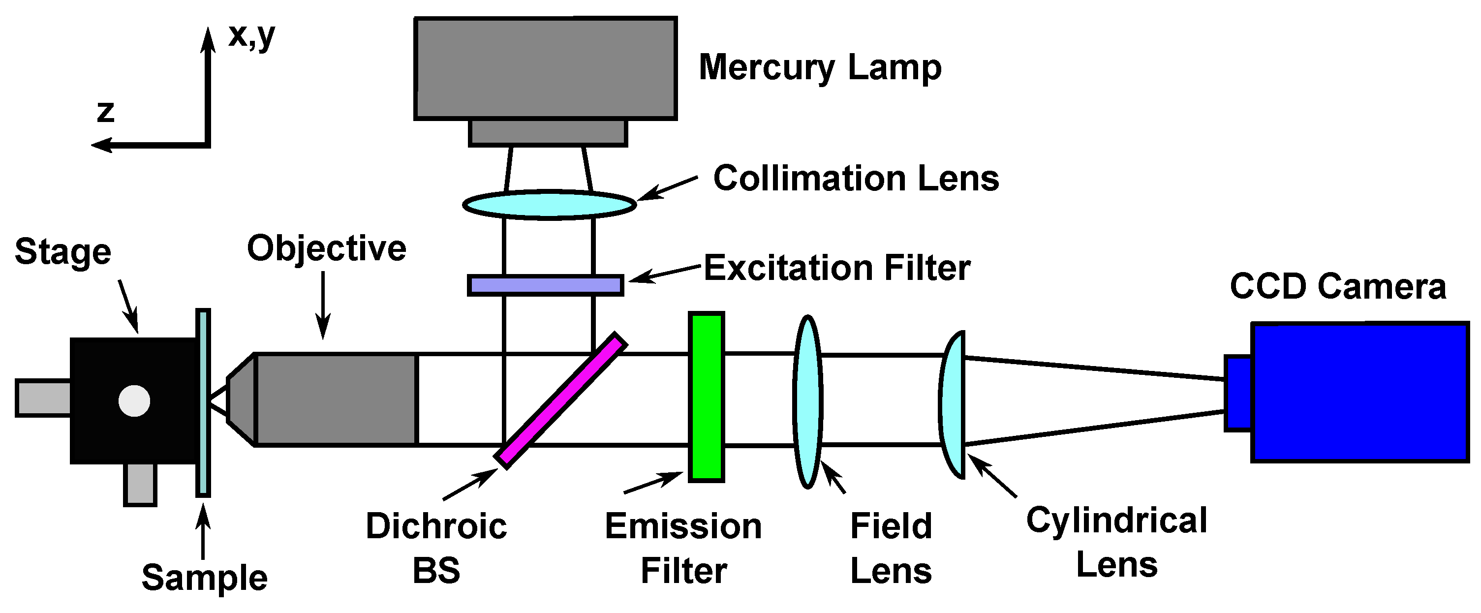
3.1. Deformation Measurements
3.2. Mechanical Behavior
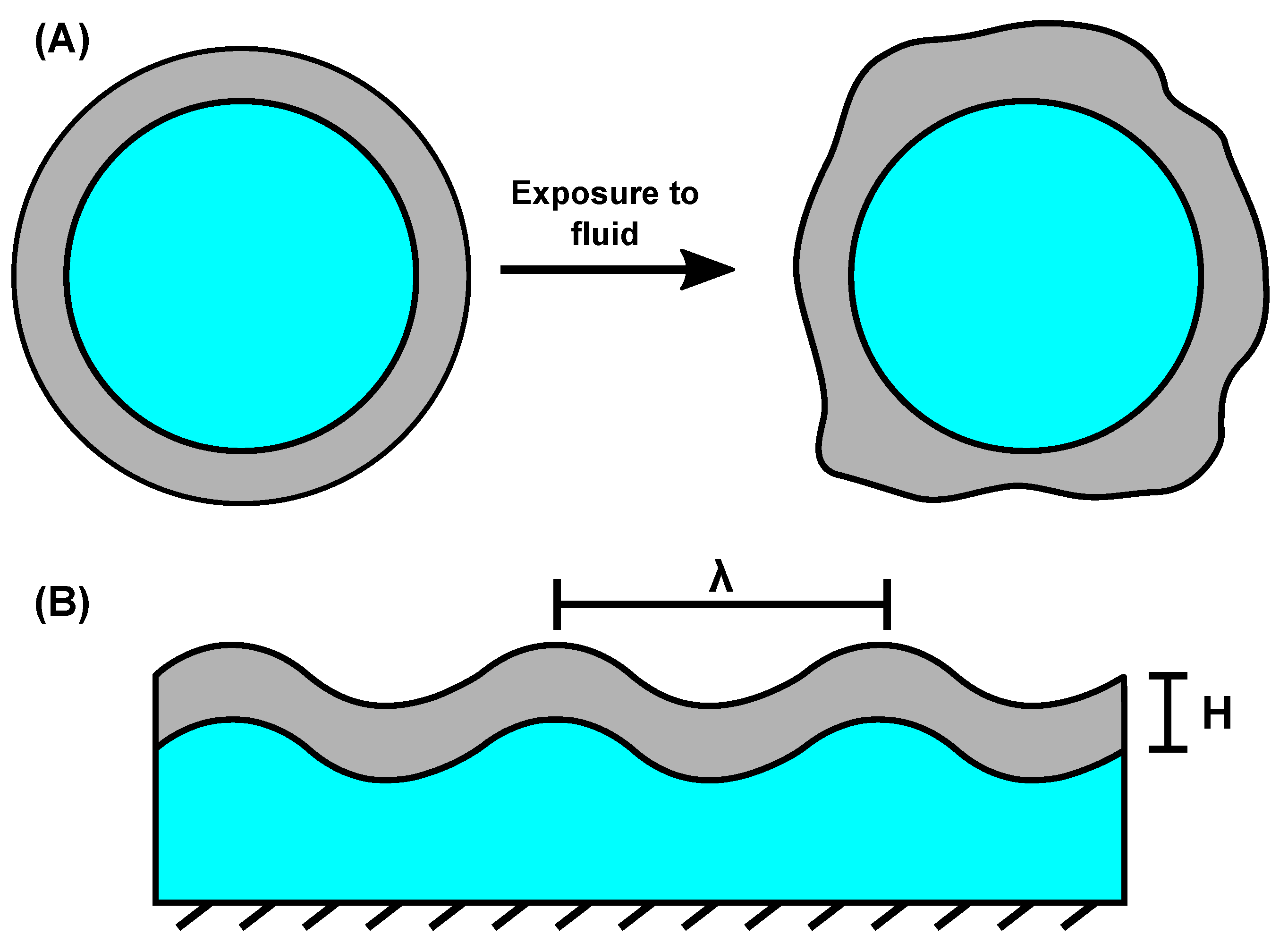
4. Transient Surface Instabilities
5. Conclusions
Author Contributions
Funding
Acknowledgments
Conflicts of Interest
Abbreviations
| 2D | Two-Dimensional |
| 3D | Three-Dimensional |
| CCD | Charged Couple Device |
| CMOS | Complementary Metal Oxide Semiconductor |
| CRC | Centrifuge Retention Capacity |
| DIC | Digital Image Correlation |
| FEM | Finite Element Method |
| MHFEM | Mixed Hybrid Finite Element Method |
| MRI | Magnetic Resonance Imaging |
| NMR | Nuclear Magnetic Resonance |
| PTV | Particle Tracking Velocimetry |
| SAP | Superabsorbent Polymer |
| − (subscript) | Negative Charge |
| + (subscript) | Positive Charge |
| Avagadro’s Number | |
| Boltzmann Constant | |
| C | Capacity |
| Change in energy for the formation of a polymer–solvent interaction | |
| Chemical Potential | |
| n and c | Concentration (amount-of-substance and molar) |
| (subscript) | Constituent |
| CI | Counter-ion |
| Deformation of the system (Statistical Mechanics) | |
| F | Deformation Tensor |
| Density | |
| ∇ | Divergence operator |
| S | Entropy |
| T | First Piola–Kirchhoff stress tensor |
| Flory–Huggins Parameter | |
| Q | Fluid Flux |
| fluid specific mass | |
| G | Gibbs Free Energy |
| F | Helmholtz Free Energy |
| I | Identity Tensor |
| U | Internal Energy associated with Enthalpy |
| J | Determinant of the deformation tensor (Volume change) |
| Q | Lagrangian vector |
| Principal stretch | |
| Mixture theory mapping function | |
| M | Mass |
| G | Moduli |
| Molar chemical potential | |
| Molar Volume | |
| Number of elastic junctions | |
| z | Number of lattice connections |
| N | Number of molecules |
| Osmotic pressure | |
| k | Permeability |
| p (subscript) | polymer |
| p | pore pressure |
| r | Radius |
| r | repeat units |
| C | right Cauchy–Green strain tensor |
| S | second Piola–Kirchhoff stress tensor |
| s (subscript) | solvent |
| Stress | |
| T | Temperature |
| R | Universal Gas Constant |
| V | Volume |
| Volume Fraction |
References
- Ullah, F.; Othman, M.B.H.; Javed, F.; Ahmad, Z.; Akil, H.M. Classification, processing and application of hydrogels: A review. Mater. Sci. Eng. C 2015, 57, 414–433. [Google Scholar] [CrossRef] [PubMed]
- Boraston, A.B.; Bolam, D.N.; Gilbert, H.J.; Davies, G.J. Carbohydrate-binding modules: Fine-tuning polysaccharide recognition. Biochem. J. 2004, 382, 769–781. [Google Scholar] [CrossRef] [PubMed]
- Wichterle, O.; Lim, D. Hydrophilic gels for biological use. Nature 1960, 185, 117. [Google Scholar] [CrossRef]
- Ahmed, E.M. Hydrogel: Preparation, characterization, and applications: A review. J. Adv. Res. 2015, 6, 105–121. [Google Scholar] [CrossRef] [PubMed]
- Rubinstein, M.; Colby, R.H. Polymer Physics; Oxford University Press: New York, NY, USA, 2003; Volume 23. [Google Scholar]
- Ferry, J.D.; Ferry, J.D. Viscoelastic Properties of Polymers; John Wiley & Sons: Hoboken, NJ, USA, 1980. [Google Scholar]
- Buchholz, F.L.; Graham, A.T. Modern Superabsorbent Polymer Technology; John Wiley & Sons, Inc.: New York, NY, USA, 1998; p. 279. [Google Scholar]
- Zohuriaan-Mehr, M.J.; Kabiri, K. Superabsorbent polymer materials: A review. Iran. Polym. J. 2008, 17, 451. [Google Scholar]
- Qiu, Y.; Park, K. Environment-sensitive hydrogels for drug delivery. Adv. Drug Deliv. Rev. 2001, 53, 321–339. [Google Scholar] [CrossRef]
- Bertrand, T.; Peixinho, J.; Mukhopadhyay, S.; MacMinn, C.W. Dynamics of swelling and drying in a spherical gel. Phys. Rev. Appl. 2016, 6, 064010. [Google Scholar] [CrossRef]
- Yu, C.; Malakpoor, K.; Huyghe, J.M. A three-dimensional transient mixed hybrid finite element model for superabsorbent polymers with strain-dependent permeability. Soft Matter 2018, 14, 3834–3848. [Google Scholar] [CrossRef]
- Rimmer, S. Biomedical Hydrogels: Biochemistry, Manufacture and Medical Applications; Elsevier: Amsterdam, The Netherlands, 2011. [Google Scholar]
- Hoffman, A.S. Hydrogels for biomedical applications. Adv. Drug Deliv. Rev. 2012, 64, 18–23. [Google Scholar] [CrossRef]
- Sannino, A.; Demitri, C.; Madaghiele, M. Biodegradable cellulose-based hydrogels: Design and applications. Materials 2009, 2, 353–373. [Google Scholar] [CrossRef]
- Narjary, B.; Aggarwal, P.; Singh, A.; Chakraborty, D.; Singh, R. Water availability in different soils in relation to hydrogel application. Geoderma 2012, 187, 94–101. [Google Scholar] [CrossRef]
- Caló, E.; Khutoryanskiy, V.V. Biomedical applications of hydrogels: A review of patents and commercial products. Eur. Polym. J. 2015, 65, 252–267. [Google Scholar] [CrossRef]
- Hong, W.; Zhao, X.; Zhou, J.; Suo, Z. A theory of coupled diffusion and large deformation in polymeric gels. J. Mech. Phys. Solids 2008, 56, 1779–1793. [Google Scholar] [CrossRef]
- Flory, P.J.; Tatara, Y.I. The elastic free energy and the elastic equation of state: Elongation and swelling of polydimethylsiloxane networks. J. Polym. Sci. Polym. Phys. Ed. 1975, 13, 683–702. [Google Scholar] [CrossRef]
- McKenna, G.B.; Flynn, K.M.; Chen, Y. Experiments on the elasticity of dry and swollen networks: Implications for the Frenkel-Flory-Rehner hypothesis. Macromolecules 1989, 22, 4507–4512. [Google Scholar] [CrossRef]
- Gumbrell, S.; Mullins, L.; Rivlin, R. Departures of the elastic behaviour of rubbers in simple extension from the kinetic theory. Trans. Faraday Soc. 1953, 49, 1495–1505. [Google Scholar] [CrossRef]
- Quesada-Pérez, M.; Maroto-Centeno, J.A.; Forcada, J.; Hidalgo-Alvarez, R. Gel swelling theories: The classical formalism and recent approaches. Soft Matter 2011, 7, 10536–10547. [Google Scholar] [CrossRef]
- Li, J.; Hu, Y.; Vlassak, J.J.; Suo, Z. Experimental determination of equations of state for ideal elastomeric gels. Soft Matter 2012, 8, 8121–8128. [Google Scholar] [CrossRef]
- Capriles-González, D.; Sierra-Martín, B.; Fernández-Nieves, A.; Fernández-Barbero, A. Coupled deswelling of multiresponse microgels. J. Phys. Chem. B 2008, 112, 12195–12200. [Google Scholar] [CrossRef]
- Mann, B.A.; Holm, C.; Kremer, K. Swelling of polyelectrolyte networks. J. Chem. Phys. 2005, 122, 154903. [Google Scholar] [CrossRef]
- Roos, R.W.; Petterson, R.; Huyghe, J.M. Confined compression and torsion experiments on a pHEMA gel in various bath concentrations. Biomech. Model. Mechanobiol. 2013, 12, 617–626. [Google Scholar] [CrossRef] [PubMed][Green Version]
- Khokhlov, A.R.; Starodubtzev, S.G.; Vasilevskaya, V.V. Conformational transitions in polymer gels: Theory and experiment. In Responsive Gels: Volume Transitions I; Springer: Berlin/Heidelberg, Germany, 1993; pp. 123–171. [Google Scholar]
- De Boer, R. Theory of Porous Media: Highlights in Historical Development and Current State; Springer Science & Business Media: Berlin/Heidelberg, Germany, 2012. [Google Scholar]
- Flory, P.J. Thermodynamics of high polymer solutions. J. Chem. Phys. 1941, 9, 660. [Google Scholar] [CrossRef]
- Huggins, M.L. Some properties of solutions of long-chain compounds. J. Phys. Chem. 1942, 46, 151–158. [Google Scholar] [CrossRef]
- Flory, P.J. Principles of Polymer Chemistry; Cornell University Press: Ithaca, NY, USA, 1953. [Google Scholar]
- Orofino, T.A.; Flory, P. Relationship of the second virial coefficient to polymer chain dimensions and interaction parameters. J. Chem. Phys. 1957, 26, 1067–1076. [Google Scholar] [CrossRef]
- Erman, B.; Flory, P. Critical phenomena and transitions in swollen polymer networks and in linear macromolecules. Macromolecules 1986, 19, 2342–2353. [Google Scholar] [CrossRef]
- Hill, T.L. An Introduction to Statistical Thermodynamics; Courier Corporation: North Chelmsford, MA, USA, 1986. [Google Scholar]
- Li, H.; Wang, X.; Yan, G.; Lam, K.; Cheng, S.; Zou, T.; Zhuo, R. A novel multiphysic model for simulation of swelling equilibrium of ionized thermal-stimulus responsive hydrogels. Chem. Phys. 2005, 309, 201–208. [Google Scholar] [CrossRef]
- Li, H.; Lai, F. Multiphysics modeling of responsive characteristics of ionic-strength-sensitive hydrogel. Biomed. Microdevices 2010, 12, 419–434. [Google Scholar] [CrossRef]
- Longo, G.S.; Olvera de La Cruz, M.; Szleifer, I. Molecular theory of weak polyelectrolyte gels: The role of pH and salt concentration. Macromolecules 2010, 44, 147–158. [Google Scholar] [CrossRef]
- Wallmersperger, T.; Keller, K.; Kröplin, B.; Günther, M.; Gerlach, G. Modeling and simulation of pH-sensitive hydrogels. Colloid Polym. Sci. 2011, 289, 535. [Google Scholar] [CrossRef]
- Flory, P.J.; Rehner, J., Jr. Statistical mechanics of cross-linked polymer networks I. Rubberlike elasticity. J. Chem. Phys. 1943, 11, 512–520. [Google Scholar] [CrossRef]
- Horkay, F.; McKenna, G.B. Polymer networks and gels. In Physical Properties of Polymers Handbook; Springer: Berlin/Heidelberg, Germany, 2007; pp. 497–523. [Google Scholar]
- James, H.M.; Guth, E. Theory of the increase in rigidity of rubber during cure. J. Chem. Phys. 1947, 15, 669–683. [Google Scholar] [CrossRef]
- Flory, P.J.; Erman, B. Theory of elasticity of polymer networks. 3. Macromolecules 1982, 15, 800–806. [Google Scholar] [CrossRef]
- Kloczkowski, A.; Mark, J.E.; Erman, B. A diffused-constraint theory for the elasticity of amorphous polymer networks. 1. Fundamentals and stress-strain isotherms in elongation. Macromolecules 1995, 28, 5089–5096. [Google Scholar] [CrossRef]
- Doi, M. Explanation for the 3.4-power law for viscosity of polymeric liquids on the basis of the tube model. J. Polym. Sci. Polym. Phys. Ed. 1983, 21, 667–684. [Google Scholar] [CrossRef]
- Wall, F.T. Statistical thermodynamics of rubber. III. J. Chem. Phys. 1943, 11, 527–530. [Google Scholar] [CrossRef]
- Yen, L.; Eichinger, B. Volume dependence of the elastic equation of state. J. Polym. Sci. Polym. Phys. Ed. 1978, 16, 121–130. [Google Scholar] [CrossRef]
- Hermans, J. Deformation and swelling of polymer networks containing comparatively long chains. Trans. Faraday Soc. 1947, 43, 591–600. [Google Scholar] [CrossRef]
- Tanaka, T.; Fillmore, D.J. Kinetics of swelling of gels. J. Chem. Phys. 1979, 70, 1214–1218. [Google Scholar] [CrossRef]
- Zhang, J.; Zhao, X.; Suo, Z.; Jiang, H. A finite element method for transient analysis of concurrent large deformation and mass transport in gels. J. Appl. Phys. 2009, 105, 093522. [Google Scholar] [CrossRef]
- Chester, S.A.; Anand, L. A coupled theory of fluid permeation and large deformations for elastomeric materials. J. Mech. Phys. Solids 2010, 58, 1879–1906. [Google Scholar] [CrossRef]
- Duda, F.P.; Souza, A.C.; Fried, E. A theory for species migration in a finitely strained solid with application to polymer network swelling. J. Mech. Phys. Solids 2010, 58, 515–529. [Google Scholar] [CrossRef]
- MacMinn, C.W.; Dufresne, E.R.; Wettlaufer, J.S. Large deformations of a soft porous material. Phys. Rev. Appl. 2016, 5, 044020. [Google Scholar] [CrossRef]
- Biot, M.A. General theory of three-dimensional consolidation. J. Appl. Phys. 1941, 12, 155–164. [Google Scholar] [CrossRef]
- Coussy, O. Poromechanics; John Wiley & Sons: New York, NY, USA, 2004. [Google Scholar]
- Terzaghi, K.V. The shearing resistance of saturated soils and the angle between the planes of shear. In Proceedings of the First International Conference on Soil Mechanics, Cambridge, MA, USA, 22–26 June 1936; Volume 1, pp. 54–59. [Google Scholar]
- Biot, M.A.; Temple, G. Theory of finite deformations of porous solids. Indiana Univ. Math. J. 1972, 21, 597–620. [Google Scholar] [CrossRef]
- Rivlin, R. Large elastic deformations of isotropic materials IV. Further developments of the general theory. Philos. Trans. R. Soc. London. Ser. A Math. Phys. Sci. 1948, 241, 379–397. [Google Scholar] [CrossRef]
- Treloar, L.R.G. The Physics of Rubber Elasticity; Oxford University Press: Oxford, MI, USA, 1975. [Google Scholar]
- Mooney, M. A theory of large elastic deformation. J. Appl. Phys. 1940, 11, 582–592. [Google Scholar] [CrossRef]
- Basaran, S. Lagrangian and Eulerian Descriptions in Solid Mechanics and Their Numerical Solutions in hpk Framework. Ph.D. Thesis, University of Kansas, Lawrence, KS, USA, 2008. [Google Scholar]
- Hubbert, M.K. The theory of ground-water motion. J. Geol. 1940, 48, 785–944. [Google Scholar] [CrossRef]
- Truesdell, C.; Toupin, R. The classical field theories. In Principles of Classical Mechanics and Field Theory/Prinzipien der Klassischen Mechanik und Feldtheorie; Springer: Berlin/Heidelberg, Germany, 1960; pp. 226–858. [Google Scholar]
- Bowen, R.M. Incompressible porous media models by use of the theory of mixtures. Int. J. Eng. Sci. 1980, 18, 1129–1148. [Google Scholar] [CrossRef]
- Mow, V.C.; Kuei, S.; Lai, W.M.; Armstrong, C.G. Biphasic creep and stress relaxation of articular cartilage in compression: Theory and experiments. J. Biomech. Eng. 1980, 102, 73–84. [Google Scholar] [CrossRef]
- Lemon, G.; King, J.R.; Byrne, H.M.; Jensen, O.E.; Shakesheff, K.M. Mathematical modelling of engineered tissue growth using a multiphase porous flow mixture theory. J. Math. Biol. 2006, 52, 571–594. [Google Scholar] [CrossRef]
- Cowin, S.C.; Cardoso, L. Mixture theory-based poroelasticity as a model of interstitial tissue growth. Mech. Mater. 2012, 44, 47–57. [Google Scholar] [CrossRef] [PubMed]
- Lanir, Y. Biorheology and fluid flux in swelling tissues. I. Bicomponent theory for small deformations, including concentration effects. Biorheology 1987, 24, 173–187. [Google Scholar] [CrossRef] [PubMed]
- Lai, W.M.; Hou, J.; Mow, V.C. A triphasic theory for the swelling and deformation behaviors of articular cartilage. J. Biomech. Eng. 1991, 113, 245–258. [Google Scholar] [CrossRef] [PubMed]
- Huyghe, J.M.; Janssen, J. Quadriphasic mechanics of swelling incompressible porous media. Int. J. Eng. Sci. 1997, 35, 793–802. [Google Scholar] [CrossRef]
- Frijns, A.J.H.; Huyghe, J.; Janssen, J.D. A validation of the quadriphasic mixture theory for intervertebral disc tissue. Int. J. Eng. Sci. 1997, 35, 1419–1429. [Google Scholar] [CrossRef]
- Hong, W.; Liu, Z.; Suo, Z. Inhomogeneous swelling of a gel in equilibrium with a solvent and mechanical load. Int. J. Solids Struct. 2009, 46, 3282–3289. [Google Scholar] [CrossRef]
- Kang, M.K.; Huang, R. A variational approach and finite element implementation for swelling of polymeric hydrogels under geometric constraints. J. Appl. Mech. 2010, 77, 061004. [Google Scholar] [CrossRef]
- Van Loon, R.; Huyghe, J.; Wijlaars, M.; Baaijens, F. 3D FE implementation of an incompressible quadriphasic mixture model. Int. J. Numer. Methods Eng. 2003, 57, 1243–1258. [Google Scholar] [CrossRef]
- Bouklas, N.; Landis, C.M.; Huang, R. A nonlinear, transient finite element method for coupled solvent diffusion and large deformation of hydrogels. J. Mech. Phys. Solids 2015, 79, 21–43. [Google Scholar] [CrossRef]
- Brezzi, F.; Fortin, M. Mixed and Hybrid Finite Element Methods; Springer Science & Business Media: Berlin/Heidelberg, Germany, 2012; Volume 15. [Google Scholar]
- Levenston, M.; Frank, E.; Grodzinsky, A. Variationally derived 3-field finite element formulations for quasistatic poroelastic analysis of hydrated biological tissues. Comput. Methods Appl. Mech. Eng. 1998, 156, 231–246. [Google Scholar] [CrossRef]
- Vuong, A.T.; Yoshihara, L.; Wall, W. A general approach for modeling interacting flow through porous media under finite deformations. Comput. Methods Appl. Mech. Eng. 2015, 283, 1240–1259. [Google Scholar] [CrossRef]
- Kaasschieter, E.; Huijben, A. Mixed-hybrid finite elements and streamline computation for the potential flow problem. Numer. Methods Partial Differ. Equ. 1992, 8, 221–266. [Google Scholar] [CrossRef]
- Mosé, R.; Siegel, P.; Ackerer, P.; Chavent, G. Application of the mixed hybrid finite element approximation in a groundwater flow model: Luxury or necessity? Water Resour. Res. 1994, 30, 3001–3012. [Google Scholar] [CrossRef]
- Jha, B.; Juanes, R. A locally conservative finite element framework for the simulation of coupled flow and reservoir geomechanics. Acta Geotech. 2007, 2, 139–153. [Google Scholar] [CrossRef]
- Ferronato, M.; Castelletto, N.; Gambolati, G. A fully coupled 3-D mixed finite element model of Biot consolidation. J. Comput. Phys. 2010, 229, 4813–4830. [Google Scholar] [CrossRef]
- Malakpoor, K.; Kaasschieter, E.F.; Huyghe, J.M. Mathematical modelling and numerical solution of swelling of cartilaginous tissues. Part II: Mixed-hybrid finite element solution. ESAIM Math. Model. Numer. Anal. 2007, 41, 679–712. [Google Scholar] [CrossRef][Green Version]
- Lee, H.; Zhang, J.; Jiang, H.; Fang, N.X. Prescribed pattern transformation in swelling gel tubes by elastic instability. Phys. Rev. Lett. 2012, 108, 214304. [Google Scholar] [CrossRef]
- Oh, K.S.; Oh, J.S.; Choi, H.S.; Bae, Y.C. Effect of cross-linking density on swelling behavior of NIPA gel particles. Macromolecules 1998, 31, 7328–7335. [Google Scholar] [CrossRef]
- Dolbow, J.; Fried, E.; Ji, H. A numerical strategy for investigating the kinetic response of stimulus-responsive hydrogels. Comput. Methods Appl. Mech. Eng. 2005, 194, 4447–4480. [Google Scholar] [CrossRef]
- Bouklas, N.; Huang, R. Swelling kinetics of polymer gels: Comparison of linear and nonlinear theories. Soft Matter 2012, 8, 8194–8203. [Google Scholar] [CrossRef]
- Grosshans, D.; Knaebel, A.; Lequeux, F. Plasticity of an amorphous assembly of elastic gel beads. J. Phys. II 1995, 5, 53–62. [Google Scholar] [CrossRef]
- Knaebel, A.; Rebre, S.; Lequeux, F. Determination of the elastic modulus of superabsorbent gel beads. Polym. Gels Netw. 1997, 5, 107–121. [Google Scholar] [CrossRef]
- Tian, G.; Bergman, D.L., Jr.; Shi, Y. Superabsorbent Polymer Having a Capacity Increase. U.S. Patent 8,647,317, 6 November 2014. [Google Scholar]
- Schinagl, R.M.; Gurskis, D.; Chen, A.C.; Sah, R.L. Depth-dependent confined compression modulus of full-thickness bovine articular cartilage. J. Orthop. Res. 1997, 15, 499–506. [Google Scholar] [CrossRef] [PubMed]
- Briscoe, B.; Fiori, L.; Pelillo, E. Nano-indentation of polymeric surfaces. J. Phys. D Appl. Phys. 1998, 31, 2395. [Google Scholar] [CrossRef]
- Oyen, M.L. Nanoindentation of hydrated materials and tissues. Curr. Opin. Solid State Mater. Sci. 2015, 19, 317–323. [Google Scholar] [CrossRef]
- Lindner, T.; Morand, M.; Meyer, A.; Tremel, M.; Weaver, M.R. Method for Determining the Gel Strength of a Hydrogel. U.S. Patent 8,653,321, 18 February 2014. [Google Scholar]
- Karadimitriou, N.; Joekar-Niasar, V.; Hassanizadeh, S.; Kleingeld, P.; Pyrak-Nolte, L. A novel deep reactive ion etched (DRIE) glass micro-model for two-phase flow experiments. Lab Chip 2012, 12, 3413–3418. [Google Scholar] [CrossRef] [PubMed]
- Franck, C.; Hong, S.; Maskarinec, S.; Tirrell, D.; Ravichandran, G. Three-dimensional full-field measurements of large deformations in soft materials using confocal microscopy and digital volume correlation. Exp. Mech. 2007, 47, 427–438. [Google Scholar] [CrossRef]
- Hur, S.S.; Zhao, Y.; Li, Y.S.; Botvinick, E.; Chien, S. Live cells exert 3-dimensional traction forces on their substrata. Cell. Mol. Bioeng. 2009, 2, 425–436. [Google Scholar] [CrossRef]
- Chen, S.; Angarita-Jaimes, N.; Angarita-Jaimes, D.; Pelc, B.; Greenaway, A.; Towers, C.; Lin, D.; Towers, D. Wavefront sensing for three-component three-dimensional flow velocimetry in microfluidics. Exp. Fluids 2009, 47, 849. [Google Scholar] [CrossRef]
- Musa, S.; Huyghe, J. An optical method to measure strain induced by swelling in hydrogels. In Proceedings of the Interpore 8th International Conference on Porous Media & Annual Meeting, Cincinnati, OH, USA, 9–12 May 2016. [Google Scholar]
- Horkay, F.; Douglas, J.F.; Del Gado, E. Gels and Other Soft Amorphous Solids; ACS Publications: Washington, DC, USA, 2018. [Google Scholar]
- Kureha, T.; Hayashi, K.; Ohira, M.; Li, X.; Shibayama, M. Dynamic Fluctuations of Thermoresponsive Poly (oligo-ethylene glycol methyl ether methacrylate)-Based Hydrogels Investigated by Dynamic Light Scattering. Macromolecules 2018, 51, 8932–8939. [Google Scholar] [CrossRef]
- Su, T.W.; Xue, L.; Ozcan, A. High-throughput lensfree 3D tracking of human sperms reveals rare statistics of helical trajectories. Proc. Natl. Acad. Sci. USA 2012, 109, 16018–16022. [Google Scholar] [CrossRef] [PubMed]
- Greenbaum, A.; Luo, W.; Su, T.W.; Göröcs, Z.; Xue, L.; Isikman, S.O.; Coskun, A.F.; Mudanyali, O.; Ozcan, A. Imaging without lenses: Achievements and remaining challenges of wide-field on-chip microscopy. Nat. Methods 2012, 9, 889. [Google Scholar] [CrossRef] [PubMed]
- Towers, C.E.; Towers, D.P.; Campbell, H.I.; Zhang, S.; Greenaway, A.H. Three-dimensional particle imaging by wavefront sensing. Opt. Lett. 2006, 31, 1220–1222. [Google Scholar] [CrossRef] [PubMed][Green Version]
- Stafford, C.M.; Harrison, C.; Beers, K.L.; Karim, A.; Amis, E.J.; VanLandingham, M.R.; Kim, H.C.; Volksen, W.; Miller, R.D.; Simonyi, E.E. A buckling-based metrology for measuring the elastic moduli of polymeric thin films. Nat. Mater. 2004, 3, 545. [Google Scholar] [CrossRef] [PubMed]
- Thorsen, T.; Roberts, R.W.; Arnold, F.H.; Quake, S.R. Dynamic pattern formation in a vesicle-generating microfluidic device. Phys. Rev. Lett. 2001, 86, 4163. [Google Scholar] [CrossRef] [PubMed]
- Chen, C.S.; Mrksich, M.; Huang, S.; Whitesides, G.M.; Ingber, D.E. Geometric control of cell life and death. Science 1997, 276, 1425–1428. [Google Scholar] [CrossRef]
- Trujillo, V.; Kim, J.; Hayward, R.C. Creasing instability of surface-attached hydrogels. Soft Matter 2008, 4, 564–569. [Google Scholar] [CrossRef]
- Guvendiren, M.; Burdick, J.A.; Yang, S. Kinetic study of swelling-induced surface pattern formation and ordering in hydrogel films with depth-wise crosslinking gradient. Soft Matter 2010, 6, 2044–2049. [Google Scholar] [CrossRef]
- Dortdivanlioglu, B.; Linder, C. Diffusion-driven swelling-induced instabilities of hydrogels. J. Mech. Phys. Solids 2019, 125, 38–52. [Google Scholar] [CrossRef]
- Yang, S.; Khare, K.; Lin, P.C. Harnessing surface wrinkle patterns in soft matter. Adv. Funct. Mater. 2010, 20, 2550–2564. [Google Scholar] [CrossRef]
- Li, B.; Cao, Y.P.; Feng, X.Q.; Gao, H. Mechanics of morphological instabilities and surface wrinkling in soft materials: A review. Soft Matter 2012, 8, 5728–5745. [Google Scholar] [CrossRef]
- Tanaka, T.; Sun, S.T.; Hirokawa, Y.; Katayama, S.; Kucera, J.; Hirose, Y.; Amiya, T. Mechanical instability of gels at the phase transition. Nature 1987, 325, 796. [Google Scholar] [CrossRef]
- Dervaux, J.; Couder, Y.; Guedeau-Boudeville, M.A.; Amar, M.B. Shape transition in artificial tumors: From smooth buckles to singular creases. Phys. Rev. Lett. 2011, 107, 018103. [Google Scholar] [CrossRef] [PubMed]
- Barros, W.; de Azevedo, E.N.; Engelsberg, M. Surface pattern formation in a swelling gel. Soft Matter 2012, 8, 8511–8516. [Google Scholar] [CrossRef]
- Tallinen, T.; Chung, J.Y.; Biggins, J.S.; Mahadevan, L. Gyrification from constrained cortical expansion. Proc. Natl. Acad. Sci. USA 2014, 111, 12667–12672. [Google Scholar] [CrossRef] [PubMed]
- Tallinen, T.; Chung, J.Y.; Rousseau, F.; Girard, N.; Lefèvre, J.; Mahadevan, L. On the growth and form of cortical convolutions. Nat. Phys. 2016, 12, 588. [Google Scholar] [CrossRef]
- Curatolo, M.; Nardinocchi, P.; Puntel, E.; Teresi, L. Transient instabilities in the swelling dynamics of a hydrogel sphere. J. Appl. Phys. 2017, 122, 145109. [Google Scholar] [CrossRef]


| Study | Material | Framework | Dimension | Reference |
|---|---|---|---|---|
| Tanaka and Fillmore 1979 | Hydrogel | Statistical | 2D | [47] |
| Bowen 1980 | Hydrogel | Continuum | 2D | [62] |
| Lanir 1987 | Biological Tissue | Continuum | 2D | [66] |
| Lai et al., 1991 | Articular Cartilage | Continuum | 2D | [67] |
| Huyghe and Janssen 1997 | Porous Media | Continuum | 2D | [68] |
| Oh et al., 1998 | Hydrogel | Statistical | 2D | [83] |
| Van Loon et al., 2003 | Biological Tissue | Continuum | 3D | [72] |
| Dolbow et al., 2005 | Hydrogel | Statistical | 2D | [84] |
| Malakpoor et al., 2007 | Articular Cartilage | Continuum | 2D | [81] |
| Hong et al., 2008 | Hydrogel | Statistical | 2D | [17] |
| Hong et al., 2009 | Hydrogel | Statistical | 2D | [70] |
| Kang and Huang 2010 | Hydrogel | Continuum | 2D | [71] |
| Chester and Anand 2010 | Hydrogel | Statistical | 2D | [49] |
| Duda et al., 2010 | Hydrogel | Statistical | 2D | [50] |
| Bouklas et al., 2012 | Hydrogel | Statistical | 2D | [85] |
| Bouklas et al., 2015 | Hydrogel | Statistical | 2D | [73] |
| Bertrand et al., 2016 | SAP | Statistical | 3D | [10] |
| Yu et al., 2018 | SAP | Continuum | 3D | [11] |
© 2019 by the authors. Licensee MDPI, Basel, Switzerland. This article is an open access article distributed under the terms and conditions of the Creative Commons Attribution (CC BY) license (http://creativecommons.org/licenses/by/4.0/).
Share and Cite
Fennell, E.; Huyghe, J.M. Chemically Responsive Hydrogel Deformation Mechanics: A Review. Molecules 2019, 24, 3521. https://doi.org/10.3390/molecules24193521
Fennell E, Huyghe JM. Chemically Responsive Hydrogel Deformation Mechanics: A Review. Molecules. 2019; 24(19):3521. https://doi.org/10.3390/molecules24193521
Chicago/Turabian StyleFennell, Eanna, and Jacques M. Huyghe. 2019. "Chemically Responsive Hydrogel Deformation Mechanics: A Review" Molecules 24, no. 19: 3521. https://doi.org/10.3390/molecules24193521
APA StyleFennell, E., & Huyghe, J. M. (2019). Chemically Responsive Hydrogel Deformation Mechanics: A Review. Molecules, 24(19), 3521. https://doi.org/10.3390/molecules24193521