Article

Bioactive Molecule Prediction Using Extreme Gradient Boosting

by
Ismail Babajide Mustapha
1 and
Faisal Saeed
2,*
1
UTM Big Data Centre, Ibnu Sina Institute for Scientific and Industrial Research, Universiti Teknologi Malaysia, Skudai, Johor 81310, Malaysia
2
Information Systems Department, Faculty of Computing, Universiti Teknologi Malaysia, Skudai, Johor 81310, Malaysia
*
Author to whom correspondence should be addressed.
Molecules 2016, 21(8), 983; https://doi.org/10.3390/molecules21080983
Submission received: 1 May 2016 / Revised: 19 July 2016 / Accepted: 22 July 2016 / Published: 28 July 2016
(This article belongs to the Collection Molecular Docking)

Abstract

:
Following the explosive growth in chemical and biological data, the shift from traditional methods of drug discovery to computer-aided means has made data mining and machine learning methods integral parts of today’s drug discovery process. In this paper, extreme gradient boosting (Xgboost), which is an ensemble of Classification and Regression Tree (CART) and a variant of the Gradient Boosting Machine, was investigated for the prediction of biological activity based on quantitative description of the compound’s molecular structure. Seven datasets, well known in the literature were used in this paper and experimental results show that Xgboost can outperform machine learning algorithms like Random Forest (RF), Support Vector Machines (LSVM), Radial Basis Function Neural Network (RBFN) and Naïve Bayes (NB) for the prediction of biological activities. In addition to its ability to detect minority activity classes in highly imbalanced datasets, it showed remarkable performance on both high and low diversity datasets.

Graphical Abstract

1. Introduction

Recent advancement in technology has been crucial to the explosive growth in the amount of chemical and biological data available in the public domain. Hence, data driven drug discovery and development process has attracted increased research interest in the last decade with a view not only to design and analyze but apply effective learning methodologies to the rapidly growing data. By leveraging one of the important principles of chemical/molecular similarity [1], where similar biological activities and properties are expected of structurally similar compounds, approaches to drug design through screening of large chemical databases have increased over the years. Virtual Screening (VS), the use of computational approaches and tools through the search of large databases for target or activity prediction, has notably witnessed a shift in trend from the traditional similarity searching, through reference compounds, to the use of machine learning tools to learn from the massive big data by training and prediction of unknown activity. In particular, the compound classification, in which compound label prediction is based on knowledge acquired from a training set, has gained increased research interest and many machine learning tools have been proposed to exploit the increasing big data in drug discovery. Support Vector Machines (SVM) [2,3], DT [4], Random Forest [5], K Nearest Neighbors (K-NN) [6], Naïve Bayes Classifier [7] and Artificial Neural Networks (ANN) [8] are some of the most popular machine learning methods used for activity prediction in compound classification [9].
Despite records of successful application of these methods in cheminformatics and computer aided drug discovery, each method has its peculiar shortcomings and practical constraints; such as predictive accuracy, robustness to high dimensionality and irrelevant descriptors, model interpretability, and computational efficiency, that hinders its optimal performance. For example, DT is a method that performs fairly well when it comes to most of the afore-stated criteria; however, its low predictive accuracy has inspired methods involving an ensemble of trees to improve this shortcoming. One of such efforts produced Random Forest which has been shown to be a reliable machine learning tool for compound classification as reported in [5]. In the same vein, while bearing in mind the No free Lunch Theorem [10]; that there is no best algorithm for all problems, we present herein the findings on another impressive ensemble of tree method called Extreme Gradient Boosting (Xgboost) for bioactive molecule prediction.
Xgboost is an efficient and scalable variant of the Gradient Boosting Machine (GBM) [11] which has been a winning tool for several Machine learning competitions [12,13] in recent years due to its features such as ease of use, ease of parallelization and impressive predictive accuracy. In addition to the obvious fact that alternative approaches to target prediction gives a wider perspective of the data rather than a single approach [14], we show in this paper that Xgboost not only produces comparable or even better predictive accuracy than the state of art in bioactivity prediction, but possess the intrinsic ability to handle the highly diverse and complex feature space of descriptors, especially in situations where the class distribution is highly imbalanced.

2. Methods

2.1. Tree Ensemble

As described by Chen and Guestrin [15], Xgboost is an ensemble of K Classification and Regression Trees (CART) {T1(xi, yi)…..TK(xi, yi)} where xi is the given training set of descriptors associated with a molecule to predict the class label, yi. Given that a CART assigns a real score to each leaves (outcome or target), the prediction scores for individual CART is summed up to get the final score and evaluated through K additive functions, as shown in Equation (1):
y i = k = 1 K f k ( x i ) , f k F
where fk represents an independent tree structure with leaf scores and F is the space of all CART. The regularized objective to optimize is given by Equation (2):
O b j ( Θ ) = i n l ( y i , y i ) + k K Ω ( f k )
The first term is a differentiable loss function, l, which measures the difference between the predicted y ^ and the target yi. The second is a regularization term Ω which penalizes the complexity of the model to avoid over-fitting. It is given by Ω ( f ) = γ T + 1 2 λ j 1 T w j 2 Where T and w are the number of leaves and the score on each leaf respectively. γ and λ are constants to control the degree of regularization. Apart from the use of regularization, shrinkage and descriptor subsampling are two additional techniques used to prevent overfitting [15].
Training. For a training dataset of molecules with vectors of descriptors and their corresponding class labels or (e.g., active/inactive) or activity of interest, the training procedure in Xgboost is summarized as follows;
  • For each descriptor,
    • Sort the numbers
    • Scan the best splitting point (lowest gain)
  • Choose the descriptor with the best splitting point that optimizes the training objective
  • Continue splitting (as in (i) and (ii)) until the specified maximum tree depth is reached
  • Assign prediction score to the leaves and prune all negative nodes (nodes with negative gains) in a bottom-up order
  • Repeat the above steps in an additive manner until the specified number of rounds (trees K) is reached.
Since additive training is used, the prediction y ^ at step t expressed as
y i ( t ) = k = 1 K f k ( x i ) = y i ( t 1 ) + f t ( x i )
And Equation (2) can be written as
O b j ( Θ ) ( t ) = i n l ( y i , y i ( t 1 ) + f t ( x i ) ) + Ω ( f t )
And more generally by taking the Taylors expansion of the loss function to the second order
O b j ( Θ ) ( t ) = i = 1 n [ l ( y i , y i ( t 1 ) ) + g i f t ( x i ) + 1 2 h i f t 2 ( x i ) + Ω ( f t )
where g i = y ^ i ( t 1 ) l ( y i , y ^ i ( t 1 ) ) and h i = 2 y ^ i ( t 1 ) l ( y i , y ^ i ( t 1 ) ) are respectively first and second order statistics on the loss function. A simplified objective function without constants at step t is as follows
O b j ( Θ ) ( t ) = i = 1 n [ g i f t ( x i ) + 1 2 h i f t 2 ( x i ) ] + Ω ( f t )
The objective function can be written by expanding the regularization term as
O b j ( Θ ) ( t ) = i = 1 n [ g i f t ( x i ) + 1 2 h i f t 2 ( x i ) ] + γ T + 1 2 λ j = 1 T w j 2 = j = 1 T [ ( i I j g i ) w j + 1 2 ( i I j h i + λ ) w j 2 ] + γ T
where I j = { i | q ( x i ) = j } is the instance set of leaf j, for a given structure q ( x ) the optimal leaf weight, w j * , and the optimal objective function which measure how good the structure is are given by Equations (8) and (9) respectively
w j * = G j H j + λ
O b j * = 1 2 j = 1 T G j 2 H j + λ + γ T
where G j = i I j g i G j = i I j g i and H j = i I j h i .
Equation (10) is used to score a leaf node during splitting. The first, second and third term of the equation stands for the score on the left, right and the original leaf respectively. Moreover, the final term, γ , is regularization on the additional leaf.
G a i n = 1 2 [ G L 2 H L + λ + G R 2 H R + λ ( G L + G R ) 2 H L + H R + λ ] γ

2.2. Machine Learning Algorithms

The performance of Xgboost was compared with four machine learning algorithms that have been used in the previous studies for activity prediction (Lavecchia 2015):The Support Vector Machine LibSVM (LSVM) [16], Random Forest (RF) [5], Naïve Bayes (NB) [17], and the Radial Basis Function Network (RBFN) [18] Classifiers.

3. Experimental Design

3.1. Datasets

This work was evaluated on seven carefully selected datasets that have been used to validate fingerprint based molecule classification and activity prediction in the past. A description of COX2 cyclooxygenase-2 inhibitors (COX2) (467 samples), benzodiazepine receptor (BZR) (405 samples) and estrogen receptor (ER) (393 samples) datasets [19,20] is shown in Table 1. The compounds are classified as active or inactive, and divided into training (70%) and validation (30%) sets for the purpose of this work. The table shows the mean pairwise Tanimoto similarity that was calculated based on ECFC_4 across all pairs of molecules for both active and inactive molecules.
The fourth dataset utilized as a part of this study is Directory of Useful Decoys (DUD), which was presented by [21]. Although recently compiled as a benchmark data, its use in virtual screening can be found in [22,23].The decoys for each target have been chosen to fulfill a number of criteria to make them relevant and as unbiased as possible. Only 12 subsets of the DUD with only 704 active compounds were considered and divided into training (70%) and validation (30%) set in this study as shown in Table 2.
The last three datasets (MDDR1-3), selected from the MDL Drug Data Report MDDR [24], have been previously used for LBVS [22,25] and activity prediction [26]. The MDDR data sets contain well defined derivatives and biologically relevant compounds that were converted to Pipeline Pilot’s ECFC_4 fingerprints and folded to give 1024 element fingerprints. A detailed description of each dataset showing the training (70%) and validation (30%) sets, activity classes, number of molecules per class, and their average pairwise Tanimoto similarity across all pairs of molecules is given in Table 3, Table 4 and Table 5. The active molecules for each dataset were used. For instance, the MDDR1 (Table 3) contains a total of 8294 active molecules, which is a mixture of both structurally homogeneous and heterogeneous active molecules (11 classes). The MDDR2 (5083 molecules) and MDDR3 (8568 Molecules) in Table 4 and Table 5 respectively, contain 10 homogeneous activity classes and 10 heterogeneous ones respectively [27].
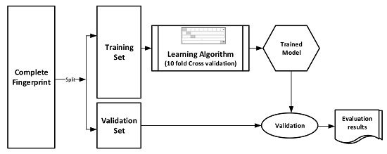
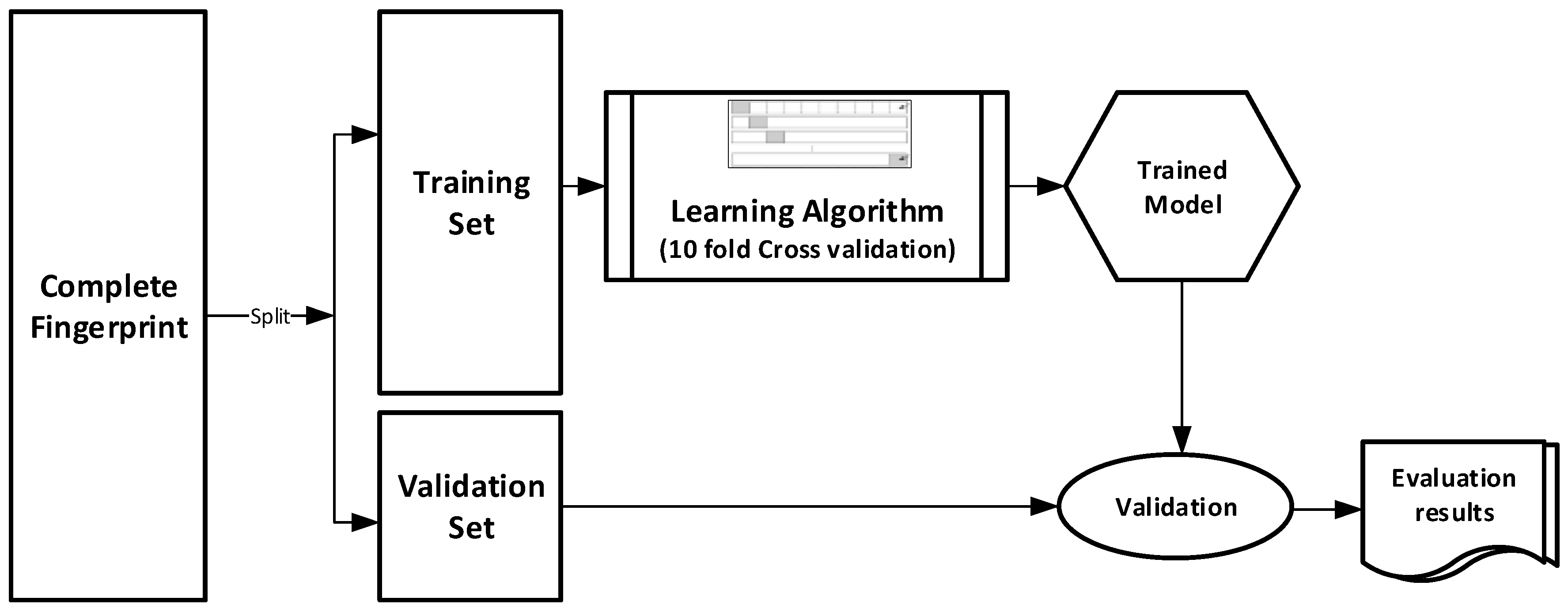
The datasets were divided into training (70%) and validation (30%) sets for the purpose of this experiment. Ten-fold cross-validation was used for the Training set. In this cross-validation, the data set was split into 10 parts; 9 were used for training and the remaining 1 was used for testing. This process is repeated 10 times with a different 10th of the dataset used to test the remaining 9 parts during every run of the 10-fold cross validation. Figure 1 pictorially illustrates the various stages involved in the work under study.

3.2. Xgboost and Machine Learning Algorithms Parameters

Identifying the optimal parameters for a classifier can be time consuming and tedious and Xgboost is not an exception. This is even more challenging in Xgboost due to the wide range of tuneable parameters for optimal performance; a few of which, using the R [28] implementation of Xgboost, we have restricted our scope to in this work. Thus, by using brute force, we obtained the best performance for Xgboost when eta, gamma, minimum child weight and maximum depth were 0.2, 0.16, 5 and 16 respectively. Where; eta is the step size shrinkage meant to control the learning rate and over-fitting through scaling each tree contribution, gamma is the minimum loss reduction required to make a split, minimum child weight is the minimum sum of instance weight needed in a child and max depth is the maximum depth of a child. Other tree booster parameters like maximum delta step, subsample, column sample and the number of trees to grow per round are left at their default values of 1 respectively. For LSVM, WEKA workbench offers a way to automate the search for optimal parameters. By using grid search, a peak performance with the radial basis kernel was obtained when gamma and cost were 5.01187233627273 × 10⁴ and 20 respectively. RF performed best when the maximum depth of tree was not constrained and the number of iteration set to its default value of 100. The NB classifier achieved best performance when kernel estimator parameter is used instead of normal distribution. For RBFN, we converted numeric attributes to nominal and set the minimum standard deviation to 0.1 to get the best performance.

3.3. Evaluation Metrics

The choice of performance evaluation for both model building and validation have been carefully selected from the most commonly used metrics in the literature. The selected evaluation metrics includes the accuracy, area under curve (AUC), sensitivity (SEN), specificity (SPC) and F-measure (F-Sc). The one run definition of AUC (Equation (11)) also known as balanced accuracy which is given by the average of the sum of sensitivity and specificity has been used in this work.
AUC = ((SEN + SPC))/2
while sensitivity (SEN) (Equation (12)) and specificity (SPC) (Equation (13)) show the ability of the model to correctly classify true positive as positive and true negative as negative respectively, AUC simply describes the tradeoff between them.
SEN = tp/(tp + fn)
SPC = tn(tn + fp)
where tp, tn, fp and fn are true positive, true negative, false positive and false negative respectively. In addition to the accuracy (Equation (14)) which is the sum of the correctly classified divided by the total number of classes, F-measure (FSc) (Equation (15)), which is the harmonic mean of precision and recall is included to serve as measure the model’s accuracy.
ACC = ((tp + tn)/(tp + tn + fn + fp))
F Sc = 2 (precision × recall)/(precision + recall)
This work aims to introduce Xgboost for activity prediction through its performance on known datasets in drug discovery. To achieve this aim, the performance of Xgboost was compared with four state of the art machine learning algorithms used in drug discovery based on the afore-stated evaluation metrics. The prediction performances of the different machine learning algorithms on the datasets under study are tabulated in Table 6, Table 7, Table 8, Table 9, Table 10, Table 11 and Table 12. The best values for each metric is shaded.
The classification performance of the MDDR1-3, DUD, COX2, BZR and ER datasets are reported in Table 6, Table 7, Table 8, Table 9, Table 10, Table 11 and Table 12 respectively.
The experimental results on MDDR1-3 Validation datasets (Table 6, Table 7 and Table 8) shows that Xgboost produced the best accuracy, sensitivity, specificity, AUC and F-Sc across all the activity classes compared to the other machine learning methods (RF, LSVM, RBFN and NB) despite the obvious imbalance distribution of activity classes in the most of the datasets. Hence, the Xgboost method performed well for the high diverse dataset (MDDR3), and these results are particularly interesting since the MDDR3 is made up of heterogeneous activity classes which are more challenging for most machine learning algorithms.
For DUD Validation dataset (Table 9), Xgboost and RF produced the best accuracy (0.9471) compared to the other methods. In addition, Xgboost produced the best specificity across all DUD sub datasets. However, NB obtained the best sensitivity, AUC and F-Sc results.
For COX2, ER and BZR Validation datasets (Table 10, Table 11 and Table 12), it is shown that Xgboost performed well and produced the best accuracy and AUC for COX2 and ER datasets. In addition, it obtained the best F-Sc results for COX2 dataset compared to the other state-of-art methods.
Visual inspection of the results shows that Xgboost produced the best accuracy for all used datasets (except for BZR dataset which produced the second best accuracy). While the performance of Xgboost on most activity classes in terms of accuracy and AUC remains the best, it still produces the best average performance across all evaluation metrics. In addition, the good performance of Xgboost is not only restricted to homogenous activity classes since it also performed well on the heterogeneous dataset.
Moreover, a quantitative approach using Kendall W test of concordance was used to rank the effectiveness of all used methods as shown in Table 13. This test shows whether a set of raters make comparable judgments on the ranking of a set of objects. Hence, the XGB, RF, LSVM, RBFN and NB methods were used as the raters, and the accuracy measure (using MDDR1-3, DUD, COX2, BZR and ER datasets respectively) were used as the ranked objects. The outputs of this test are the Kendall coefficient (W) and the associated significance level (p value). In this paper, if the value is significant at a cutoff value of 0.01, then it is possible to give an overall ranking for the methods.
The results of the Kendall analysis for the seven datasets are shown in Table 13. The columns show the evaluation measure, the value of the Kendall coefficient (W), the associated significance level (p value), and the ranking of prediction methods. The overall rankings of the four methods show that Xgboost significantly outperforms the other methods using accuracy measure across all datasets.

4. Conclusions

This paper investigated the performance of Xgboost on bioactivity prediction and found out that Xgboost is indeed a robust predictive algorithm. Experimental results show that Xgboost is not only effective as a predictive model for homogeneous dataset but can replicate such effectiveness on structurally heterogeneous dataset. Experimental results show that Xgboost produces an impressive predictive accuracy, ranging from 94.47% accuracy in the heterogeneous data to 98.49% in the homogeneous one. In addition to the obvious fact that Xgboost has been shown in this work to be a good predictive tool for bioactive molecule, we are hopeful that by this Xgboost would be seen as an invaluable addition to already known computational approaches to target prediction and thus leading to a wider perspective of the data rather than a single approach.

Acknowledgments

This work is supported by the Ministry of Higher Education (MOHE) and Research Management Centre (RMC) at the Universiti Teknologi Malaysia (UTM) under the Research University Grant Category (VOT Q.J130000.2528.14H75).

Author Contributions

I.M. is a researcher and conducted this project research under the supervision of F.S. All authors read and approved the final manuscript.

Conflicts of Interest

The authors declare no conflict of interest.

References

  1. Johnson, M.A.; Maggiora, G.M. Concepts and Applications of Molecular Similarity; John Wiley & Sons: New York, NY, USA, 1990. [Google Scholar]
  2. Wassermann, A.M.; Geppert, H.; Bajorath, J. Searching for target-selective compounds using different combinations of multiclass support vector machine ranking methods, kernel functions, and fingerprint descriptors. J. Chem. Inf. Mod. 2009, 49, 582–592. [Google Scholar] [CrossRef] [PubMed]
  3. Yang, Z.R. Biological applications of support vector machines. Brief. Bioinform. 2004, 5, 328–338. [Google Scholar] [CrossRef] [PubMed]
  4. Deconinck, E.; Zhang, M.H.; Coomans, D.; Vander Heyden, Y. Classification tree models for the prediction of blood-brain barrier passage of drugs. J. Chem. Inf. Mod. 2006, 46, 1410–1419. [Google Scholar] [CrossRef] [PubMed]
  5. Svetnik, V.; Liaw, A.; Tong, C.; Culberson, J.C.; Sheridan, R.P.; Feuston, B.P. Random Forest:  A Classification and Regression Tool for Compound Classification and QSAR Modeling. J. Chem. Inf. Comput. Sci. 2003, 43, 1947–1958. [Google Scholar] [CrossRef] [PubMed]
  6. Kauffman, G.W.; Jurs, P.C. QSAR and k-nearest neighbor classification analysis of selective cyclooxygenase-2 inhibitors using topologically-based numerical descriptors. J. Chem. Inf. Comput. Sci. 2001, 41, 1553–1560. [Google Scholar] [CrossRef] [PubMed]
  7. Koutsoukas, A.; Lowe, R.; KalantarMotamedi, Y.; Mussa, H.Y.; Klaffke, W.; Mitchell, J.B.; Glen, R.C.; Bender, A. In silico target predictions: Defining a benchmarking data set and comparison of performance of the multiclass naïve bayes and parzen-rosenblatt window. J. Chem. Inf. Mod. 2013, 53, 1957–1966. [Google Scholar] [CrossRef] [PubMed]
  8. Krenker, A.; Kos, A.; Bešter, J. Introduction to the Artificial Neural Networks; INTECH Open Access Publisher: Rijeka, Croatia, 2011. [Google Scholar]
  9. Lavecchia, A. Machine-learning approaches in drug discovery: Methods and applications. Drug Discov. Today 2015, 20, 318–331. [Google Scholar] [CrossRef] [PubMed]
  10. Wolpert, D.H. The supervised learning no-free-lunch theorems. In Soft Computing and Industry; Springer: London, UK, 2002; pp. 25–42. [Google Scholar]
  11. Friedman, J.H. Greedy function approximation: A gradient boosting machine. Ann. Stat. 2001, 29, 1189–1232. [Google Scholar] [CrossRef]
  12. Adam-Bourdarios, C.; Cowan, G.; Germain-Renaud, C.; Guyon, I.; Kégl, B.; Rousseau, D. The Higgs Machine Learning Challenge. J. Phys. Conf. Ser. 2015. [Google Scholar] [CrossRef]
  13. Phoboo, A.E. Machine Learning wins the Higgs Challenge. CERN Bull. 2014. Available online: http://cds.cern.ch/journal/CERNBulletin/2014/49/News%20Articles/1972036 (accessed on 24 April 2016). [Google Scholar]
  14. Harper, G.; Bradshaw, J.; Gittins, J.C.; Green, D.V.; Leach, A.R. Prediction of biological activity for high-throughput screening using binary kernel discrimination. J. Chem. Inf. Comput. Sci. 2001, 41, 1295–1300. [Google Scholar] [CrossRef] [PubMed]
  15. Chen, T.; Guestrin, C. Xgboost: A Scalable Tree Boosting System. arXiv:1603.02754 2016. [Google Scholar] [CrossRef]
  16. Chang, C.-C.; Lin, C.-J. LIBSVM: A library for support vector machines. ACM Trans. Intell. Syst. Technol. 2011, 2, 27. [Google Scholar] [CrossRef]
  17. John, G.H.; Langley, P. Estimating Continuous Distributions in Bayesian Classifiers. In Proceedings of the Eleventh Conference on Uncertainty in Artificial Intelligence, Montreal, QC, Canada, 18–20 August 1995.
  18. Bugmann, G. Normalized Gaussian radial basis function networks. Neurocomputing 1998, 20, 97–110. [Google Scholar] [CrossRef]
  19. Sutherland, J.J.; O’Brien, L.A.; Weaver, D.F. Spline-Fitting with a Genetic Algorithm: A Method for Developing Classification Structure−Activity Relationships. J. Chem. Inf. Comput. Sci. 2003, 43, 1906–1915. [Google Scholar] [CrossRef] [PubMed]
  20. Helma, C.; Cramer, T.; Kramer, S.; de Raedt, L. Data Mining and Machine Learning Techniques for the Identification of Mutagenicity Inducing Substructures and Structure Activity Relationships of Noncongeneric Compounds. J. Chem. Inf. Comput. Sci. 2004, 44, 1402–1411. [Google Scholar] [CrossRef] [PubMed]
  21. Huang, N.; Shoichet, B.K.; Irwin, J.J. Benchmarking sets for molecular docking. J. Med. Chem. 2006, 49, 6789–6801. [Google Scholar] [CrossRef] [PubMed]
  22. Al-Dabbagh, M.M.; Salim, N.; Himmat, M.; Ahmed, A.; Saeed, F. A Quantum-Based Similarity Method in Virtual Screening. Molecules 2015, 20, 18107–18127. [Google Scholar] [CrossRef] [PubMed]
  23. Cross, S.; Baroni, M.; Carosati, E.; Benedetti, P.; Clementi, S. FLAP: GRID molecular interaction fields in virtual screening. Validation using the DUD data set. J. Chem. Inf. Mod. 2010, 50, 1442–1450. [Google Scholar] [CrossRef] [PubMed]
  24. BIOVIA. MDDR. Retrieved 15–07, 2015. Available online: http://accelrys.com/products/databases/bioactivity/mddr.html (accessed on 15 July 2015).
  25. Abdo, A.; Saeed, F.; Hamza, H.; Ahmed, A.; Salim, N. Ligand expansion in ligand-based virtual screening using relevance feedback. J. Comput. Aided Mol. Design 2012, 26, 279–287. [Google Scholar] [CrossRef] [PubMed]
  26. Abdo, A.; Leclère, V.; Jacques, P.; Salim, N.; Pupin, M. Prediction of New Bioactive Molecules using a Bayesian Belief Network. J. Chem. Inf. Model. 2014, 54, 30–36. [Google Scholar] [CrossRef] [PubMed]
  27. Hert, J.; Willett, P.; Wilton, D.J.; Acklin, P.; Azzaoui, K.; Jacoby, E.; Schuffenhauer, A. New methods for ligand-based virtual screening: Use of data fusion and machine learning to enhance the effectiveness of similarity searching. J. Chem. Inf. Mod. 2006, 46, 462–470. [Google Scholar] [CrossRef] [PubMed]
  28. The R Core Team. R: A Language and Environment for Statistical Computing; R Foundation for Statistical Computing: Vienna, Austria, 2013. [Google Scholar]
  • Sample Availability: Not Available.
Figure 1. Experimental Design.
Molecules 21 00983 g001
Table 1. Activity Classes for cyclooxygenase-2 (COX2) estrogen receptor (ER) and benzodiazepine receptor (BZR) Datasets.
DatasetsNumber of CompoundsPairwise Similarity (Mean)
ActiveInactiveActiveInactive
TrainingValidationTrainingValidation
Cyclooxygenase-2 inhibitors21192116480.6870.690
Benzodiazepine receptor2149270290.5360.538
Estrogen receptor8655190620.4680.456
Table 2. Number of Active (Na) compounds for 12 Directory of Useful Decoys (DUD) datasets.
NoActivity ClassNa
TrainingValidation
1FGFR1T9030
2FXA10640
3GART2713
4GBP3814
5GR5523
6HIVPR4220
7HIVRT3211
8HMGA2411
9HSP902413
10MR105
11NA3514
12PR225
Table 3. Activity Classes for MDDR1.
Activity IndexActivity ClassActive MoleculesPairwise Similarity
TrainingValidationMean
31420renin inhibitors7833470.573
71523HIV protease inhibitors5352150.446
37110thrombin inhibitors5612420.419
31432angiotensin II AT1 antagonists6742690.403
42731substance P antagonists8593870.339
062335HT3 antagonists5302220.351
062455HT reuptake inhibitors2571020.345
07701D2 antagonists2681270.345
062355HT1A agonists5892380.343
78374protein kinase C inhibitors3261270.323
78331cyclooxygenase inhibitors4272090.268
Table 4. Activity Classes for MDDR2.
Activity IndexActivity ClassActive MoleculesPairwise Similarity
TrainingValidationMean
07707adenosine (A1) agonists136710.424
07708adenosine (A2) agonists119370.484
31420renin inhibitors7913390.584
42710monocyclic β-lactams78330.596
64100cephalosporins9113900.512
64200carbacephems115430.503
64220carbapenems7323190.414
64300penicillin88380.444
65000antibiotic, macrolide2681200.673
75755vitamin D analogous3231320.569
Table 5. Activity Classes for MDDR3.
Activity IndexActivity ClassActive MoleculesPairwise Similarity
TrainingValidationMean
09249muscarinic (M1) agonists6202800.257
12455NMDA receptor antagonists9904100.311
12464nitric oxide synthase inhibitors3481570.237
31281dopamine β-hydroxylase inhibitors76300.324
43210aldose reductase inhibitors6632940.37
71522reverse transcriptase inhibitors5011990.311
75721aromatase inhibitors4441920.318
78331cyclooxygenase inhibitors4491870.382
78348phospholipase A2 inhibitors4301870.291
78351lipoxygenase inhibitors14786330.365
Table 6. Sensitivity, Specificity, Area under Curve, Accuracy and F-measure on MDDR1 Dataset.
ML AlgorithmTrainingValidation
SENSPCAUCACCF-ScSENSPCAUCACCF-Sc
XGB0.94840.99580.97210.95750.98300.95790.99600.97690.95940.9536
RF0.94740.99630.97180.96210.95140.95020.99570.97300.95900.9525
LSVM0.92580.99430.96000.94250.92640.93570.99480.96530.94970.9371
RBFN0.75660.97730.86700.77190.74510.77510.97770.87640.77460.7553
NB0.76480.97810.87150.78260.75780.74880.97620.86250.76260.7383
Table 7. Sensitivity, Specificity, Area under Curve, Accuracy and F-measure on MDDR2 Dataset.
ML AlgorithmTrainingValidation
SENSPCAUCACCF-ScSENSPCAUCACCF-Sc
XGB0.97790.99810.98800.98340.96890.98200.99830.99020.98490.9673
RF0.95620.99790.97710.98370.96890.94680.99770.97230.98230.9597
LSVM0.95900.99780.97840.98170.96670.94360.99740.97050.97900.9547
RBFN0.95070.99610.97349.96460.94020.94200.99600.96900.96580.9312
NB0.95460.99630.97550.96770.94580.94010.99670.96840.97240.9403
Table 8. Sensitivity, Specificity, Area under Curve, Accuracy and F-measure on MDDR3 Dataset.
ML AlgorithmTrainingValidation
SENSPCAUCACCF-ScSENSPCAUCACCF-Sc
XGB0.94070.99370.96720.94400.93480.94930.99370.97150.94470.9448
RF0.92090.99290.956994.0990.93500.93160.99280.96220.93970.9405
LSVM0.88000.98850.9342590.46510.89480.89830.99020.94430.91710.9120
RBFN0.70530.96430.834868.06130.65970.72540.96570.84560.68900.6710
NB0.68030.96130.820865.72760.64020.66360.95940.81150.64150.6211
Table 9. Sensitivity, Specificity, Area under Curve, Accuracy and F-measure on DUD Dataset.
ML AlgorithmTrainingValidation
SENSPCAUCACCF-ScSENSPCAUCACCF-Sc
XGB0.86770.99200.92980.91130.86160.85690.99530.92610.94710.8673
RF0.88610.99350.93970.92940.89080.90780.99510.95150.94710.9123
LSVM0.86590.99190.92890.91130.86830.87380.99410.93400.93750.8862
RBFN0.82280.98950.90610.88710.83440.85030.99310.92170.92790.8537
NB0.87830.99100.93460.90320.87300.91770.99420.95590.93750.9193
Table 10. Sensitivity, Specificity, Area under Curve, Accuracy and F-measure on COX2 Dataset.
ML AlgorithmTrainingValidation
SENSPCAUCACCF-ScSENSPCAUCACCF-Sc
XGB0.93610.94440.94030.93880.95350.95700.93620.94660.95000.9622
RF0.97630.88790.93210.94500.95810.97830.87500.92660.94290.9574
LSVM0.95260.91380.93320.93880.95260.95650.89580.92620.93570.9514
RBFN0.92930.72030.82480.83790.86580.92500.70000.81250.82860.8605
NB0.67770.95690.81730.77680.79670.70651.00000.85330.80710.8280
Table 11. Sensitivity, Specificity, Area under Curve, Accuracy and F-measure on BZR Dataset.
ML AlgorithmTrainingValidation
SENSPCAUCACCF-ScSENSPCAUCACCF-Sc
XGB0.97640.90280.93960.95770.97180.98840.80000.89420.93390.9551
RF0.97200.91430.94310.95770.97200.96740.89660.93200.95040.9674
LSVM0.95790.87140.91470.93660.95790.93481.00000.96740.95040.9663
RBFN0.99470.72630.86050.90490.93301.00000.64440.82220.86780.9048
NB0.91120.85710.88420.89790.93080.84780.96550.90670.87600.9123
Table 12. Sensitivity, Specificity, Area under Curve, Accuracy and F-measure on ER Dataset.
ML AlgorithmTrainingValidation
SENSPCAUCACCF-ScSENSPCAUCACCF-Sc
XGB0.76710.85220.80970.82970.70440.88370.77030.82700.81200.7755
RF0.68600.88950.78780.82610.71080.63640.82260.72950.73500.6931
LSVM0.66280.93160.79720.84780.73080.67270.91940.79600.80340.7629
RBFN0.70890.84770.77830.80800.67880.84780.77460.81120.80340.7723
NB0.97670.63680.80680.74280.70290.98180.56450.77320.76070.7941
Table 13. Rankings of Prediction Methods based on Kendall W Test Using Accuracy Measure.
MeasureWPRanks
Accuracy0.650.001XGBOOST > RF > LSVM > RBFN > NB

