2. Materials and Methods
2.1. The Method
The smooth changes of average daily flow rates and water levels throughout the year, typical for fairly large rivers, provide the basis for the simplest version of flow forecasting by extrapolating the hydrograph. Such extrapolation can provide the forecast of the average daily water discharge with the lead-time
days in the form of a generalized polynomial:
where
is the streamflow forecast,
,
, …,
—coefficients described below;
,…,
are some predefined functions. For example, in the case of
,…,
, Formula (1) means the extrapolation of the hydrograph to
days ahead by polynomials to the power of
. In particular, for a value of
, a linear extrapolation is performed, and for a value of
, a parabolic extrapolation is performed. Depending on the forecast date
, values
,
, …,
in the Formula (1) are determined based on the assumption that the sequence of observed discharges
,
, …,
for the forecast date and for
previous days are described by the same generalized polynomial. This assumption is expressed as a system of equations:
The solution of the system (2) leads to linear expression of the values
,
, ….,
in terms of discharges
,
, …,
. After substituting these expressions into Formula (1), it takes the form:
Thus, the extrapolation of the hydrograph using any polynomial of the Formula (1) leads to the fact that the forecast is expressed as a linear combination of the corresponding date of the forecast of water discharge and previous discharges , …, .
The values determined by Formula (3) can take extremely and unrealistic high and low values. Extremely high values can occur when predicting water discharges on a steep rise of streamflow during spring floods or rainfall induced floods. Extremely low and even negative values can occur when forecasting water discharges and water levels during a steep spring flood or rain flood recession period.
In order to avoid unrealistically low and high forecast values, the results of Formula (3) application shall be adjusted by replacing such extreme values
with acceptable minimum
or acceptable maximum
discharge values. The final scheme of water discharge forecast is expressed by the formula:
The generalized extrapolation of the average daily water levels leads to a similar formula, which expresses the forecast of the water level
in the form of a linear combination of the average daily level known by the date of the forecast
and
levels
,…,
for the previous days:
The results of applying Formula (5) are adjusted in the same way by replacing the extreme values
with an acceptable minimum
or maximum
values of water level. The final forecast scheme of water level is expressed by the formula:
Limiting the permissible values of streamflow rates and water levels using Formulas (4) and (6) allows one to avoid unnecessarily low and high flow rates. However, in this case, there is a danger of underestimating the expected extreme characteristics of the river streamflow. In order to reduce the likelihood of such an underestimation, an estimate of a quantile corresponding to close to 100% of the annual probability of exceeding, for example, 99%, should be used as an acceptable minimum. An estimate of the quantile corresponding to a near 0% annual probability of exceeding, for example, 1%, should be used as an acceptable maximum.
This method is a variant of the Wiener filter, which is widely used in various branches of science [
13,
14]. The method can be also considered as a particular option of the forecast correction scheme which takes into account the autocorrelation of their errors [
15].
It is not absolutely robust, since it requires a statistical assessment of the parameters of Formulas (3) and (4) or (5) and (6). However, when using a sufficient amount of data over a long period, the estimates of these parameters can be quite stable.
The method can be used for short- or medium-term forecasting of river runoff and water level during a certain phase of the water regime or throughout the year. It is not purely formal, since the water discharge and water levels taken into account in Formulas (3) and (5) for
days indirectly characterize the flow of meltwater or rainwater, the replenishment or depletion of soil moisture and groundwater reserves, the change in riverbed and floodplain water reserves, and the transformation of a spring flood wave or rain flood during the previous period. The possibilities of using this method are confirmed by its sufficiently successful application for obtaining short-term forecasts of river runoff in the Kama river basin [
16].
2.2. Implementation
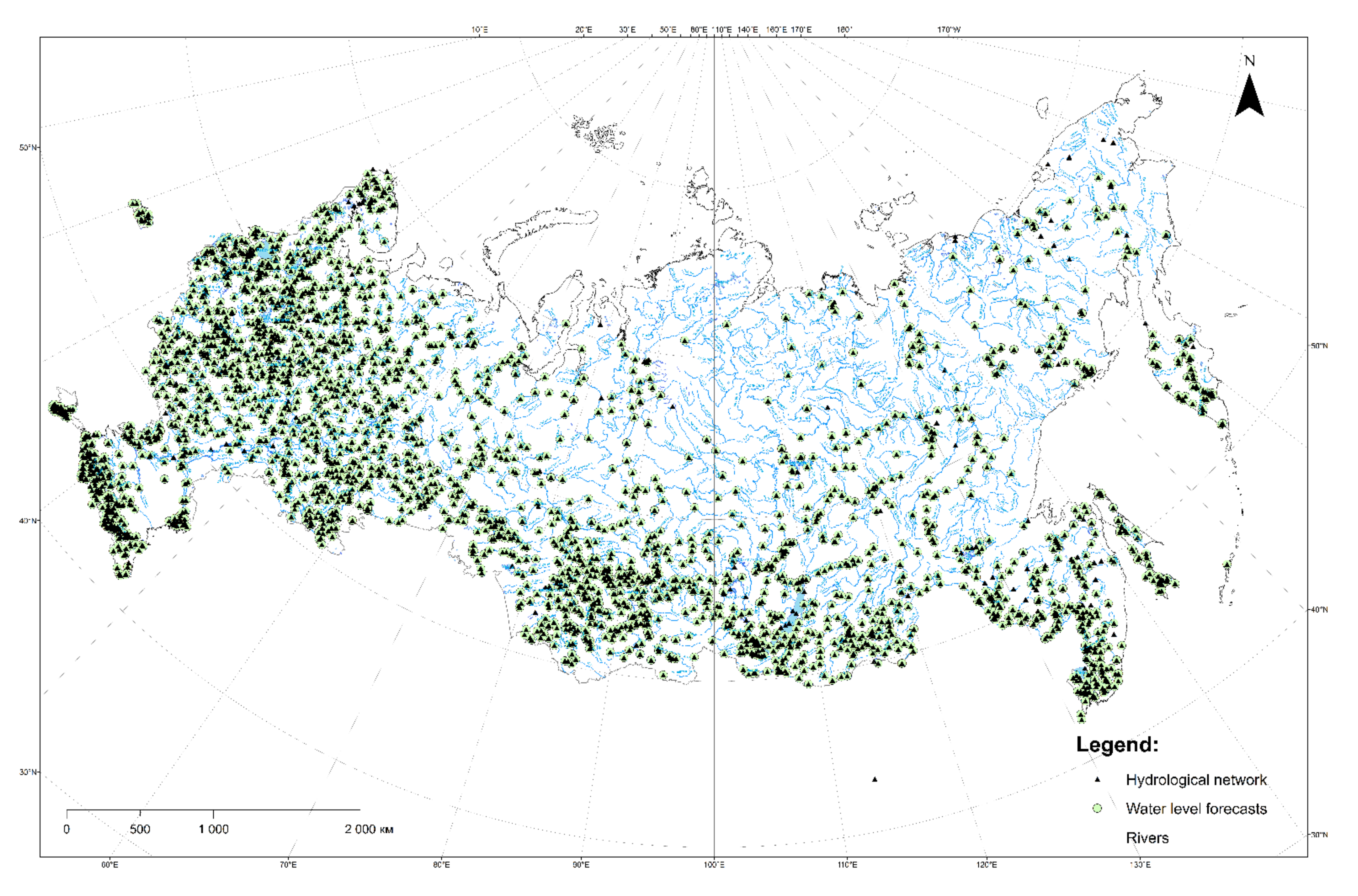
The hydrograph extrapolation method was used to predict the average daily discharge and water levels at stream gauging stations across Russia throughout the year. The method for daily water level forecasting was applied at 2776 gauges, for discharge forecasting—for 2098 stream gauging stations (
Figure 1). In each case, a continuous time series of daily hydrological observations was used to develop the method for the period from 1 January 2010 to 31 December 2019.
For a given forecast lead time = 1, …, 10 the parameters , ,…, and used in Formula (3) or (5) were estimated by the least square method. The minimum and maximum values of discharges and water levels included in Formulas (4) and (6) were determined from the long-term series of hydrological observations.
For each value of the lead-time from 1 to 10 days, the optimal number was selected for Formulas (3) and (5), at which the value of forecast root-mean-square error is minimal. The analysis showed that for all values of the forecast lead-time = 1, …, 10, the values of such optimal parameter did not exceed 5. On this basis, all forecasts of average daily discharges and water levels were determined according to the Formulas (3) and (5) using = 5.
As permissible minima and maxima of river runoff in Formulas (4) and (6), estimates of quantiles corresponding to the annual probability of exceeding 99% and 1% were used, obtained for the entire period of long-term observations available for each river section.
As an example,
Table 1 indicates values of parameters of Formulas (3) and (4) for generating forecasts of the average daily water discharges of the Don River near Serafimovich with a lead time
= 1, …, 10 days.
In order to automate the procedure for generating forecasts and quality assessment for any set of gauging stations, a computer program was developed using Python programming language and set up in the Hydrometcenter of Russia. The computer program includes the following steps:
- ―
reading and processing data that can be stored in one or more files;
- ―
estimation of the parameters of the forecast scheme for each gauging station;
- ―
evaluation of various indicators of the received forecasts quality;
- ―
creating a separate directory for each gauge, where the parameters of the forecast generation scheme and its quality indicators are stored;
- ―
creating the result table with forecasts.
2.3. Forecasts Verification
The quality of short- and medium-term forecasts of average daily discharges and water levels was evaluated based on an independent data sample that was not taken into account when determining the parameters of the forecast formulas. For this purpose, the jackknife approach was applied [
17,
18]:
- (1)
first year was excluded from the 10-year observation period;
- (2)
data for the remaining 9 years were used to estimate the parameters of the forecast generation scheme;
- (3)
resulting estimates were substituted into Formulas (3) and (4) or (5) and (6) to predict discharges or water levels during the excluded year;
- (4)
for the excluded year (independent sample), a series of forecast errors for 365 or (for a leap year) 366 days was formed;
- (5)
data for the excluded first year were returned and the next year excluded;
- (6)
data for the second year were excluded on the next step of cross-validation;
- (7)
after repeating the described procedure for all 10 years, an -long series of forecast errors, obtained on an independent material, was formed ( = 3652).
The check performed in this way showed that when using the data of daily observations for 10 years, the parameters of the formulas for obtaining the forecast are quite stable, since their estimates practically coincided for each of the 10 options for excluding data for one of 10 years.
If we denote the average value of the predicted value per day
by
and its forecast by
, then for the period from 1 January 2010 to 31 December 2019, the Nash–Sutcliffe model efficiency coefficient is determined by the formula:
where
is the arithmetic mean of the series
, …,
of the actual values of the modeled characteristic [
18]. This indicator does not exceed 1; moreover, the equality
is achieved for an absolutely exact model that ensures the coincidence of the quantities
and
. Equality
means that modeling is as accurate as calculating a quantity
from its mean
. Negative
values indicate completely unsatisfactory simulation results.
The paper [
15] proposes the following classification of the quality of models: a model can be considered good if
; satisfactory provided
; unsatisfactory provided
.
For all river sections and flow characteristics, the average forecast error − is zero, that is, the extrapolation of the hydrograph does not give systematic forecast errors.
For the forecast of the Don River daily streamflow near Serafimovich, lead times varying from 1 to 10 days,
values are presented in
Table 2.
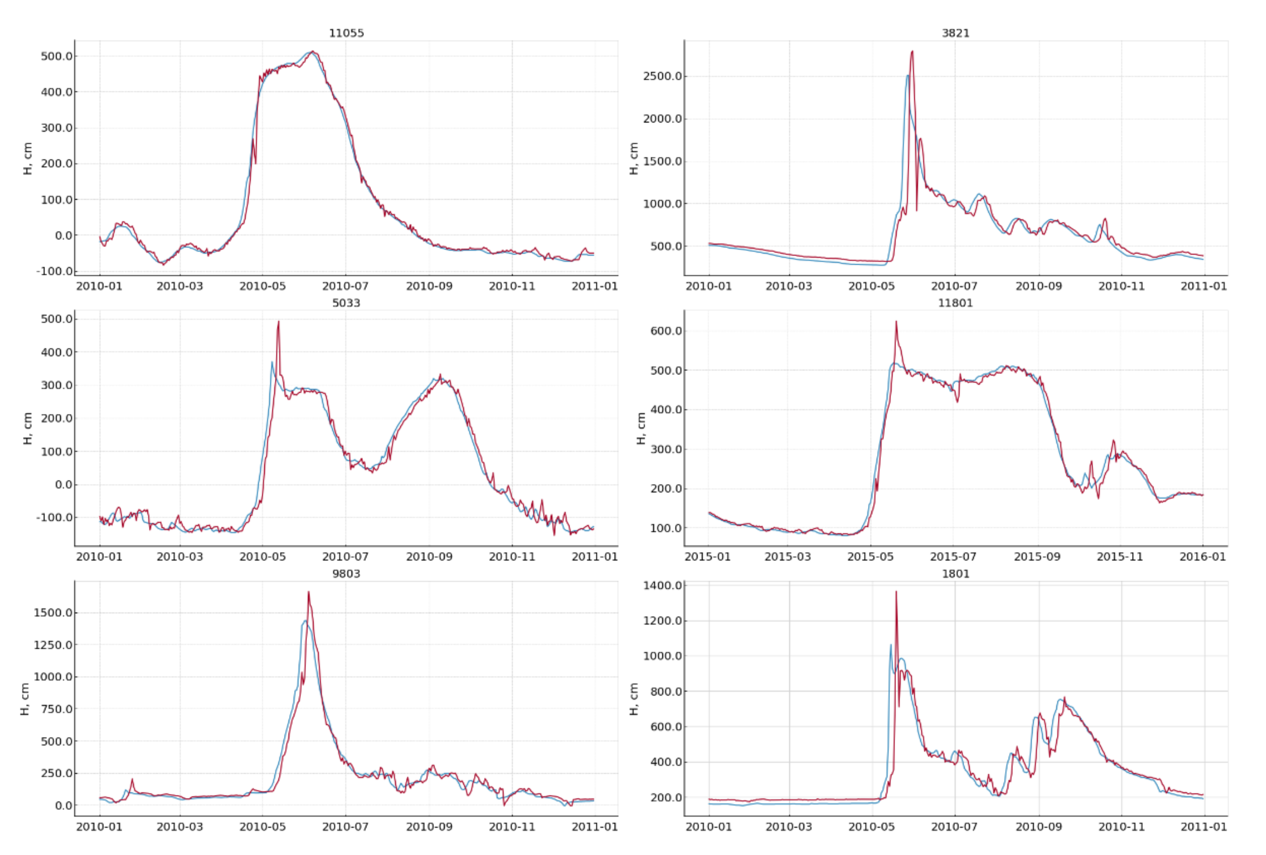
Figure 2 shows observed and forecasted hydrographs at major gauging stations in 2010–2011; streamflow forecast lead-time is 5 days.
3. Results
For the stream gauging stations across Russia, the results of streamflow and water level forecast verification make it possible to assess the performance of the used method of hydrograph extrapolation and the automated system of forecast preparation and issuance.
The number of gauging stations where satisfactory or good forecasts (NSE ≥0.36) of discharges Q, m
3/s, and water level H, cm have been achieved using the technique is given in
Table 3.
The data in this table show that with lead time = 1 day, satisfactory forecasts of water discharge can be obtained for 2069 gauging stations, satisfactory forecasts of water levels for 2775 stations; with lead time = 2 days, for 2015 and 2769 stations, respectively, etc. At the same time, the stations for which satisfactory forecasts were obtained with a longer lead time are also included in the number of stations with satisfactory forecasts with lead time .
It is important that with maximum lead time for medium-term forecasts = 10 days, water discharges are forecasted satisfactorily for 1008 gauging stations and water levels for 2237 stations.
Table 4 shows the numbers of stream gauging stations where flow and water level forecasts were good for lead times from 1 to 10 days (efficiency coefficient not less than 0.8).
Information given in
Table 3 and
Table 4 demonstrates that in general, water levels are better forecasted than discharges using the technique. This is due to the significantly higher amplitude of fluctuations of discharge and thus, the less smooth change in time.
In addition, for every lead time, the number of gauging stations with satisfactory flow forecasts significantly exceeds the corresponding number with good forecasts.
Generally, the accuracy of the hydrograph extrapolation method turned out to be lower for rivers with a small catchment area and large watershed slope, in particular, for small mountain rivers. This is due to the fact that under such conditions, river runoff responds quickly (sometimes it takes a few hours) to snow melting or rainfall [
2,
7,
18]. As a result, the water regime is determined by a series of short-term floods, outside of the winter low-water period, one can speak of a saw-tooth flow hydrograph, and it is difficult to predict this with sufficient accuracy even for the next day. For such rivers, it is necessary to use methods that are based on modeling the processes of river runoff. Due to this, an automated system for preparing and issuing short-term forecasts of small Russian rivers runoff is being developed in the present time; it is based on conceptual models of river runoff formation including the Hydrometcenter of the Russia model and the Swedish HBV model [
8,
19].
The change of average daily water discharge and levels is smooth, as in
Figure 2, for rivers with big catchment area and small watershed slope; therefore, the hydrograph extrapolation method allows satisfactory and good forecasts to be made with a sufficiently long lead-time. This method gives good forecasts with lead time up to 10 days for such large Russian rivers as the Amur, Lena, Yenisey, Ob, Irtysh, Tobol, Kama, Don, Northern Dvina and Pechora.
The efficiency coefficient value is decreasing with an increase in the lead time of the forecast ∆t. This allows determining of the maximum lead time for good forecasts max(∆t) in such a way that forecasts with efficiency coefficient value not less than 0.8 can be obtained for all values ∆t not exceeding max(∆t).
For water discharges, the average value of maximum lead time of good forecasts is 3.3 days, and for water levels, 4.7 days. For satisfactory forecasts of water discharges and water levels, maximum lead times are 7.6 and 9.4 days, respectively.
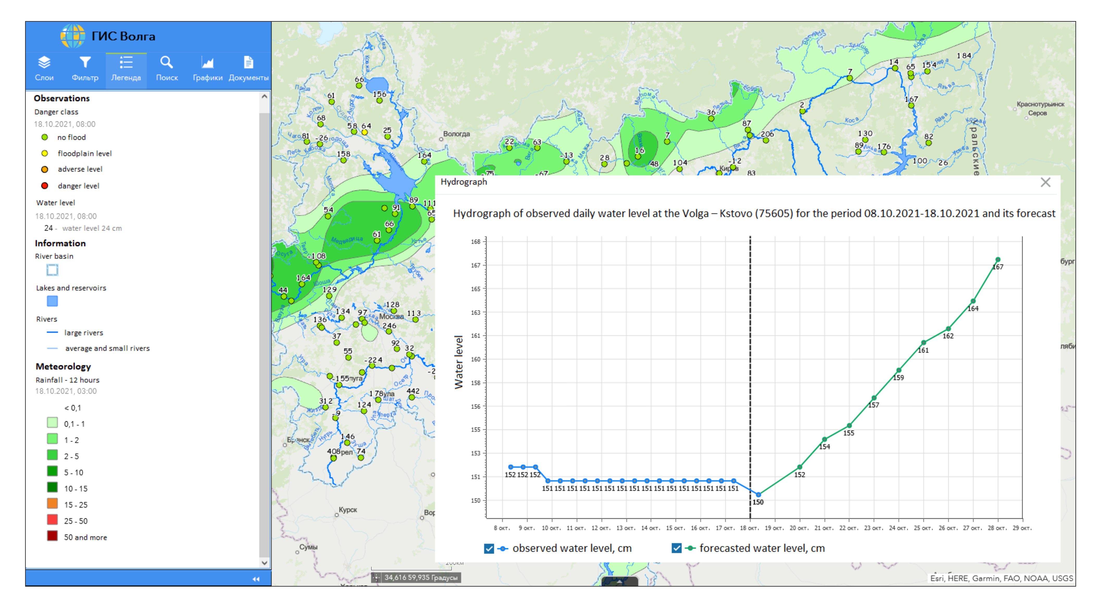
One of the most important tasks of the operational hydrological forecasting system is the forecasts provision to end users (including hydrologists at regional offices, National Disaster Management Agency, Cities administrations and others) in a timely and effective manner. For this purpose, the system for monitoring and forecasting of floods and other adverse hydrological phenomena was developed based on the recent advances of GIS-WEB technologies [
11,
19]. Forecasts of water levels, automatically issued according to the abovementioned techniques, are sent to the delivery system in the form of web services. The user, in a real time mode, using a regular web interface, has access to forecasts of flows and water levels (
Figure 3). During operation, the systems demonstrated the accuracy and reliability of forecasting, the efficiency of bringing the output products to the end users for making correct and timely decisions aimed at minimizing damage from the passage of floods.
The ability to extrapolate the hydrograph is characterized by the maximum lead time of good forecasts max(∆t) when NSE ≥ 0.80. Maximum lead time of good forecasts depends on not only the catchment area size and watershed slope but also on other natural (climate, relief, landscape) as well manmade conditions of river flow formation. Thus, defining the relation between maximum lead time max(∆t) and the catchment area and watershed slope is possible only for geographically homogeneous regions. For such areas, the smoothness of the hydrographs’ shape increases with an increase in the catchment area A and a decrease in its average slope I. Consequently, with an increase in A and a decrease in I, the maximum lead time of good forecasts max(∆t) should increase.
When identifying such regions, data on 1879 river gauges with natural river flow located throughout the entire territory of Russia were used. For each gauge, according to the data of daily observations, the maximum lead time of good forecasts max(∆t) was calculated using the hydrograph extrapolation method. The values of the watershed area A and its average slope I were obtained.
As a first approximation, the predictability indicator max(∆t) and the catchment area A and the average slope I dependence were analyzed. For this purpose, various types of the function f(A, I) were considered, for each of which the correlation coefficient r between f(A, I) and the max(∆t) was estimated. The variant of f(A, I) was chosen as the optimal one, where the coefficient r had the maximum value. The logarithm of the catchment area ln(A) turned out to be such an optimal variant. The maximum value of r appeared to be 0.50. The tightness of the max(∆t) and ln(A) dependence turned out to be insufficient for assessing the predictability of river flow in specific river sections using the values of A and I. In this regard, the search for closer dependences of the indicator max(∆t) on the optimal type of the function f(A, I) was considered for geographically homogeneous regions.
When identifying regions with a single dependence of the
max(∆
t) and the area
A and the average slope
I of the catchments, the goal was to achieve, at least, its relative geographical homogeneity. To achieve this goal, the information contained in the Big Geographical Atlas of Russia was taken into account [
18]. The procedure for identifying each region included the following steps:
identification of the “core” formed by catchments with fairly similar flow formation conditions and its regime;
preliminary identification of the optimal type of the function f(A, I), which has the maximum correlation coefficient r with the index max(∆t);
adding adjacent catchments if their data do not significantly reduce the value of r;
refinement of the optimal type of the function f(A, I);
discarding adjacent catchments if their data negatively influenced the relationship.
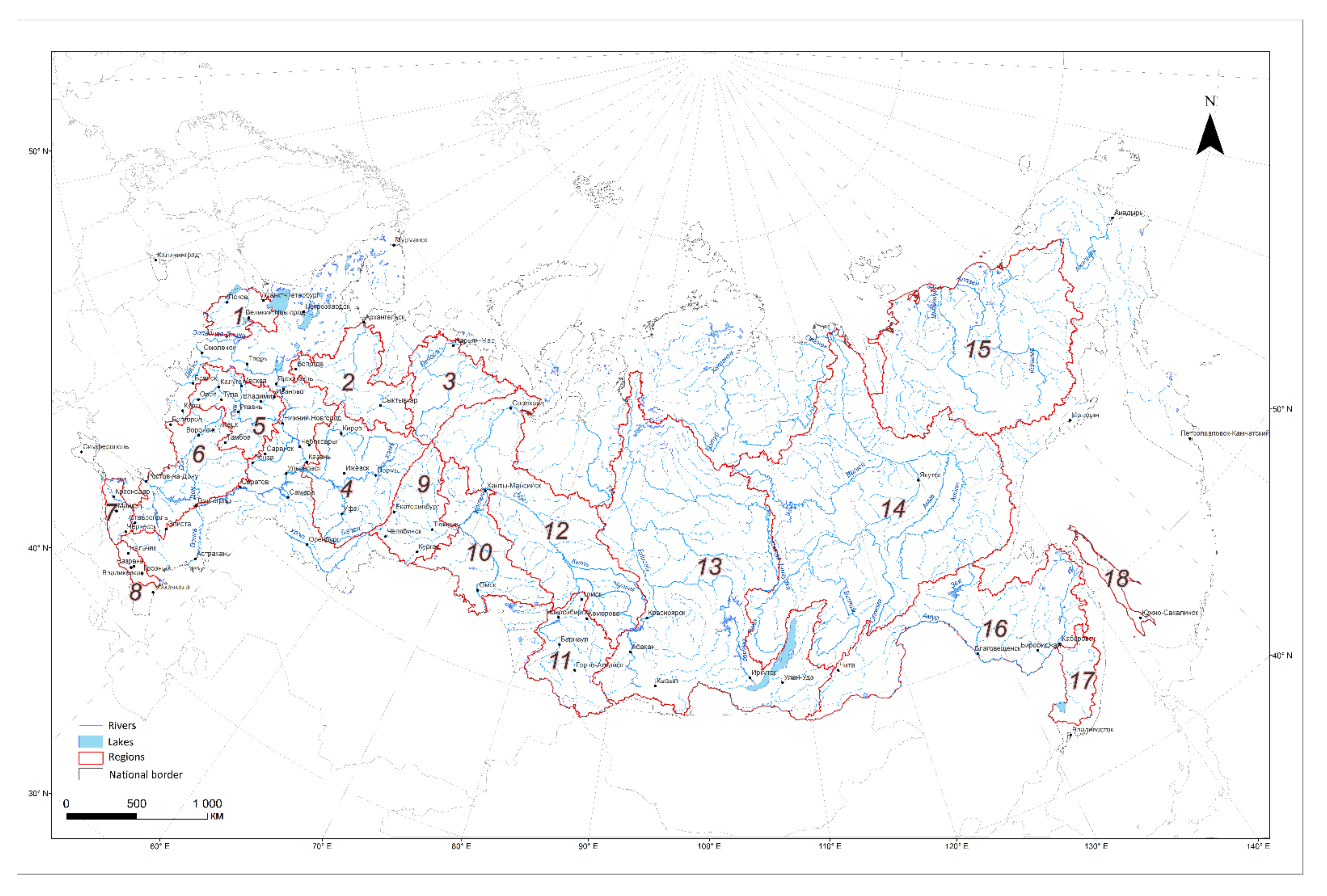
Thus, 18 regions were identified with a single dependence of the predictability indicator of river runoff
max(∆
t) on the function of morphometric characteristics of the catchment area
f(A, I) corresponding to each region. These regions cover about 80% of the entire country and are shown in
Figure 4.
Table 5 shows the name, number of river gauges N, optimal type of the function
f(A, I) and the correlation coefficient
r of the relationship with
max(∆
t) for each region.
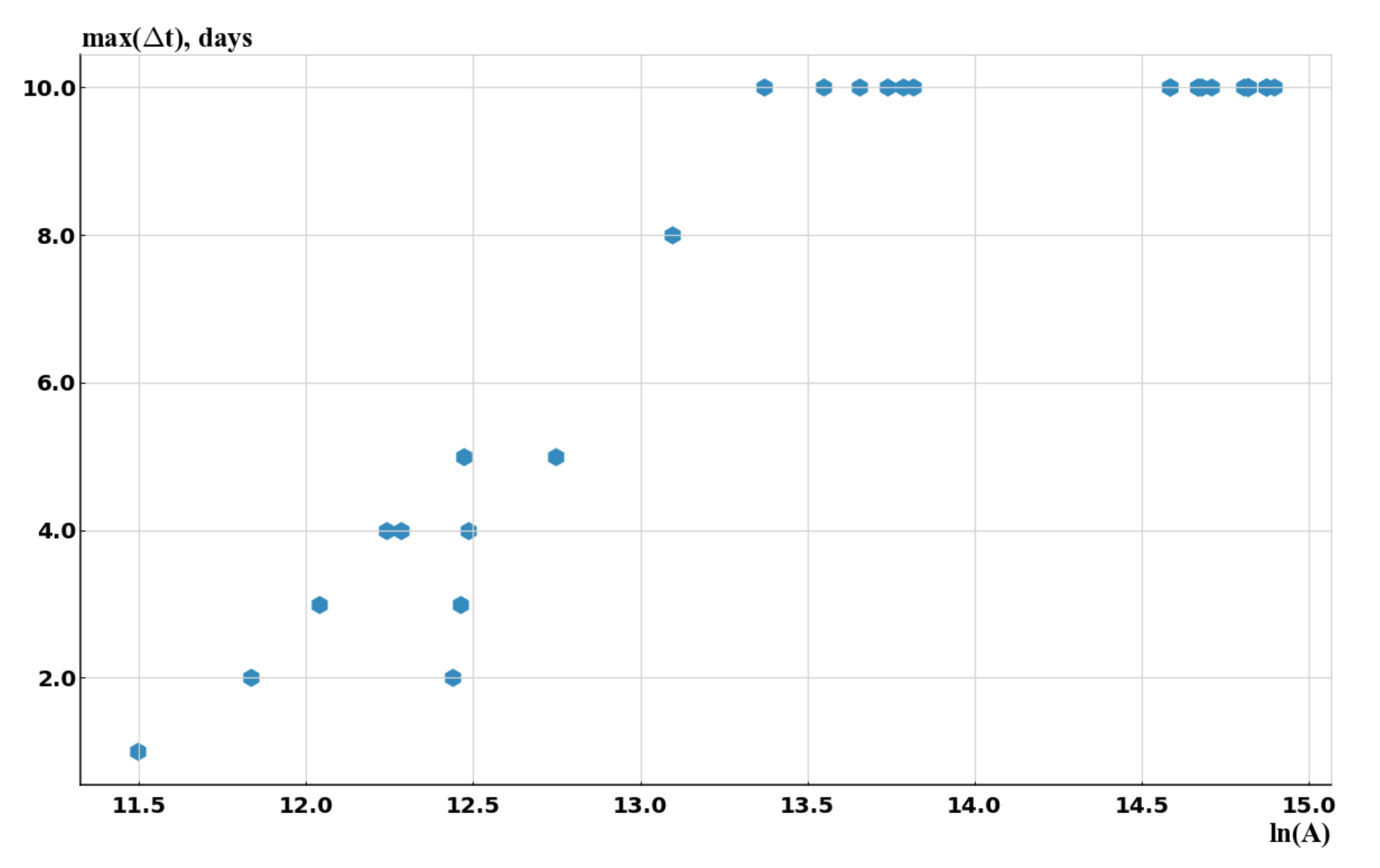
As an example,
Figure 5 shows the relationship between
max(Δ
t) and
ln(A) for the Lower part of the Ob river basin (Region 12 in
Figure 4).
Judging by the point distribution, one can state that, for river catchment areas more than 300,000 km2, forecast efficiency is good for lead times more than 5 days; for areas with 700,000 km2 or more, lead times with good forecast efficiency may reach up to 10 days.
Similar and more detailed relationships for different regions of Russia allows assessing in advance the possibility of using the hydrograph extrapolation method in flow forecasting.
In
Table 4, it is worth noting that application of
f(A, I) =
ln(A) + 1.3
ln(I) as the optimal argument for the Terek river basin (mountainous basin in the south of European Russia) indicates that in this region, the maximum lead time is satisfactory. According to forecasts,
max(∆
t) increases with an increase in the average slope of the river basin surface. This unexpected result has a fairly simple explanation.
The rivers of the Terek basin have the highest values of slopes; the catchments are located mainly high in the mountains. Snow and glacier flow origin predominates here. It provides a smooth shape of the hydrograph in general. The rivers have the smallest slopes, the catchments of which are located mainly on the plain. For them, rain food pre-possesses. It provides the sharp outlines of individual floods and the sawtooth character of the hydrograph as a whole [
20]. Thus, for the Terek river basin, the average slope of the river basin indirectly characterizes the location of the catchment area of the river and its flow origin, and this determines the features of the hydrograph shape and the possibility of its extrapolation.
The hydrograph extrapolation method was used to obtain a forecast of water discharge with a lead-time ∆t from 1 to 10 days. In this regard, the values of the indicator max(∆t), which determines the maximum lead-time of good forecasts, are also limited to 10 days. As a result, for many regions, the relationship of this indicator with the morphometric characteristics f(A, I) becomes nonlinear as it increases and the value of max(∆t) approaches 10. This leads to the fact that the correlation coefficient r, which characterizes the tightness of the statistical relationship and the degree of its linearity, underestimates the actual tightness of the relationship between max(∆t) and the argument f(A, I). If discharges are predicted with a lead time of more than 10 days, the nature of this dependence would be linear in the entire range of values and the correlation coefficients r would be greater.
For all selected regions, the relationship of the max(∆t) and morphometric characteristics f(A, I) turned out to be insufficiently close to allow determination of the maximum lead time of satisfactory forecasts at certain values of area A and the average slope I of a catchment. However, these relationships allow estimation of the extremely low value of f(A, I), which provides satisfactory forecasts with a sufficiently long lead time, and an extremely high value, in which satisfactory forecasts are possible only with a short lead time or are impossible at all (max(∆t) = 0).
Thus, identified regional dependencies allow estimating the threshold values of the area and average slope of the catchment, beyond which, satisfactory forecasts are possible with a sufficiently long lead time, or, conversely, only with a short lead time or are not possible at all.


