1. Introduction
Contemporary and future challenges in socially responsible portfolio management consider a wide range of important issues including both ethical investing and performance analysis, as well as sustainable investment strategies. Authors find interesting various important works in the area of the research [
1,
2,
3]. Conventionally, the stock market is known for providing investors with investment to place their surplus funds [
4,
5,
6,
7] while providing companies with the opportunity to raise a variety of capital and expand their business [
8]. On the other hand, while this performance has made the financial market one of the mainstays of economic research and digitalization, anecdotal evidence over the past two decades has emphasized the trading of commodities in the cash and derivatives markets as an alternative investment class for traditional securities [
9,
10,
11]. Therefore, from a policy perspective, understanding the drivers and consequences of volatility in each market is important for formulating policies that ensure macroeconomic and macroeconomic stability [
12] and sustainability, which leads to the appropriate selection of investment portfolios [
13,
14,
15]. For investors and consumers, on the other hand, this knowledge helps them to predict prices, diversify risks, and develop strategies for hedging, trading derivatives, and securities optimization [
12].
Accordingly, there is currently a vast body of literature examining how macroeconomics affects the performance of financial markets and commodities to achieve sustained positive impact in overall economy. Importantly, as an empirical representative of macroeconomic conditions, studies in this literature often use one or more different time series indicators such as unemployment rate, industrial production, GDP growth, and inflation. These variables are only available with a monthly or quarterly average with a significant delay and, therefore, hide a lot of information [
16].
The researchers consider financial markets and the volatility index (VIX) from a specific point of view regarding the economic indicators based on deep learning algorithms and the sustainability concept. The authors take into account that if the value of the VIX increases, the S&P 500 is likely to fall, and if the value of the VIX implicit volatility index decreases, the S&P 500 is likely to be stable. This creates uncertainty and insufficient accuracy, so it is necessary to provide a model for a near-optimal state. The purpose of the research consists in development of an approach allowing the use of deep probabilistic convolutional neural networks based on conditional variance as a linear function of errors with the aim of estimating and predicting the volatility index (VIX). From the authors’ point of view, the developed approach could extend the implementation of the sustainable portfolio management methodologies.
2. Literature Review
In the field of estimating and predicting fluctuations in stock exchanges and financial markets, many studies have been conducted, the most recent of which is a case study. In [
17], stock exchange data are analyzed using fuzzy clustering methods for clustering data, but since this method has weaknesses in training, artificial neural networks have been used to improve clustering. The authors of [
18] present a graph-based approach to forecasting stocks using big data. First, the dynamic time warping algorithm is used to find a similar pattern between the data and their adjacent data. In the following, a stepwise regression analysis has been used to extract the features. In another study presented in [
19], stock market predictions were made using an artificial neural network. NASDAQ shares are the subject of this study, which is forecast to be conducted in the period from 28 January 2015 to 18 June 2015. The use of the particle swarm optimization (PSO) algorithm with a neural network with fuzzy functions to predict the stock market of Mexico based on statistical arbitrage is presented in [
20]. The use of the first and second fuzzy types along with the neural network for classification and the PSO algorithm for extracting features from stock market data is considered. The presentation of a classification method is conducted with an observer and with the strengthening of input and training in [
21], which uses a standard data set called KOSPI based on statistical arbitrage.
Reference [
22] presented the role of the US implicit volatility index in predicting fluctuations in the Chinese stock market by examining evidence of heterogeneous autoregressive (HAR) models. The purpose of this article is to evaluate the role of this proxy in predicting fluctuations in the Chinese stock market. To this end, the authors of this study have developed six HAR models to change the implicit volatility index to predict fluctuations in the Chinese stock market. In-sample and out-of-sample results show that changes in the tacit volatility index can improve the forecast of fluctuations in the Chinese stock market, but mainly show the improvement for predicting bad fluctuations instead of good fluctuations. In addition, such a forecast improvement is measurable in the short-term forecast horizon, but weakens as the forecast horizon increases. The study in [
23] examines whether China’s volatility index can reflect investor sentiment. This study examines whether China’s official volatility index can indicate investor interest. Short-term, medium-term, and long-term fluctuations are obtained by EEMD. Experimental results show that all components of the implicit volatility index can reflect investor sentiment at the relevant level. The findings of this study confirm that the tacit volatility index can reflect the common feelings and expectations of Chinese investors at different time scales.
3. Materials and Methods
Theoretically, various channels have been supported in the literature to support the relationship between macroeconomic conditions and stock market volatility [
24,
25,
26,
27,
28]. Some researchers argue that this relationship is attractive given the potential of macroeconomic conditions to influence corporate cash flows and systematic overall risk [
29]. The two main approaches to measuring stock returns, such as dividend mitigation model and arbitrage pricing theory, provide an important theoretical framework for the relationship between macroeconomic conditions and stock prices. For example, as an absolute pricing model, the dividend discount model predicts that any (unforeseen) entry of new information about real economic activity will drive stock prices/returns through the impact on dividends [
30]. On the other hand, as a relative pricing model, arbitrage pricing theory predicts the expected return on investment based on its risk, which is measured by the sensitivity of individual assets to the market return index.
Many investors are familiar with the VIX or volatility index, which measures how much investors expect to see the S&P 500 fluctuate. Economic VIX is important now because its history during the decades after World War II shows that stocks perform best when economic volatility in the United States are at their lowest or highest. VIX is a rate at which the price of a security increases or decreases for a particular set of returns. Volatility is measured by calculating the standard deviation of annual returns over a specified period of time, indicating that the price of a security may increase or decrease and measures the fluctuations of a security risk. It is used in the option pricing formula. Volatility reflects the pricing behavior of securities and help to estimate volatility that may occur in the short term. Over the next year, due to the COVID-19 pandemic, we will have an economic volatility that has not been seen before in the post-war period [
31].
The volatility index is released every 15 s from 2:15 am to 8:15 am and from 8:30 am to 3:15 pm. The final settlement value for futures and VIX options is calculated based on the Special Opening Quotation (SOQ) of the volatility index using the open prices of the weekly SPX and SPX options that expire 30 days after the expiration date of the VIX. The initial prices of the SPX options used in SOQ are set by an automated auction mechanism in Chicago Board Options Exchange (CBOE) options that matches locked or reverse buy orders and quotes in the e-order book when opening trades. Even if the SPXW options expire at 3:00 pm, the settlement amount is calculated at the same time as the SPX options (8.30 am). The CBOE uses Equation (1) to calculate the VIX [
32]:
where
T is the expiration time (US risk-free interest rate). Treasury performance curve for expiration date of the relevant SPX options includes
F, the forward price of the S&P 500, and
, which are the first strikes below the level of the
F and
of the strike price of the
i-th
option.
is the midpoint of the bid price of the option with the strike
.
More precisely,
T is defined as in Equation (2) [
32]:
where
shows the remaining minutes until current midnight, and
indicates minutes from midnight to 8:30 am for standard SPX options and a few minutes from midnight to 3:00 pm. For SPXW expiration, the
variable is the total number of minutes between the days between the current day and the options expiration day.
F is defined as in Equation (3) [
32]:
It should be noted that all VIX calculations are calculated for short-term and subsequent options. The CBOE identifies short-term options with a remaining time of 23 to 30 days and subsequent options with a remaining time of 31 to 37 days. If two consecutive zero bids occur, not all of the less objectionable options will not be considered. Considering these rules and parameters,
and
can be calculated, which are the short-term and subsequent components of the VIX. It takes an average of 30 weighted days of
and
to obtain the value of the VIX (Equation (4)):
where the variables are as follows:
: Expiration time (as a fraction of the total number of minutes per year) of short-term options;
: Expiration time (as a fraction of the total number of minutes per year) of next period options;
: Number of minutes to settle short-term options;
: Number of minutes to clear the next period options;
: Number of minutes in 30 days (43, 200);
: Number of minutes in a year 365 days (525, 600).
Based on the model in [
32], which has modeled the estimation of implied and normal VIX (Equations (1)–(4)), a new model with a combination of deep convolutional neural network (DCNN) is presented in this section. In general, models based on deep learning according to [
15,
16,
29,
30,
31] are the most widely used econometric models when studying the implied Volatility and VIX. This research uses convolutional-based image processing principles to predict the VIX and compare it with deep learning models. In the first step, the return to the effects is decomposed according to Equation (5):
where
is the median of
, and
is the error. In this study, it is assumed that
originates from Equation (6):
where
. Hence,
is the conditional variance at time
. Then, the conditional variance of a linear function of its errors and delays is assumed to be (Equation (7)):
In addition to the convolutional deep learning model presented below, a simple method for predicting the VIX is developed. Similar to [
10], who uses historical statistics as a predicted risk, this study calculates the standard deviation of the return series in an
n-day trading window and uses it as a forecast for fluctuations for the next trading day. This is a simple but intuitive method and can be used as a benchmark for evaluating other methods. The parameter to be estimated is only the window length
n. An optimization method similar to econometric models is used to obtain the estimate, meaning that the best window length is a value that can maximize the probability of sample data to perform image recognition. Vector formulas can be used to describe the DCNN as in Equation (8):
where
is the hidden state at time
t, and
represents the input at time
t. σ is the activation function.
This research uses LeakyReLU for the convolutional neural network. is for the torsion layer (convolution), and is for the polling layer (random and maximal). Similarly, is for the fully connected layer, which gives the final result to the output layer. shows point multiplication.
As discussed at the outset, a probability-based loss function is used when training deep neural network models in estimating the VIX. If
is the recurrence series observed from time 1 to time
T,
and
T are the volatilities that the model predicts at the same time step, assuming a normal distribution. The probability of the sample can be calculated as in Equation (9):
Based on this, the log-likelihood function can be obtained according to Equation (10):
Login performance should be maximized through optimization, while deep learning models are always trained by minimizing their loss performance. Therefore, the negative logging possibility should be used so that the performance of the loss is deep in the learning models. To further reduce the computational cost of deep learning models, a simple function is used as the convolutional loss model function as Equation (11):
Once all the models discussed so far have been tested, Equation (11) is used to calculate the probability function of logging the test sample and comparing the values. It does not matter if all the methods are in the training stages or in the experimental stages, the forecasting method is implemented day by day. This means that it predicts volatility in a rolling window, and the window moves forward one trading day at a time. When the day-to-day volatilities are predicted and the
volatility series from time 1 to time
T is obtained, it can be used to calculate Equations (10) and (11) in various processes. Other configuration neural network model settings should also be considered. The number of input layer units is set to 10, meaning that a 10-day recurrence series is used each time. The number of hidden layers is two. The first hidden layer has 40 units, and the second hidden layer has 80 units. The hidden layer activation function is selected as LeakyReLU, and the threshold in these two layers is set to 0.3. The output layer activation function is set to sigmoid. The back-propagation error network is used as an optimizer to train the model. The set size is set to 2048. If the lost portfolio performance is not revoked, there is an early pause. The convolutional neural network model finally combines time with a fully connected layer. If the loss function is a distance function used by other research studies, the linear activation function can be good enough. However, when the probability loss function is used as in Equations (3)–(7), some activation functions, such as the linear function, cannot help the models converge during training. The performance of the LeakyReLU and sigmoid activation function is a good option in the output layer, and the proposed model can be successfully trained [
33,
34,
35].
4. Empirical Results
The available data for predicting the implied VIX have six characteristics, namely Volume (value of VIX), Date (related dates), VIX Open (the part of VIX that is open to buy), VIX High (upper rates of implied VIX), VIX Low (lower rates of implied VIX), and VIX Close (the part where closed to buy VIX). These are the data characteristics and the data volume is 7898. The data are normalized and there is no need for a normalizing step. When training deep neural network models in predicting VIX, a probability-based loss function in DCNN with layering settings and the LeakyReLU stimulus function model and other settings, mentioned in
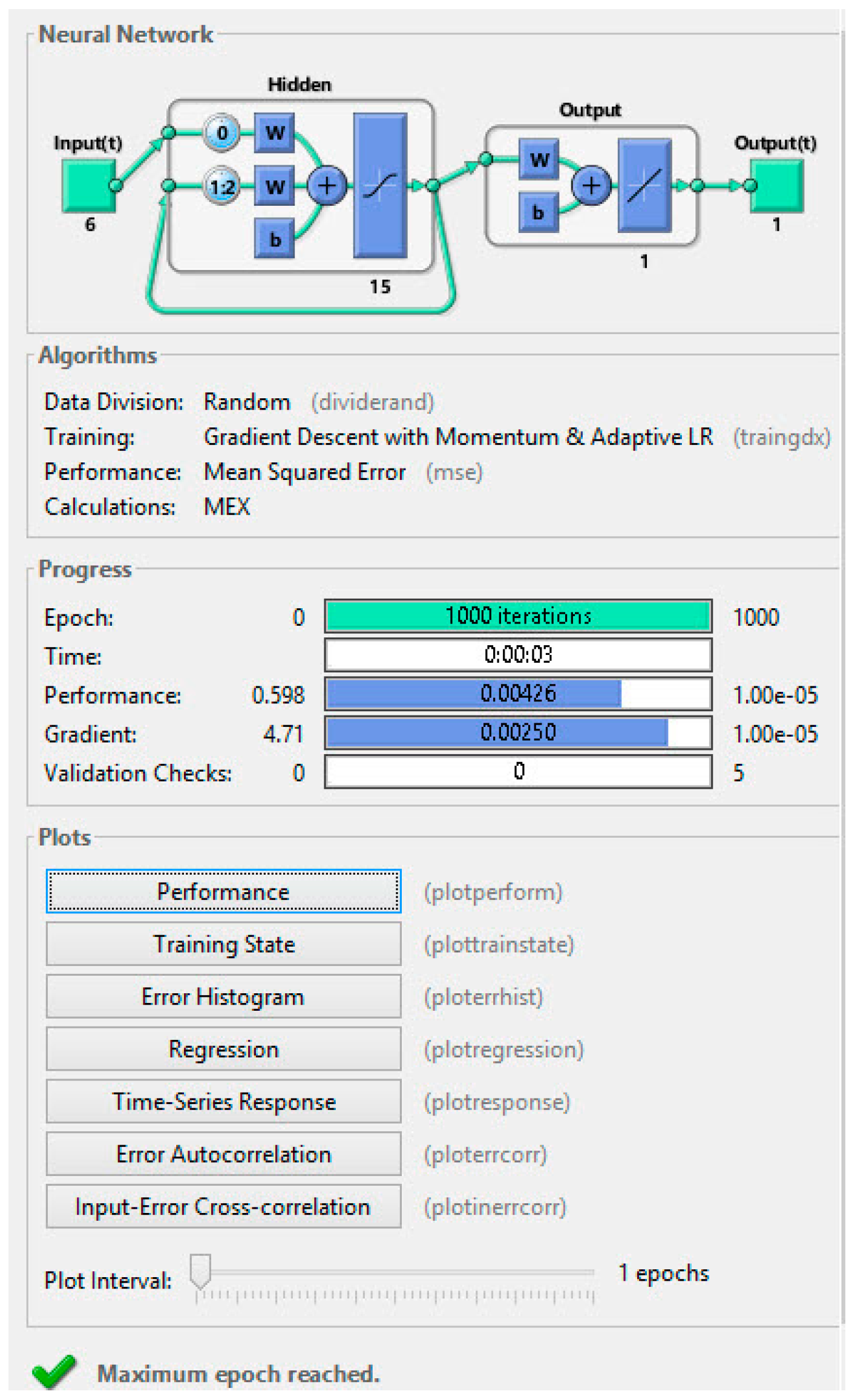
Section 3, are used. The data are transmitted to a DCNN. It should be noted that the DCNN operates as a deep multi-channel network during the prediction operation due to its probabilistic state. Therefore, the structural representation of this neural network is essential, and adjusting its parameters is very important. Therefore, after training and testing, the data according to the approach presented in
Section 3,
Figure 1 illustrate the general neural network structure after training and testing the data. At the end, the image recognition mode with probabilistic DCNN is used based on conditional variance as a linear function of errors to improve the prediction of the network results and showing the VIX time series.
In this structure in general, once the DCNN makes this prediction, and since the results are not satisfying, the conditional variance method as a linear function of the errors also improves the results as much as possible and reduces the dimensions so that a more accurate forecast can be made for a certain period of time. The data sharing method is considered random. The core of training for DCNN is the use of the descending gradient method with momentum and adaptive training rate. In addition, to evaluate the efficiency of DCNN, the mean square error function has been used. The number of repetitions for data training is also a maximum of 1000.
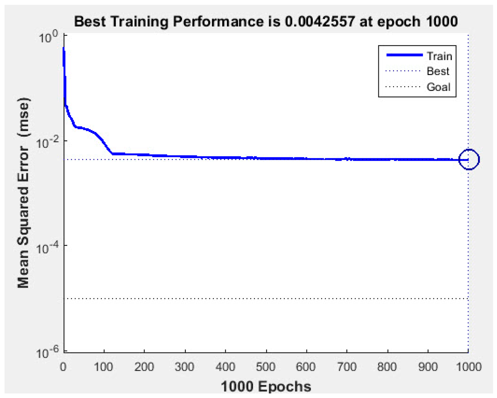
Figure 2 shows the performance of a DCNN. Accordingly, at approximately 200 repetitions, the method converges and the data training diagram (blue diagram) reaches the goal function.
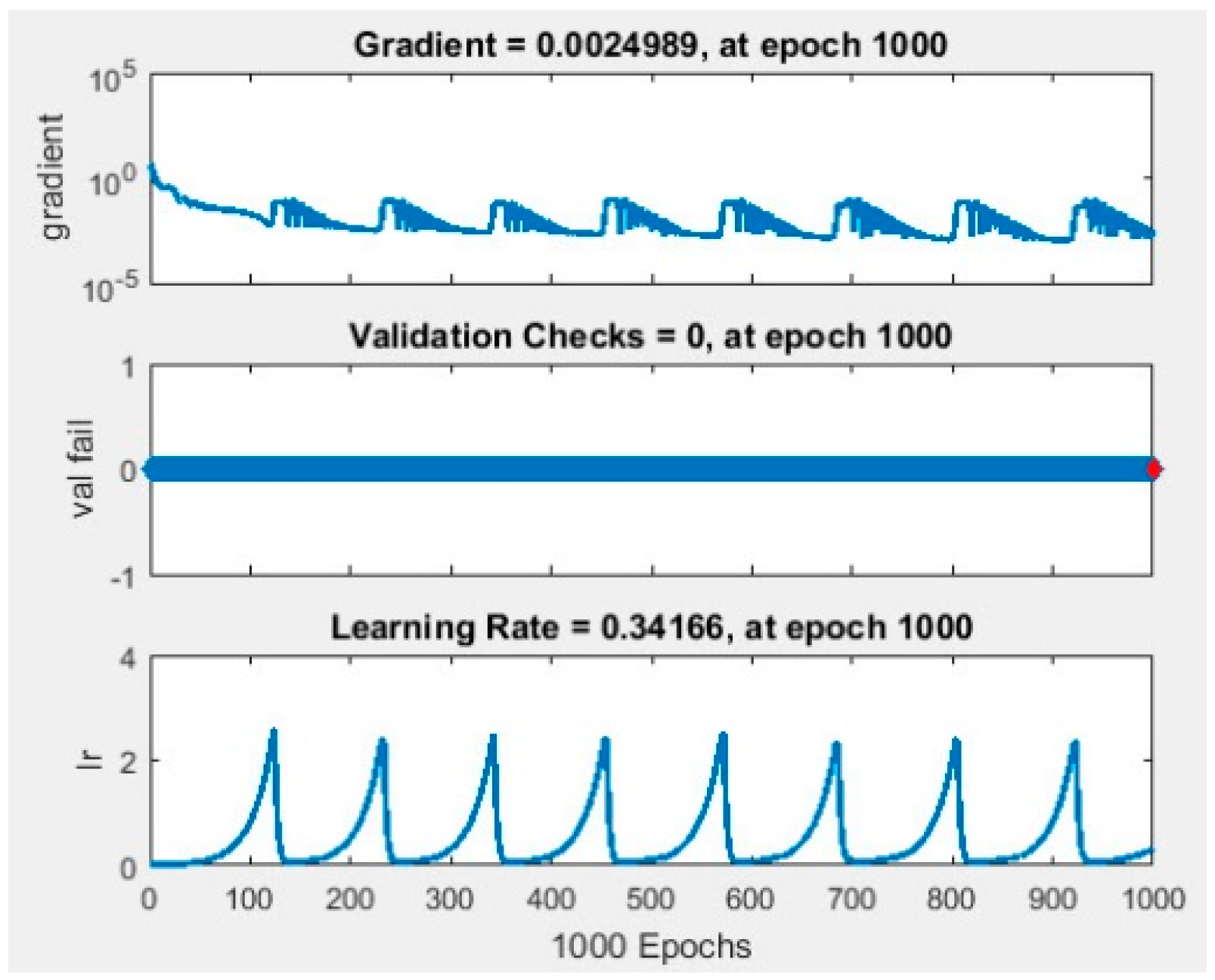
Figure 3 shows the training modes with the gradient, validation, and training rates. In the upper part, the gradient rate during training in 1000 repetitions is equal to 0.0024989; in the middle part, the validation rate of the Kfold method is equal to 0 per 1000 repetitions; and in the lower part, the training rate in 1000 repetitions is equal to 0.34166.
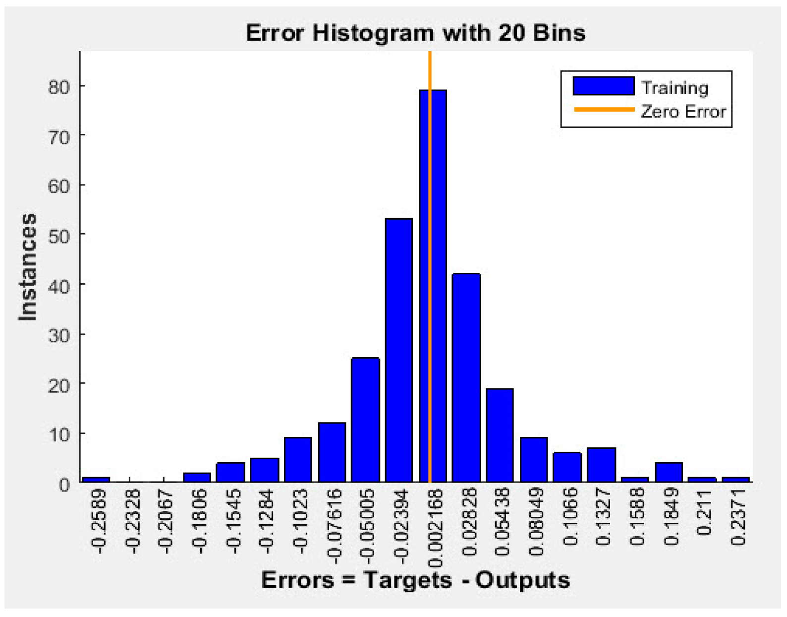
Figure 4 shows the error histogram for the final goals and outputs of prediction performed by the DCNN approach based on conditional variance as a linear function of the errors, most of which are in the training phase.
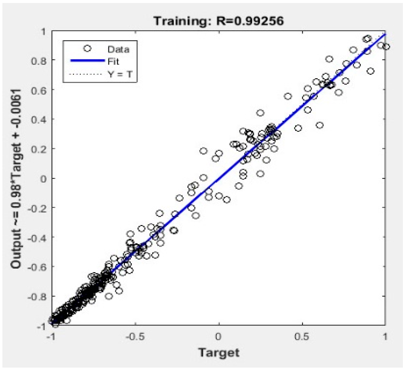
Figure 5, shows that the data are fitted on the regression line as well as the output (goal) as much as possible.
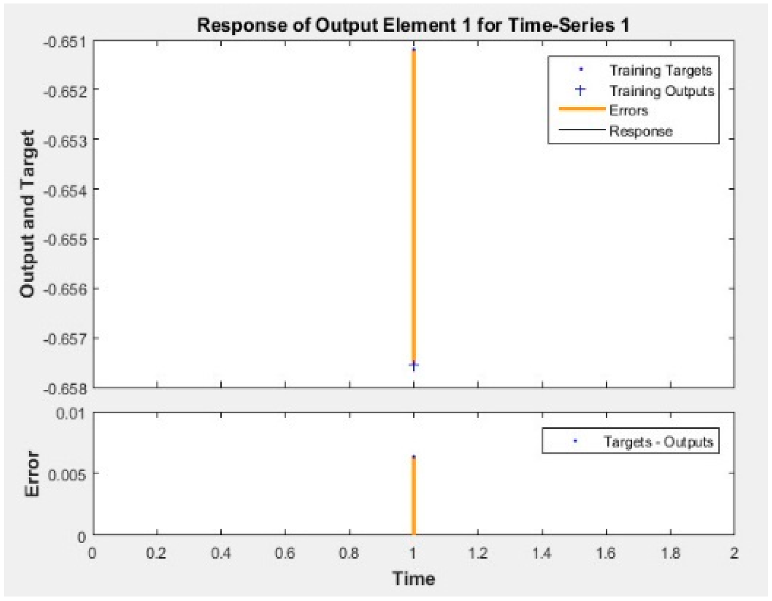
In
Figure 6, at its initial time, there is an error in identifying training objectives and responses, which is then retrained by optimizing the final prediction of the VIX by conditional variance as a linear function of the errors.
Figure 7 shows that there is an autocorrelation error in the DCNN approach, about 0.004%, which is a very small error for this evaluation criterion.
Figure 8 shows that there is no input-error cross-correlation. Moreover, a representation of data prediction with DCNN based on conditional variance as a linear function of errors can be seen in
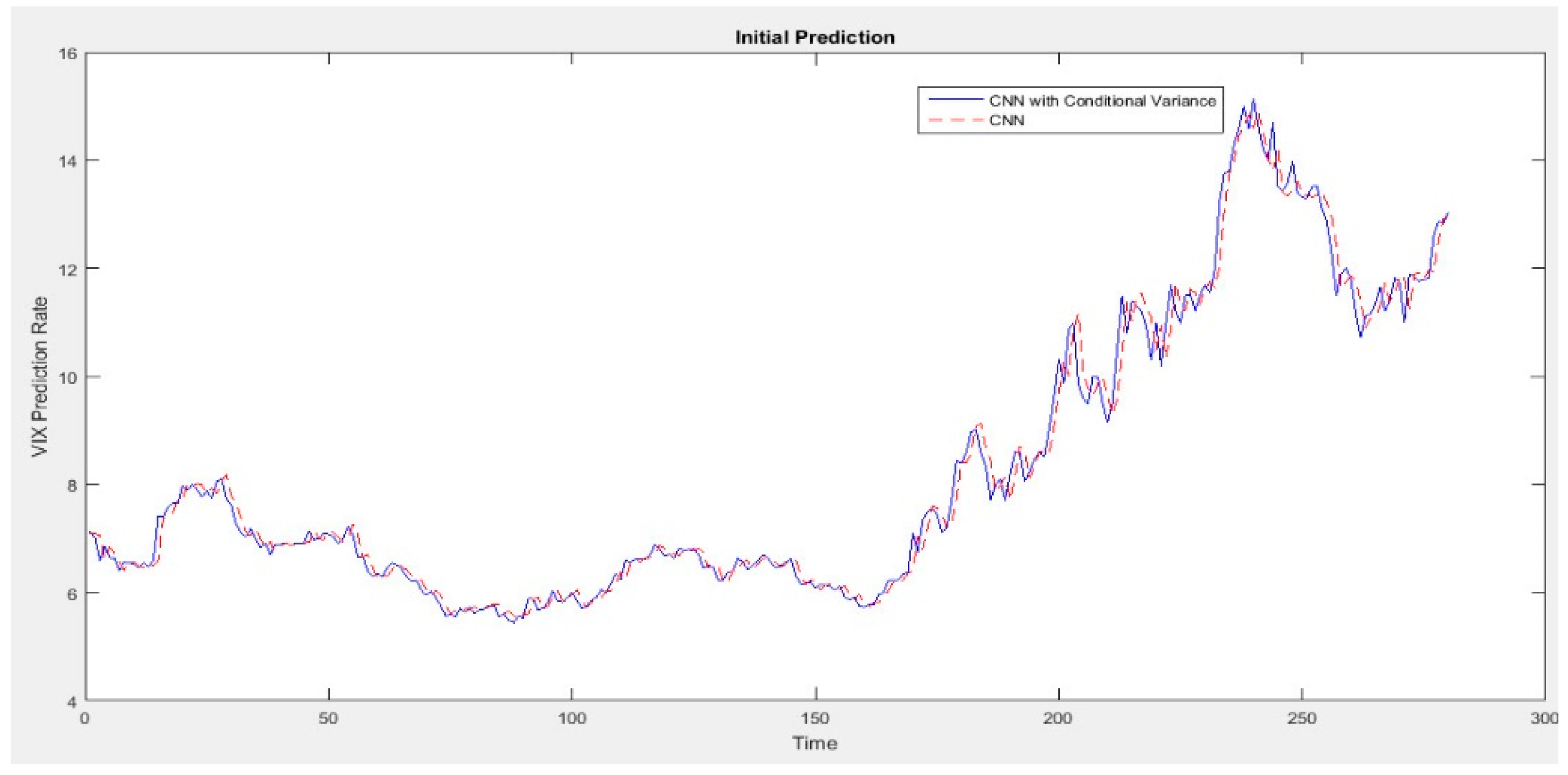
Figure 9. The data are examined for the next 300 days for forecasting. The blue diagram shows the proposed and combined approach of the DCNN based on conditional variance as a linear function of the errors, and the red diagram shows the use of the DCNN alone. It is clear that in all areas, the results of the combined approach are better than using only the DCNN.
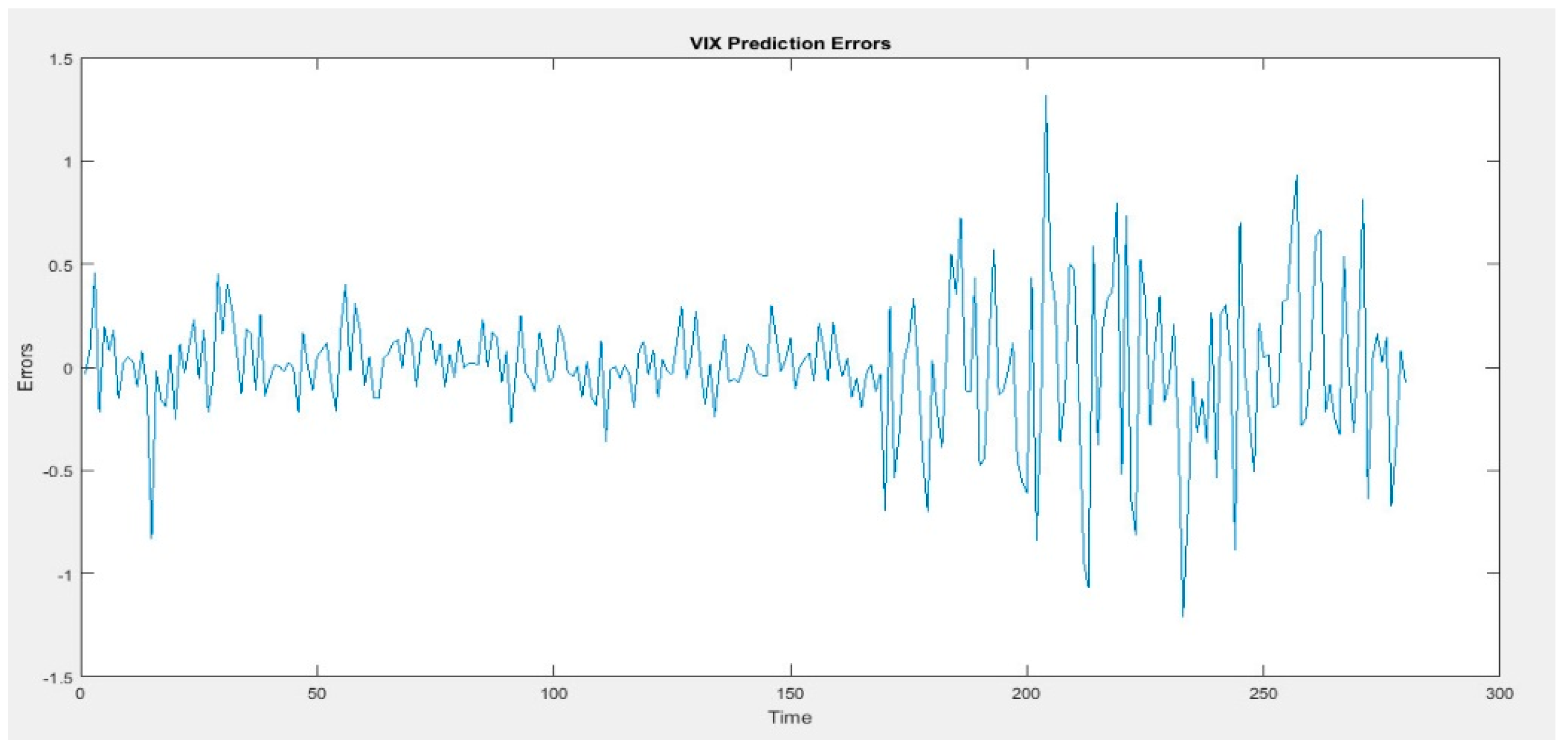
The index of possible errors of the implied VIX of the hybrid approach at the time of prediction is shown in
Figure 10. It is clear that there are errors in the forecast time in 300 days, which is in the range of 0 to 1.4%. it can be concluded that the precision of the proposed approach has an average prediction of up to 98%.
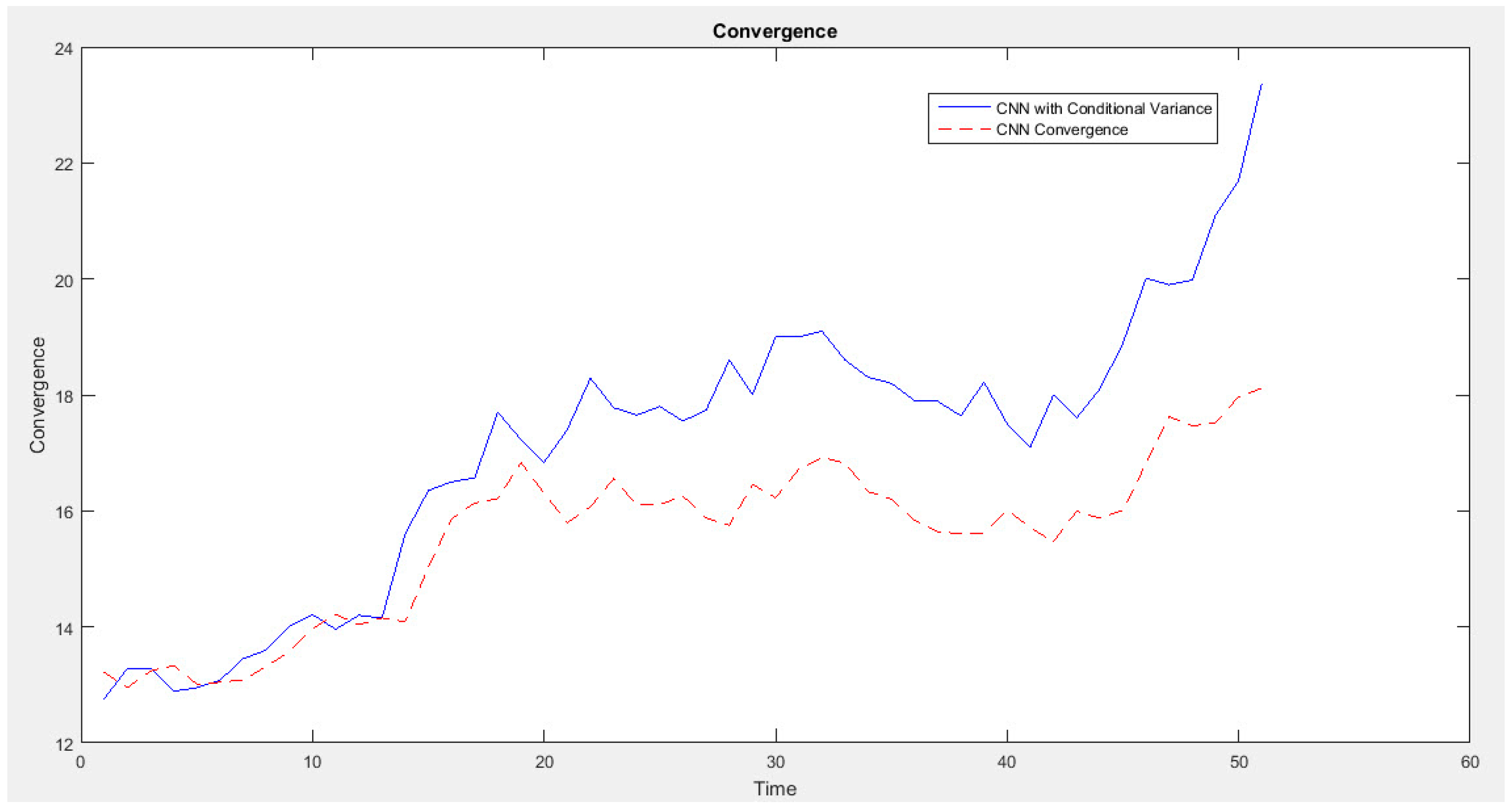
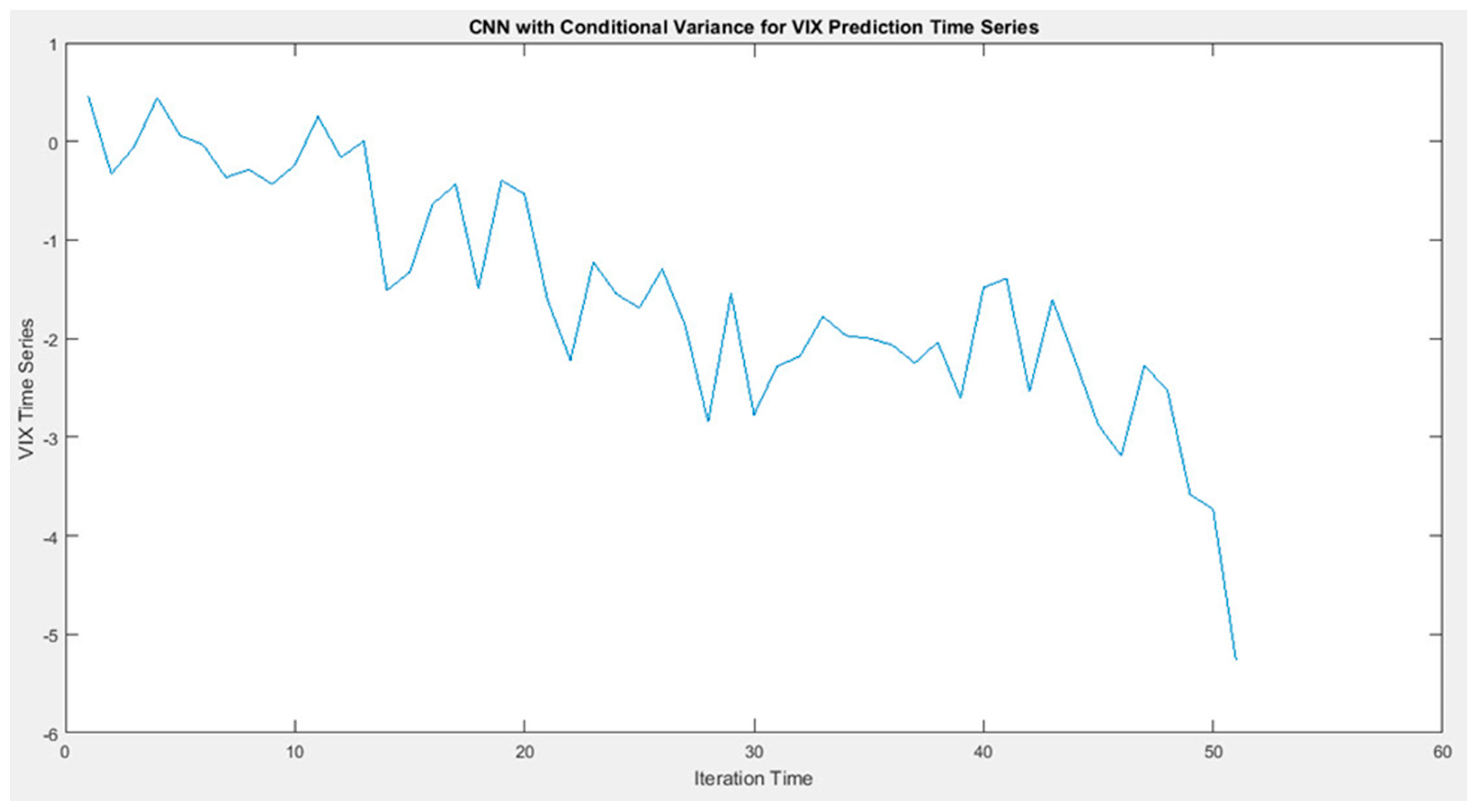
Figure 11 shows that the combined approach of the deep convolutional neural network based on conditional variance as a linear function of errors (blue diagram) has a faster convergence rate than the red diagram using only the deep convolutional neural network. Finally, the time series for the deep convolutional neural network based on conditional variance is plotted as a linear function of the errors, which is shown in
Figure 12. This diagram is declining, which shows an improvement in the proposed approach.
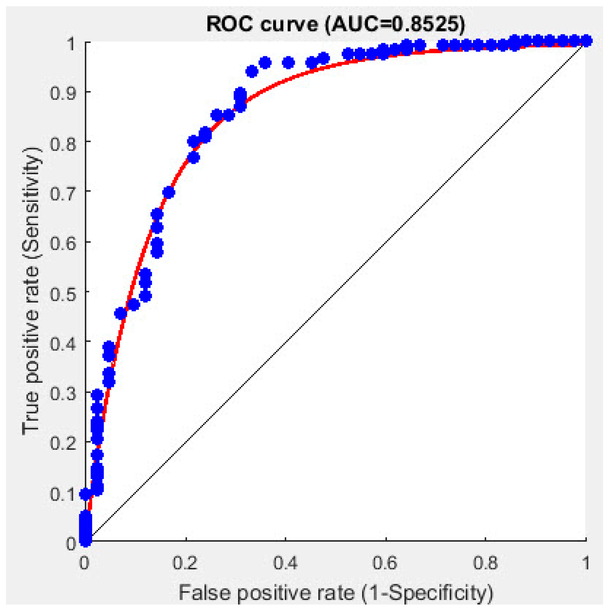
In addition, two other criteria have been used for evaluation, which are the receiver operating characteristic (ROC) curve and the Area Under the Curve (
Figure 13). The ROC curve is red, and the middle line is the regression. The higher the fit of the data on the ROC, the better the AUC. The AUC value is 84.60%, which is a good rate. In general, the results of the evaluation criteria are shown in
Table 1.
5. Conclusions
Since sustainability has become the major trend in every aspect of the academic, financial, and industrial sectors, together with profitability and some other factors, corporate social responsibility is considered as a major concern for investing decision-making process in financial markets and investors tends to invest and select portfolios in socially responsible corporates. Authors tried to make a contribution to the theory of socially responsible portfolio management. The developed approach allows potential investments to make decisions regarding so important topics as ethical investing, performance analysis, as well as sustainable investment strategies.
The implied volatility index (VIX) is a technical index and a security index that can include all trades in one transaction. The VIX is arguably the best measure of risk measurement available to investors and can be used effectively by any trader in any market. This research identifies what VIX is and how it works. The implied VIX is a measure of traders’ expectations for volatility in the S&P 500. It is like a chart, and the higher it goes, the higher traders’ expectations of short-term market volatility are. Based on the proposed model, the use of deep convolutional neural network (DCNN)-based on conditional variance as a linear function of errors was presented with the aim of predicting the implied VIX performed by a valid data set considering its six characteristics. The results show that the estimation of the implied VIX for the CBOE volatility index, and the S&P 500 index options are considered, indicating an improvement in precision and evaluation criteria. It has also been observed that the proposed approach, i.e., hybrid DCNN for implied VIX has a more practical range and better results than using only DCNN.
Authors could discuss the implication of the proposed approach taking into account the digital transformation as an instrument for implication of both sustainable portfolio management methodologies and sustainable stock indices, as well as sustainable development goals (SDG). The researchers find different interesting approaches to the implementation of digital twins in logistics [
36] and trade networks [
37] in the context of both socially responsible investments [
38] and individual sustainable investment [
39]. Definitely, authors should take into account calibrating the conditional value-at-risk (CoVaR) of financial institutions based on neural network quantile regression [
40]. In this regard, the use of digital twin and artificial intelligence in a wide scientific area including sustainable information and reporting and predicting the volatility index, and investing could be a topic for future research.


 ,
, 


