
A Large-Eddy Simulation Study of Vertical Axis Wind Turbine Wakes in the Atmospheric Boundary Layer


Abstract
:1. Introduction
2. Large-Eddy Simulation Framework
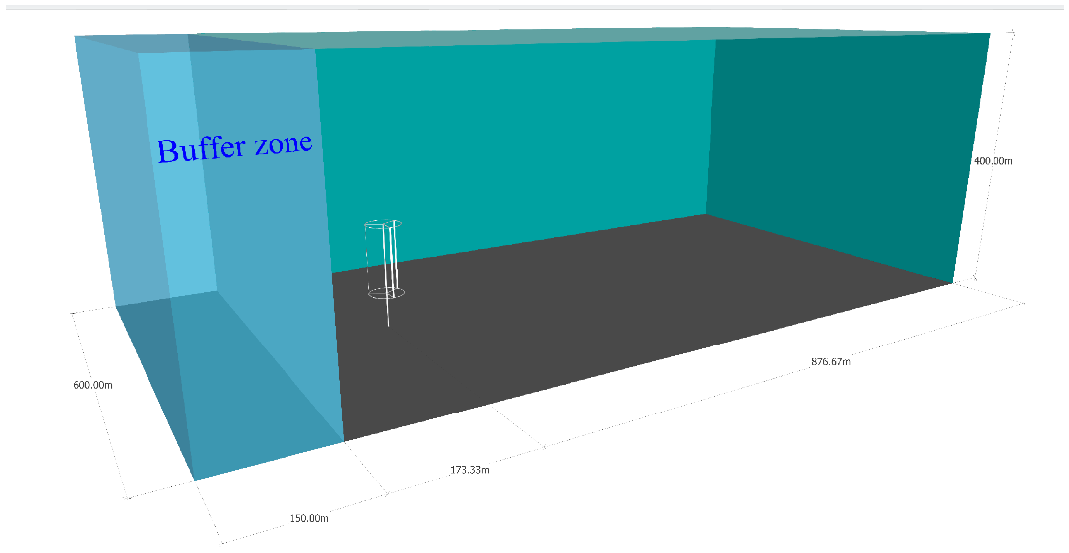
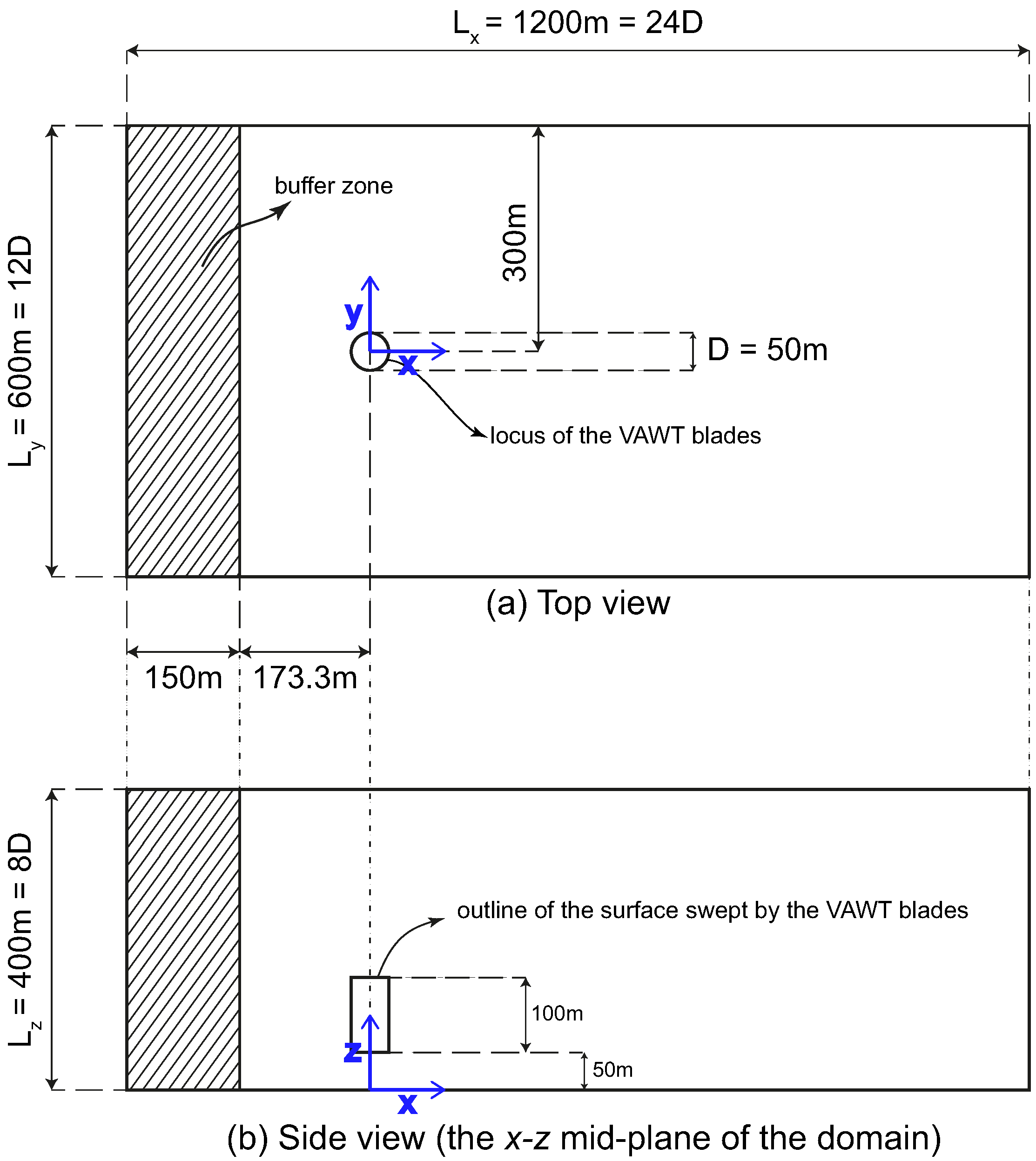
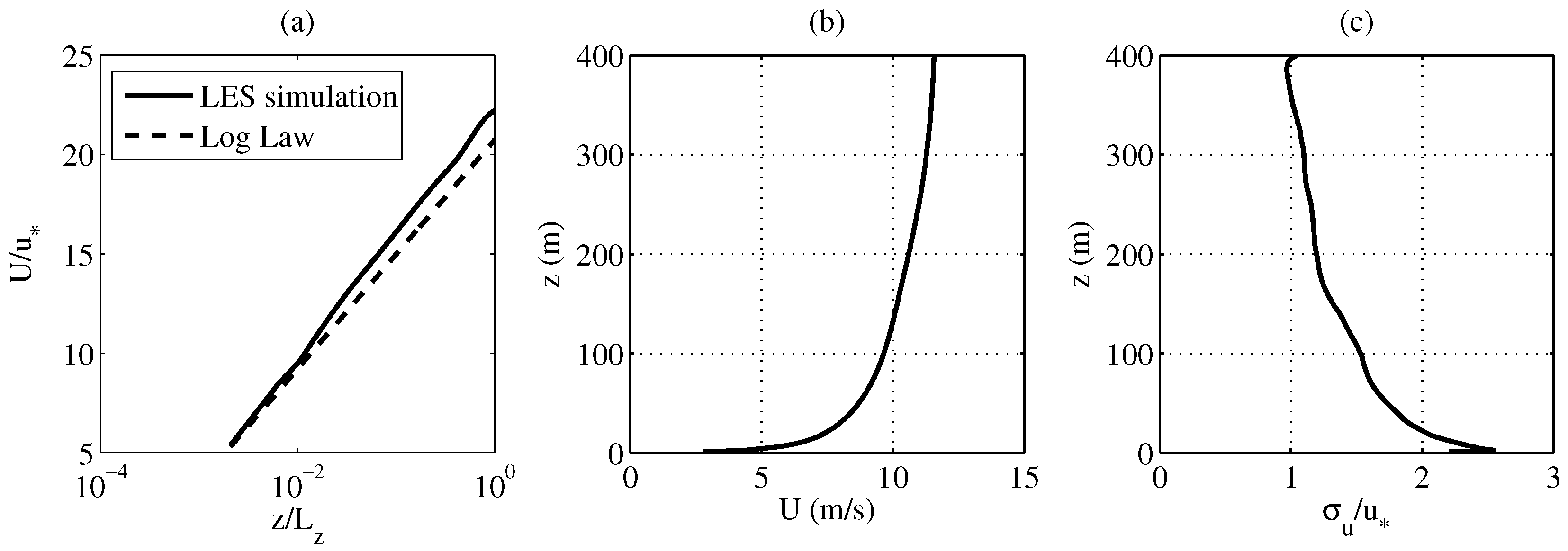
3. Numerical Setup
4. Results and Discussion
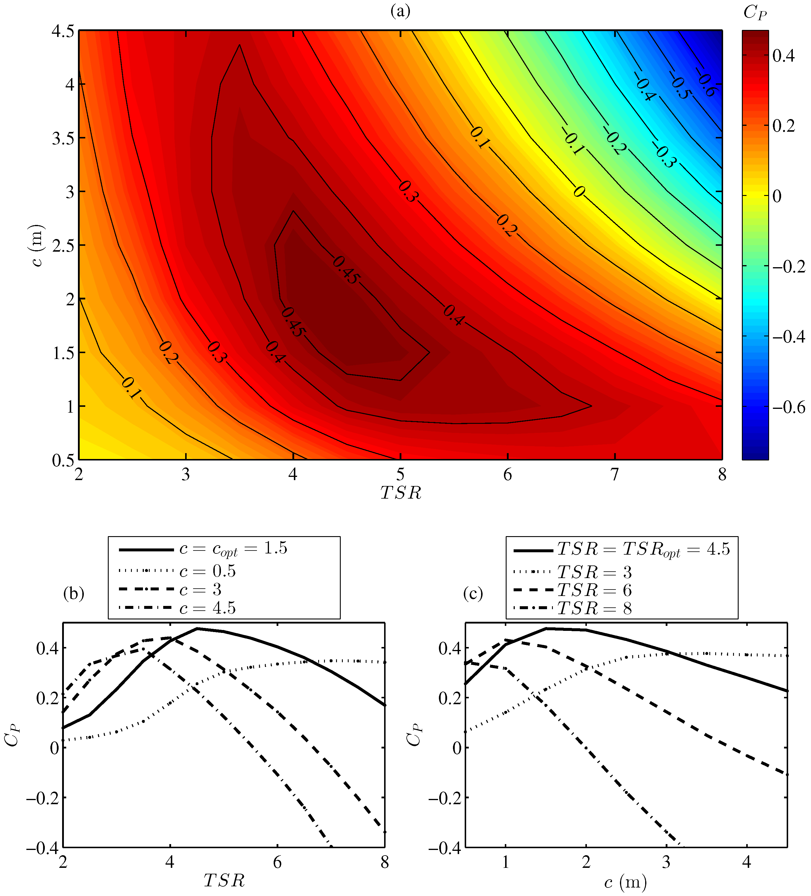
4.1. Turbine Performance and Power Extraction
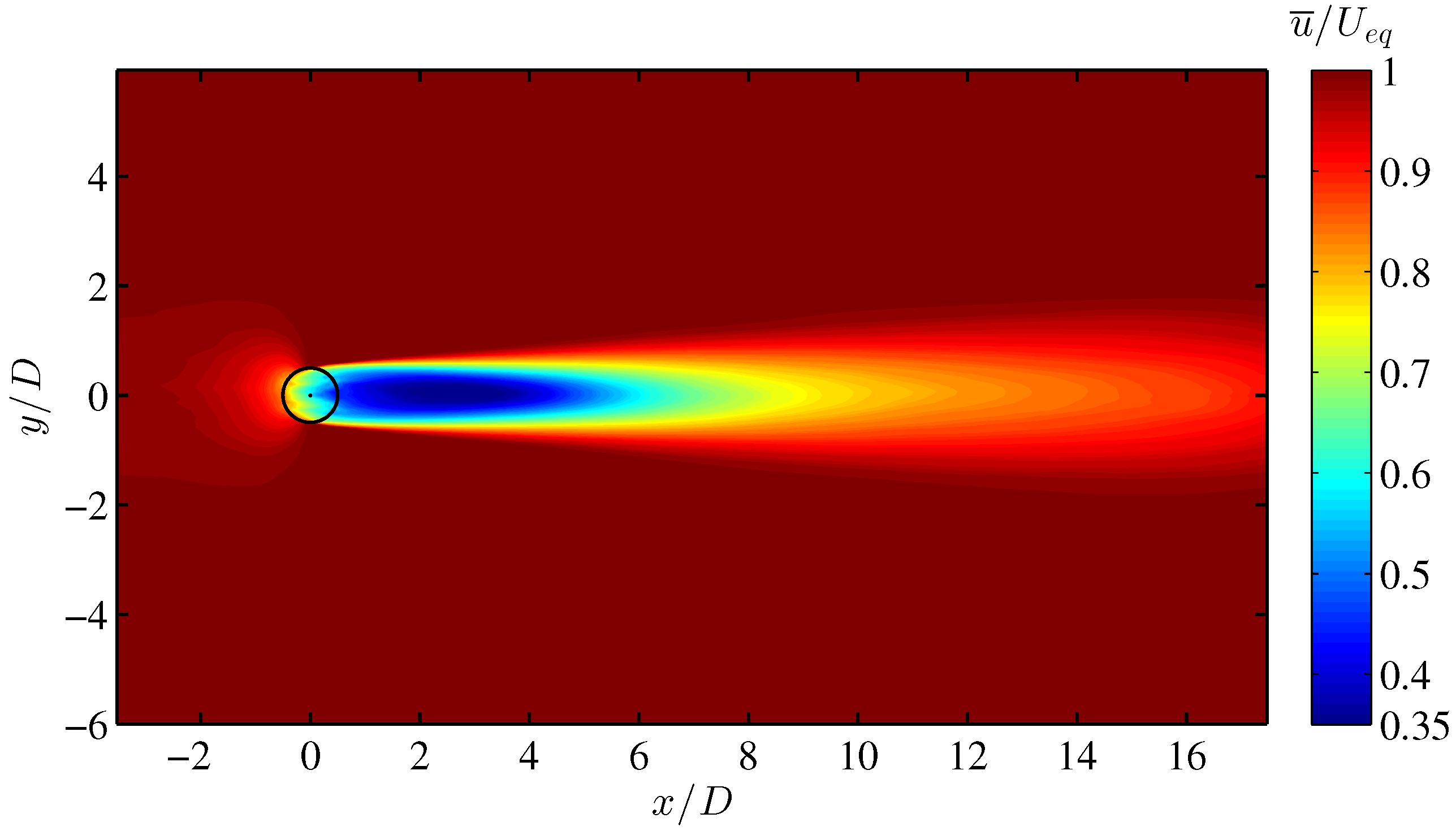
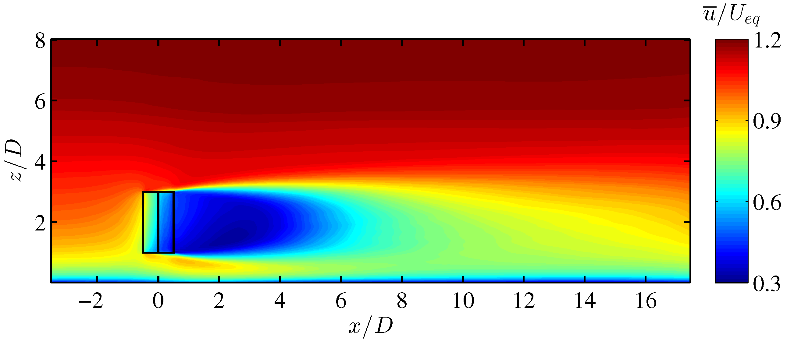
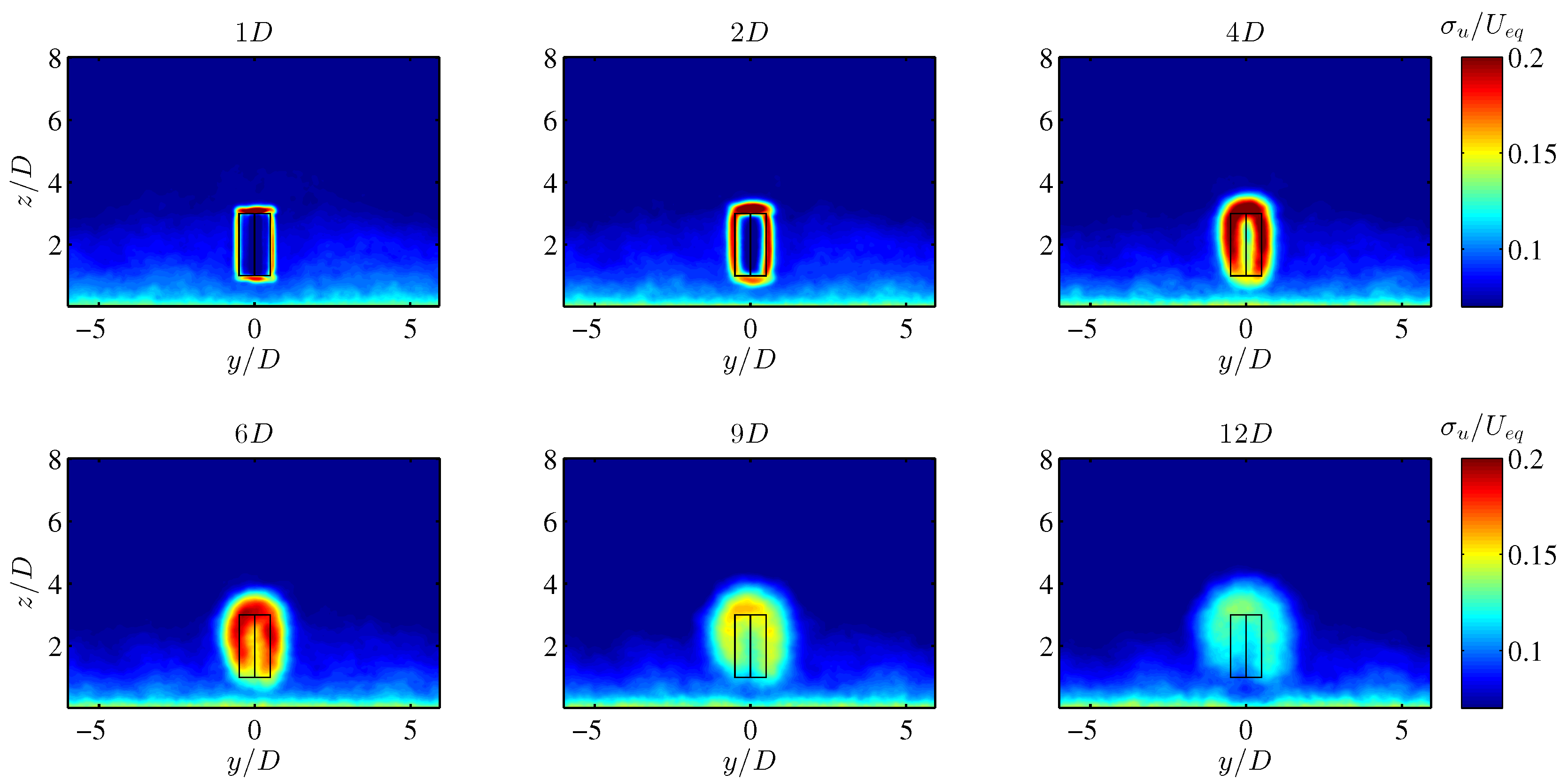
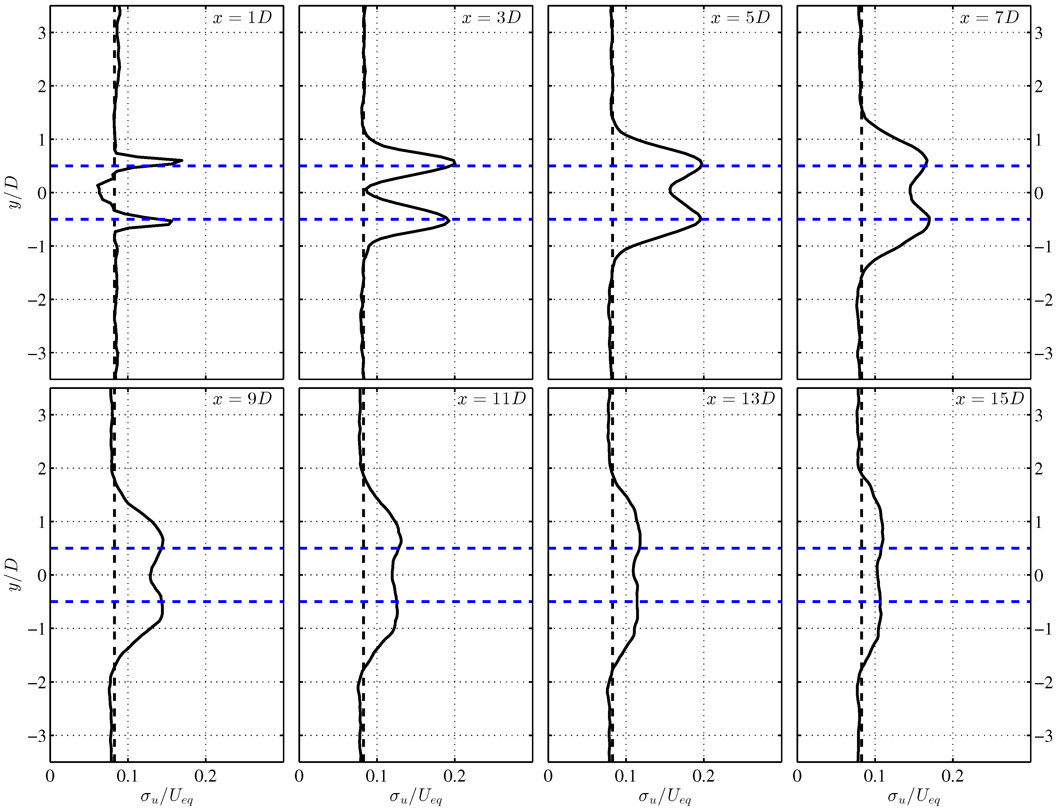
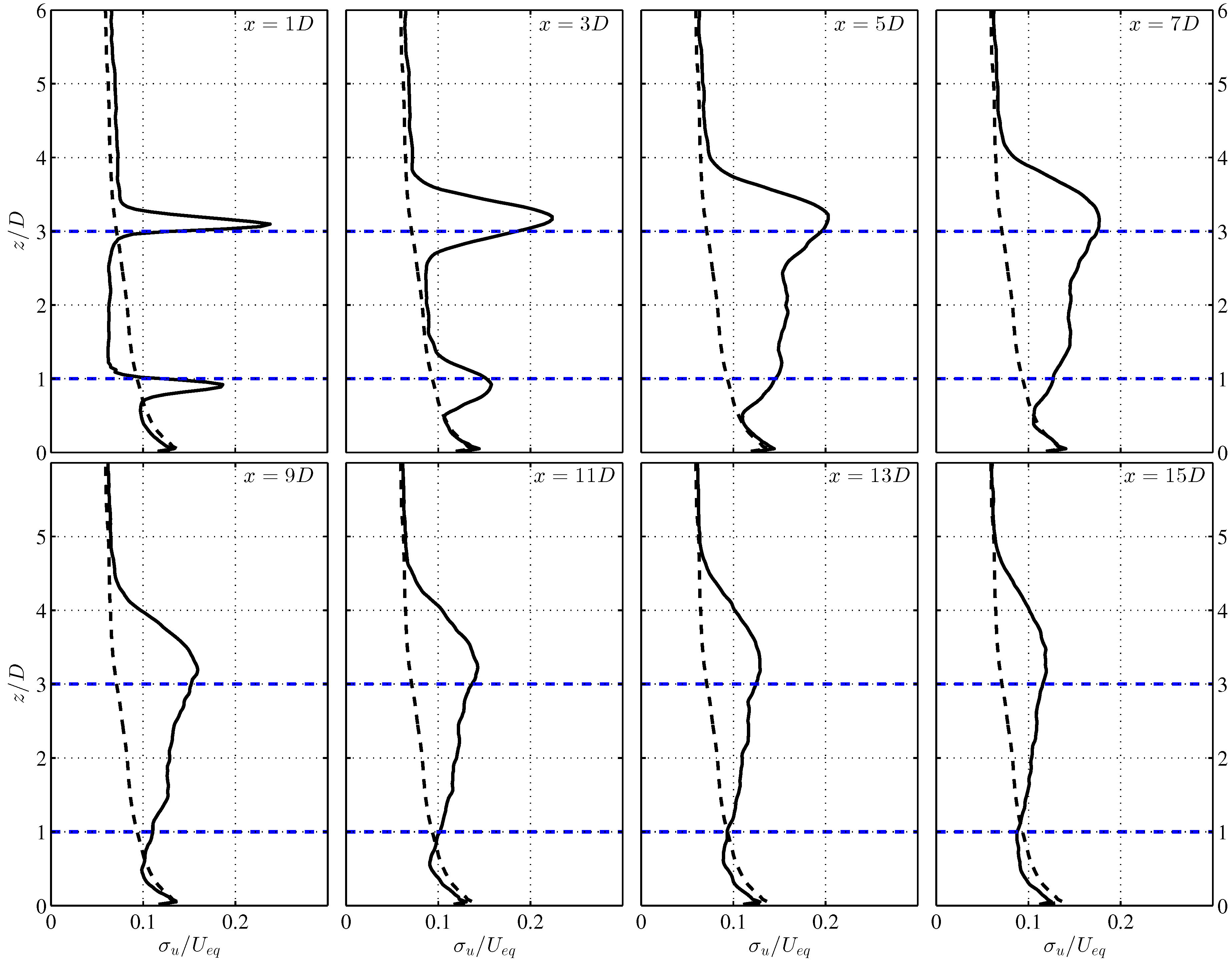
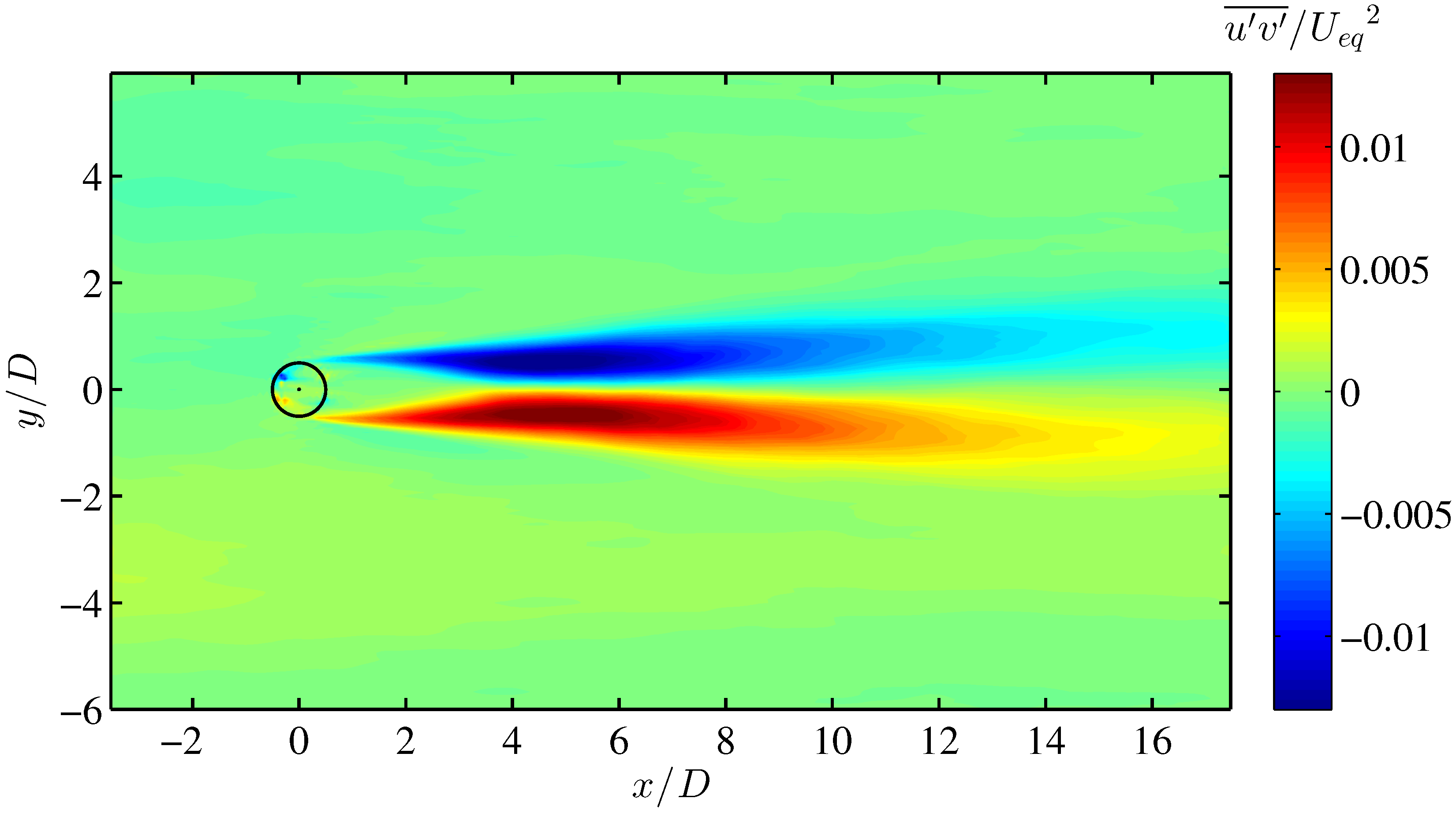
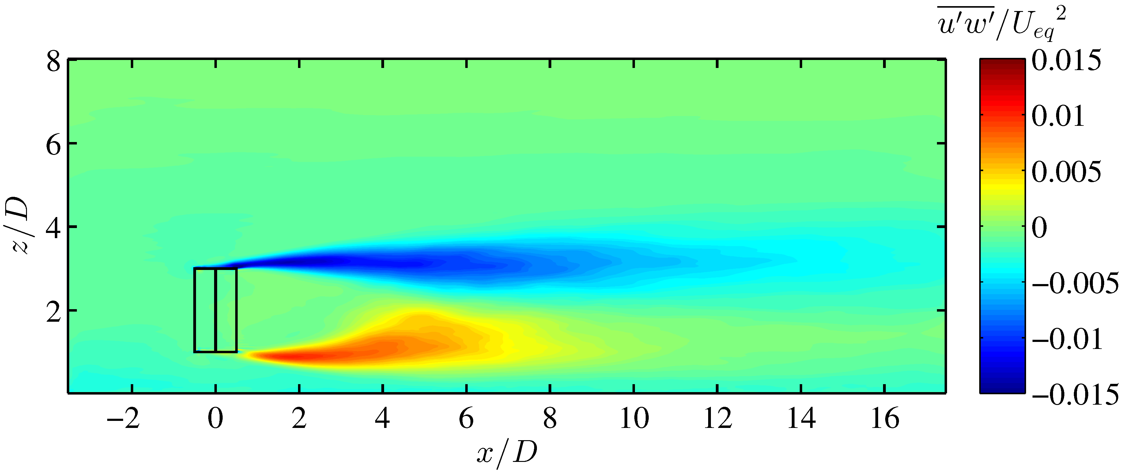
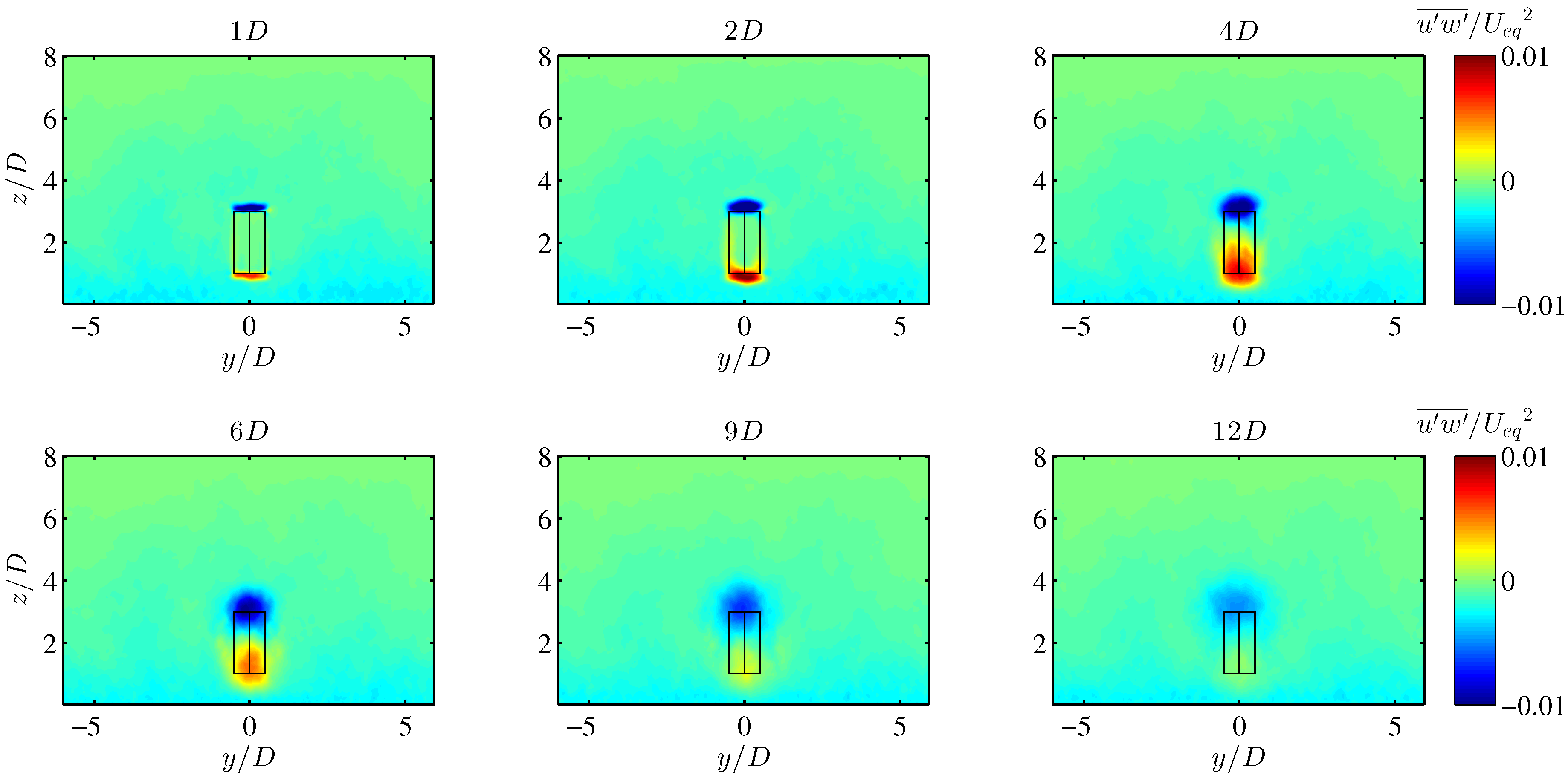
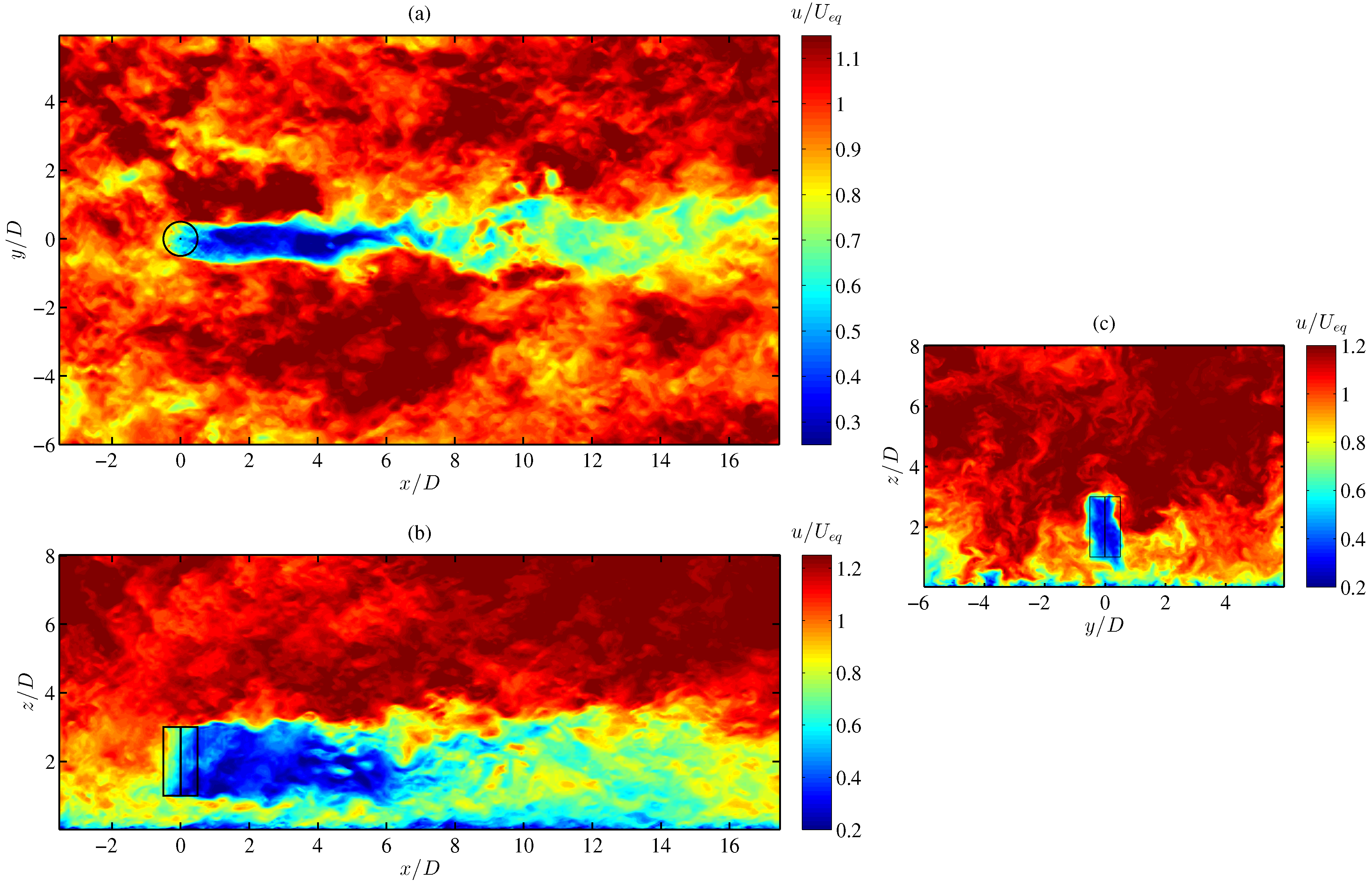
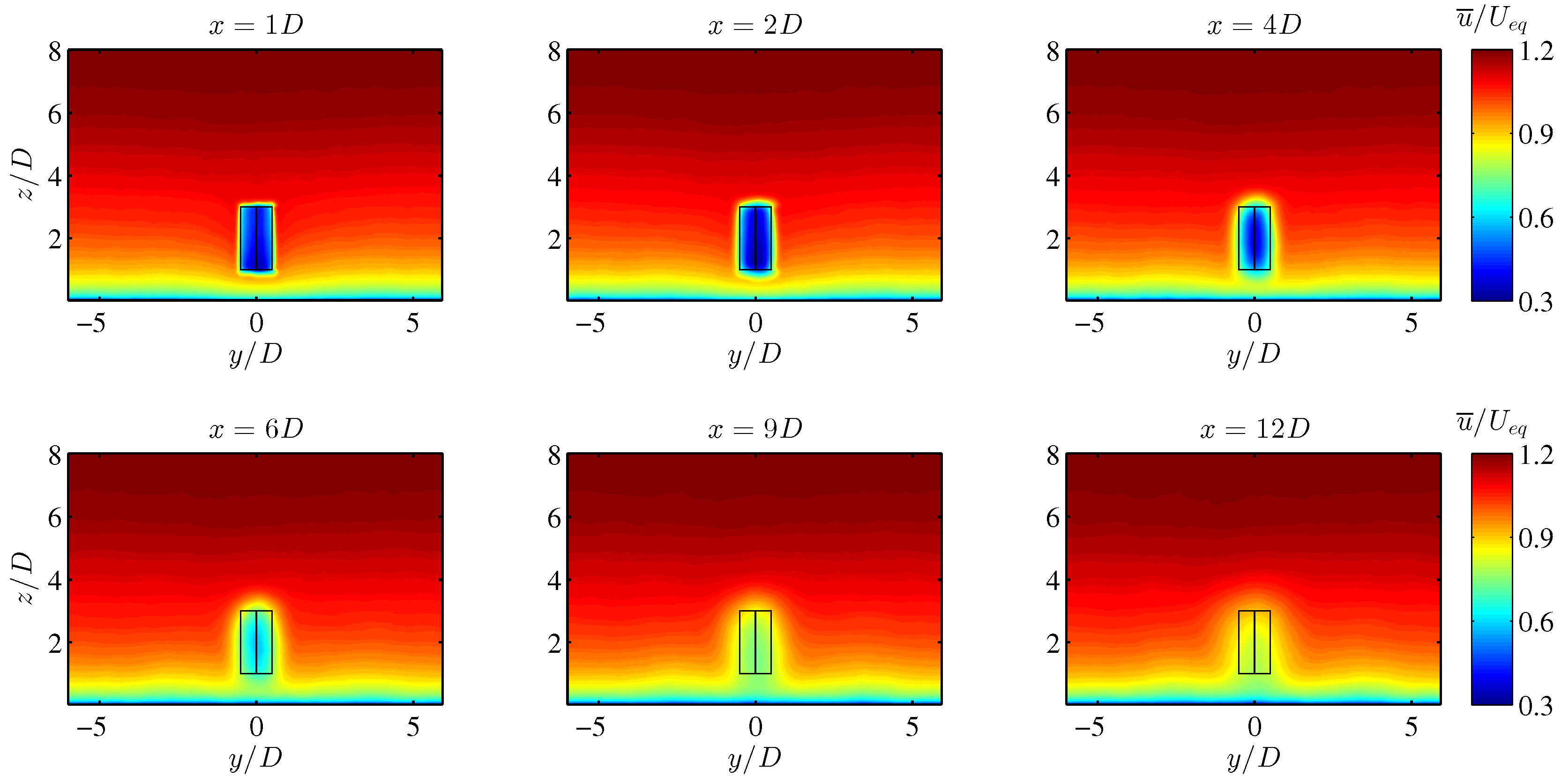
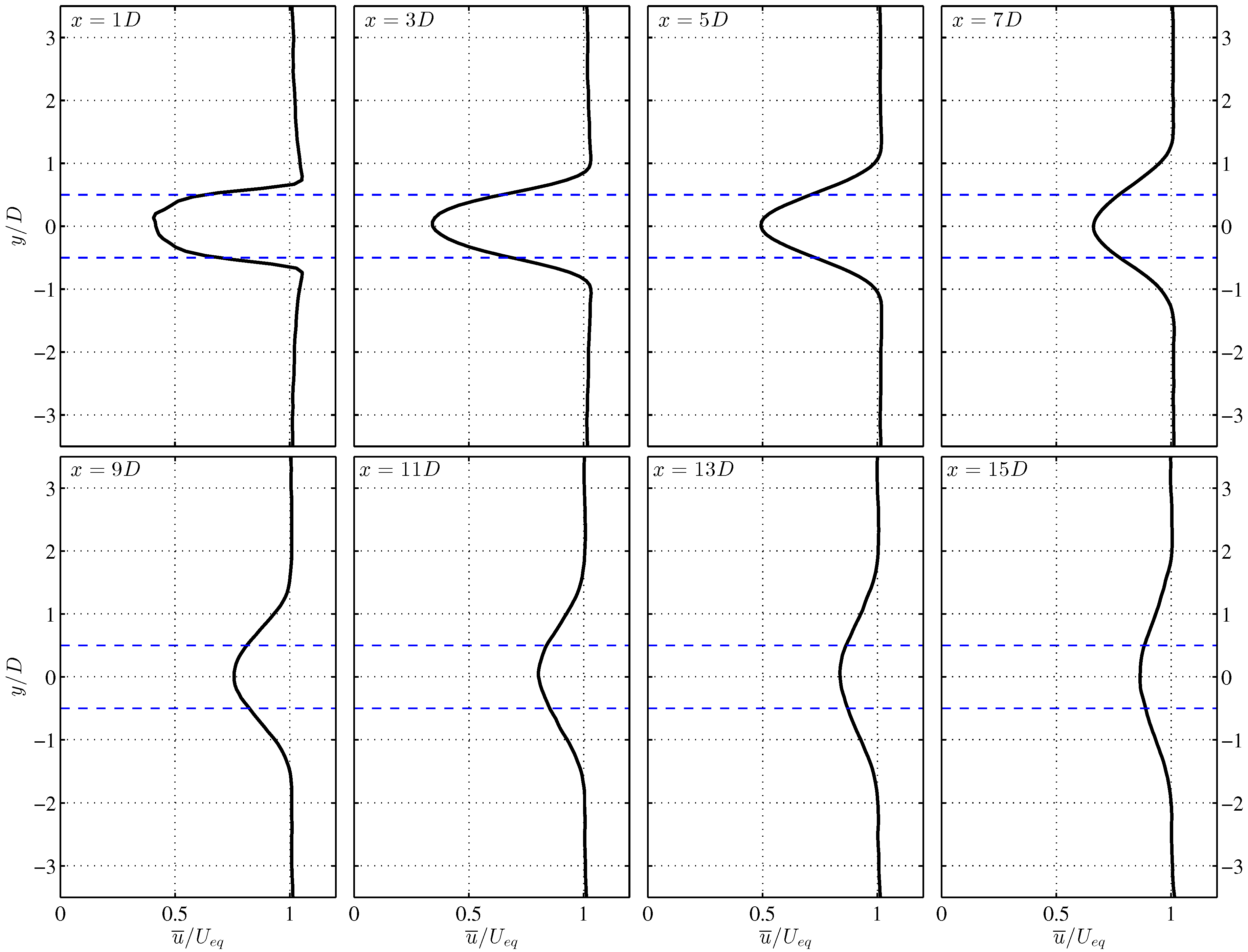
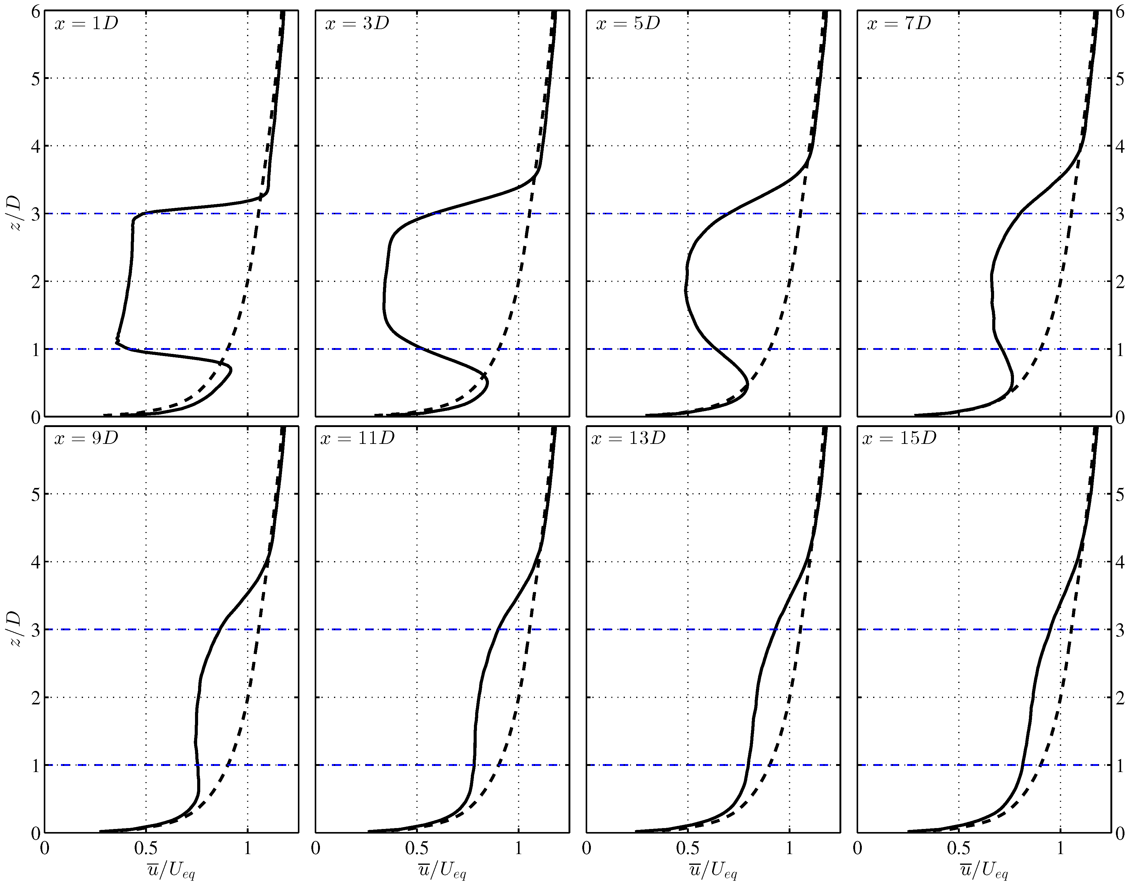
4.2. VAWT Wake
5. Summary
Supplementary Materials
Acknowledgments
Author Contributions
Conflicts of Interest
Appendix A

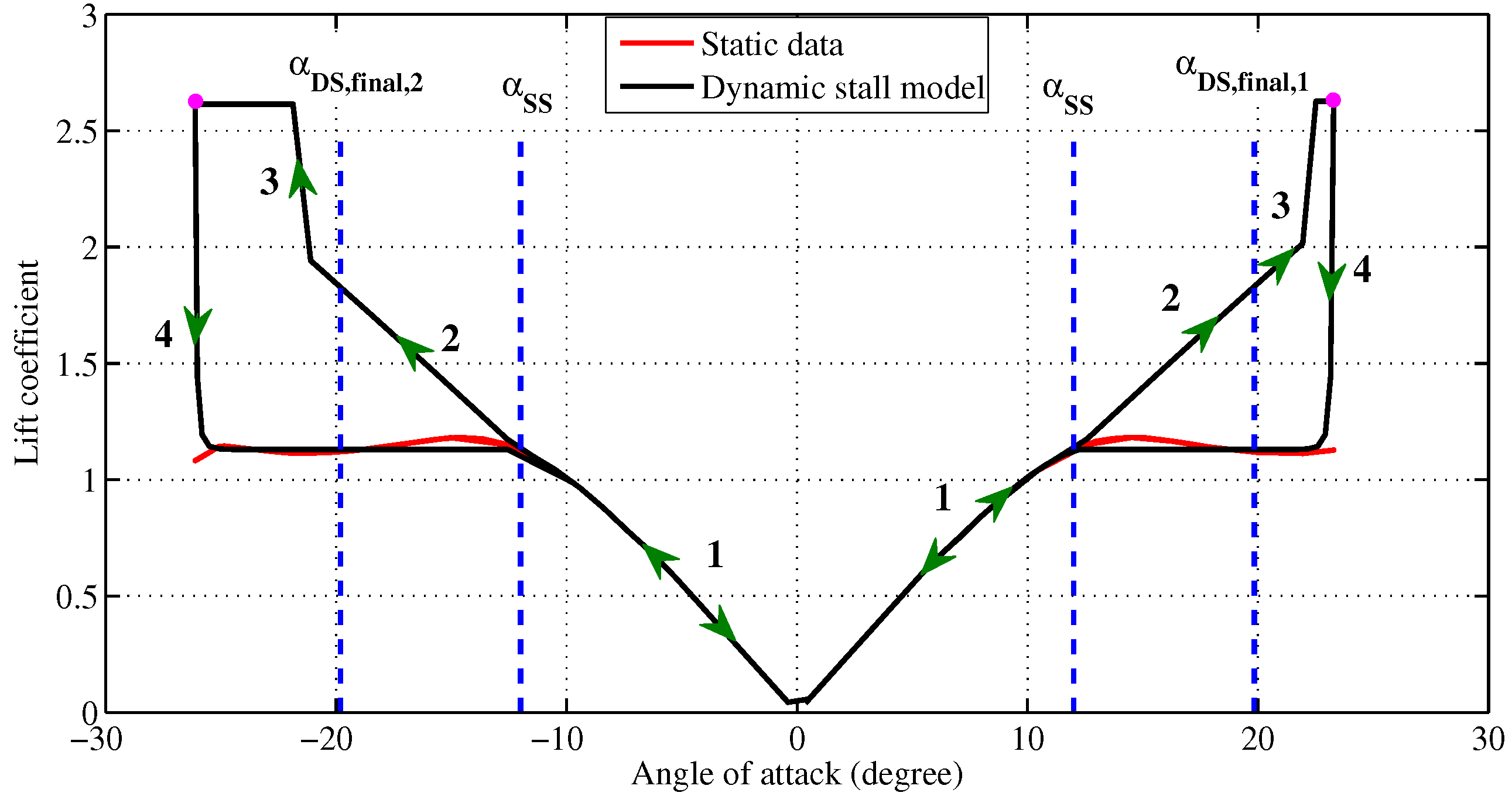
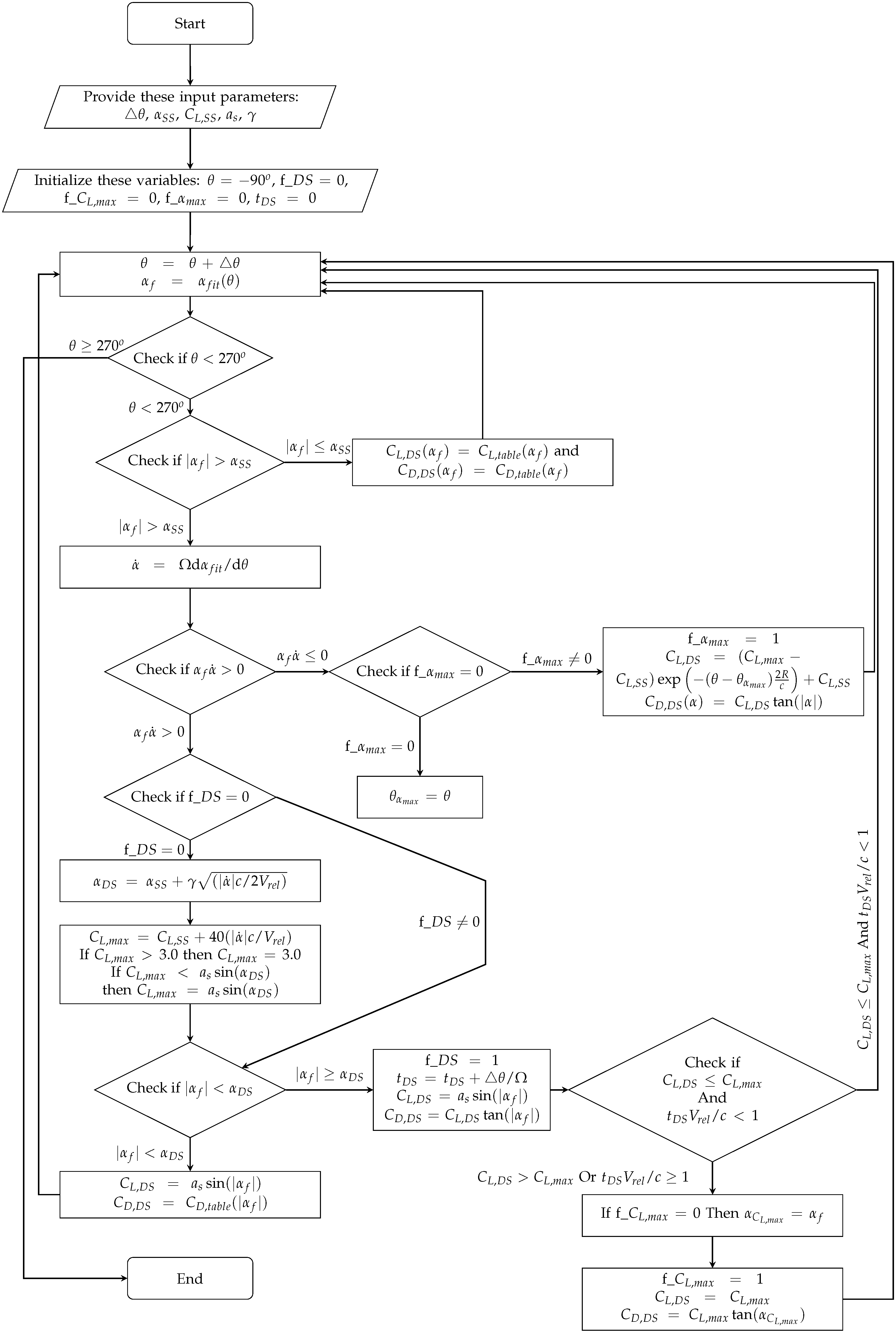
- State 1 occurs when . In this state, both lift and drag coefficients are extracted directly from the static tabulated airfoil data:
- State 2 occurs when and (i.e., is increasing in time). is calculated with the following formula:where c is the blade chord length, is the magnitude of the relative velocity (which is also a function of the azimuthal angle), , Ω is the angular velocity of the blade and γ is a constant that has a dimension of an angle and is weakly a function of the airfoil type and is determined experimentally [27]. If an experimental value for γ is not available, a value of one radian is recommended [31]. We keep calculating in this state, until the point at which is on the verge of becoming larger than (i.e., the point at which the model goes to State 3). We designate this last value of as , and with this value, we calculate the maximum value of (i.e., ):and we apply the following clipping conditions on :Throughout this state, the lift coefficient is extrapolated from static values, and the drag coefficient is still directly extracted from the static tabulated data:where (as in Noll and Ham [27]) a sine function is used for extrapolation (noting that in the range of angles of attack, on which we normally apply the model, is small, and we have ).
- State 3 occurs when and (i.e., is still increasing in time). As soon as the model enters State 3, we start to calculate the elapsed time from the moment in which State 3 is triggered; in other words, we start to calculate the time elapsed after the value has been reached; we call this time .In this state, the lift and drag coefficients are calculated as:However, in this state, we only keep using Equations (A8) and (A9) as long as these conditions are both satisfied: and ; otherwise, we set the lift coefficient to the value and calculate the drag coefficient accordingly (as shown below). We designate the value of of the moment in which either of the aforesaid conditions is on the verge of being violated as .
- State 4 occurs when and (i.e., when starts to decrease with time). We designate the azimuthal angle of the moment in which starts to decrease as . At this stage, is lowered exponentially (in time) from to .where R is the radius of the blade element about the axis of rotation (in the case of a VAWT, R is simply the radius of the VAWT rotor).
- (1) Tabulated airfoil data: and ; (2) ; (3) ; (4) ;
- (5) γ; (6) ; (7) ; (8) ; (9)


References
- Paraschivoiu, I. Wind Turbine Design—With Emphasis on Darrieus Concept; Polytechnic International Press: Montreal, QC, Canada, 2002. [Google Scholar]
- Tescione, G.; Ragni, D.; He, C.; Simao Ferreira, C.J.; van Bussel, G.J. Experimental and numerical aerodynamic analysis of vertical axis wind turbine wake. In Proceedings of the International Conference on Aerodynamics of Offshore Wind Energy Systems and Wakes, Lyngby, Denmark, 17–19 June 2013.
- Battisti, L.; Zanne, L.; Dell’Anna, S.; Dossena, V.; Persico, G.; Paradiso, B. Aerodynamic measurements on a vertical axis wind turbine in a large scale wind tunnel. J. Energy Resour. Technol. 2011, 133. [Google Scholar] [CrossRef]
- Bachant, P.; Wosnik, M. Characterising the near-wake of a cross-flow turbine. J. Turbul. 2015, 16, 392–410. [Google Scholar] [CrossRef]
- Araya, D.B.; Dabiri, J.O. A comparison of wake measurements in motor-driven and flow-driven turbine experiments. Exp. Fluids 2015, 56, 1–15. [Google Scholar] [CrossRef]
- Brochier, G.; Fraunie, P.; Beguier, C.; Paraschivoiu, I. Water channel experiments of dynamic stall on darrieus wind turbine blades. AIAA J. Propuls. Power 1986, 2, 445–449. [Google Scholar]
- Rolin, V.F.C.; Porté-Agel, F. Wind-tunnel study of the wake behind a vertical axis wind turbine in a boundary layer flow using stereoscopic particle image velocimetry. J. Phys. Conf. Ser. 2015, 625, 012012. [Google Scholar] [CrossRef]
- Ryan, K.J.; Coletti, F.; Elkins, C.J.; Dabiri, J.O.; Eaton, J.K. Three-dimensional flow field around and downstream of a subscale model rotating vertical axis wind turbine. Exp. Fluids 2016, 57, 1–15. [Google Scholar] [CrossRef]
- Castelli, M.R.; Englaro, A.; Benini, E. The darrieus wind turbine: Proposal for a new performance prediction model based on CFD. Energy 2011, 36, 4919–4934. [Google Scholar] [CrossRef]
- Pierce, B.; Moin, P.; Dabiri, J.O. Evaluation of Point-Forcing Models with Application to Vertical Axis Wind Turbine Farms; Annual Research Briefs; Center for Turbulence Research, Stanford University: Stanford, CA, USA, 2013. [Google Scholar]
- Shamsoddin, S.; Porté-Agel, F. Large eddy simulation of vertical axis wind turbine wakes. Energies 2014, 7, 890–912. [Google Scholar] [CrossRef]
- Rajagopalan, R.G.; Fanucci, J.B. Finite difference model for vertical-axis wind turbines. AIAA J. Propuls. Power 1985, 1, 432–436. [Google Scholar] [CrossRef]
- Rajagopalan, R.G.; Berg, D.E.; Klimas, P.C. Development of a three-dimensional model for the darrieus rotor and its wake. AIAA J. Propuls. Power 1995, 11, 185–195. [Google Scholar] [CrossRef]
- Shen, W.; Zhang, J.; Sørensen, J. The actuator surface model: A new navier-stokes based model for rotor computations. J. Sol. Energy Eng. 2009, 131. [Google Scholar] [CrossRef]
- Stoll, R.; Porté-Agel, F. Dynamic subgrid-scale models for momentum and scalar fluxes in large-eddy simulation of neutrally stratified atmospheric boundary layers over heterogeneous terrain. Water Resour. Res. 2006, 42. [Google Scholar] [CrossRef]
- Albertson, J.D.; Parlange, M.B. Surfaces length scales and shear stress: implications for land-atmosphere interactions over complex terrain. Water Resour. Res. 1999, 35, 2121–2132. [Google Scholar] [CrossRef]
- Porté-Agel, F.; Meneveau, C.; Parlange, M.B. A scale-dependent dynamic model for large-eddy simulation: Application to a neutral atmospheric boundary layer. J. Fluid Mech. 2000, 415, 261–284. [Google Scholar] [CrossRef]
- Porté-Agel, F.; Wu, Y.T.; Lu, H.; Conzemius, R.J. Large-eddy simulation of atmospheric boundary layer flow through wind turbines and wind farms. J. Wind Eng. Ind. Aerodyn. 2011, 99, 154–168. [Google Scholar] [CrossRef]
- Monin, A.; Obukhov, M. Basic laws of turbulent mixing in the ground layer of the atmosphere. Tr. Akad. Nauk SSSR Geophiz. Inst. 1954, 24, 163–187. [Google Scholar]
- Moeng, C. A large-eddy simulation model for the study of planetary boundary-layer turbulence. J. Atmos. Sci. 1984, 46, 2311–2330. [Google Scholar] [CrossRef]
- Stoll, R.; Porté-Agel, F. Effect of roughness on surface boundary conditions for large-eddy simulation. Bound. Layer Meteorol. 2006, 118, 169–187. [Google Scholar] [CrossRef]
- Tseng, Y.H.; Meneveau, C.; Parlange, M.B. Modeling flow around bluff bodies and predicting urban dispersion using large eddy simulation. Environ. Sci. Technol. 2006, 40, 2653–2662. [Google Scholar] [CrossRef] [PubMed]
- Wu, Y.T.; Porté-Agel, F. Large-eddy simulation of wind-turbine wakes: Evaluation of turbine parametrisations. Bound. Layer Meteorol. 2011, 138, 345–366. [Google Scholar] [CrossRef]
- Porté-Agel, F.; Wu, Y.T.; Chen, C.H. A numerical study of the effects of wind direction on turbine wakes and power losses in a large wind farm. Energies 2013, 6, 5297–5313. [Google Scholar] [CrossRef]
- Sheldahl, R.E.; Klimas, P.C. Aerodynamic Characteristics of Seven Airfoil Sections through 180 Degrees Angle of Attack for Use in Aerodynamic Analysis of Vertical Axis Wind Turbines; Technical Report SAND80-2114; Sandia National Laboratories: Albuquerque, NM, USA, 1981.
- Scheurich, F.; Brown, R. Effect of dynamic stall on the aerodynamics of vertical-axis wind turbines. AIAA J. 2011, 49, 2511–2521. [Google Scholar] [CrossRef]
- Noll, R.B.; Ham, N.D. Dynamic Stall of Small Wind Systems; Technical Report; Aerospace Systems Inc.: Burlington, MA, USA, 1983. [Google Scholar]
- Templin, R.J.; Rangi, R.S. Vertical-axis wind turbine development in Canada. IEE Proc. A Phys. Sci. Meas. Instrum. Manag. Educ. Rev. 1983, 130, 555–561. [Google Scholar] [CrossRef]
- Chen, T.; Liou, L. Blockage corrections in wind tunnel tests of small horizontal-axis wind turbines. Exp. Therm. Fluid Sci. 2011, 35, 565–569. [Google Scholar] [CrossRef]
- Ham, N.D. Aerodynamic loading on a two-dimensional airfoil during dynamic stall. AIAA J. 1968, 6, 1927–1934. [Google Scholar] [CrossRef]
- Hibbs, B.D. HAWTPerformance with Dynamic Stall; Technical Report SERI/STR 217-2732; AeroVironment, Inc.: Monrovia, CA, USA, 1986. [Google Scholar]


© 2016 by the authors; licensee MDPI, Basel, Switzerland. This article is an open access article distributed under the terms and conditions of the Creative Commons Attribution (CC-BY) license (http://creativecommons.org/licenses/by/4.0/).
Share and Cite
Shamsoddin, S.; Porté-Agel, F. A Large-Eddy Simulation Study of Vertical Axis Wind Turbine Wakes in the Atmospheric Boundary Layer. Energies 2016, 9, 366. https://doi.org/10.3390/en9050366
Shamsoddin S, Porté-Agel F. A Large-Eddy Simulation Study of Vertical Axis Wind Turbine Wakes in the Atmospheric Boundary Layer. Energies. 2016; 9(5):366. https://doi.org/10.3390/en9050366
Chicago/Turabian StyleShamsoddin, Sina, and Fernando Porté-Agel. 2016. "A Large-Eddy Simulation Study of Vertical Axis Wind Turbine Wakes in the Atmospheric Boundary Layer" Energies 9, no. 5: 366. https://doi.org/10.3390/en9050366