Short-Term Traffic State Prediction Based on Mobile Edge Computing in V2X Communication

Abstract

Real-time and reliable short-term traffic state prediction is one of the most critical technologies in intelligent transportation systems (ITS). However, the traffic state is generally perceived by single sensor in existing studies, which is difficult to satisfy the requirement of real-time prediction in complex traffic networks. In this paper, a short-term traffic prediction model based on complex neural network is proposed under the environment of vehicle-to-everything (V2X) communication systems. Firstly, a traffic perception system of multi-source sensors based on V2X communication is proposed and designed. A mobile edge computing (MEC)-assisted architecture is then introduced in a V2X network to facilitate perceptual and computational abilities of the system. Moreover, the graph convolutional network (GCN), the gated recurrent unit (GRU), and the soft-attention mechanism are combined to extract spatiotemporal features of traffic state and integrate them for future prediction. Finally, an intelligent roadside test platform is demonstrated for perception and computation of real-time traffic state. The comparison experiments show that the proposed method can significantly improve the prediction accuracy by comparing with the existing neural network models, which consider one of the spatiotemporal features. In particular, for comparison results of the traffic state prediction and the error value of root mean squared error (RMSE) is reduced by 39.53%, which is the greatest reduction in error occurrences by comparing with the GCN and GRU models in 5, 10, 15 and 30 min respectively.

1. Introduction

Due to considerable urbanization in recent years, the increasing number of vehicles in cities has led to various traffic problems such as traffic congestion, accidents and environmental degradation. According to the state-of-the-art, the main solutions to these problems lie in improving the traffic capacity of the road [1,2,3]. However, most studies concentrate on in-car advisory systems on lane, speed, and headway [4], strategies design on traffic networks [5], and different model managements [6]. Traditional single-component sensors are difficult to meet the predicted requirements of complex traffic networks. Therefore, more efficient and effective approaches still need to be explored to improve the traffic capacity. Along with the development of communication technologies, the mobile communication networks are expected to be established in people, vehicles, and roads for transforming and transferring real-time information accurately. Vehicle-to-everything (V2X), fusing on various vehicles and roads information, has been treated as the core technology for the next generation of intelligent transportation system (ITS) to perceive real-time traffic state on the roads [7], which faces huge real-time data processing problems in transmission quality. In order to solve the problems, in this paper, an ITS is proposed by integrating vehicles and roads with wireless communication technologies for flexible information sharing and accurate traffic state prediction. The delay of data transmission can be greatly reduced and the efficiency of data processing can then be effectively improved with the constructed mobile edge computing (MEC) platform in V2X network [8]. The development of these technologies plays a key role in the short-term traffic state prediction, which involves the information of vehicle driving state, road environment, and other traffic state messages. Through the support of these technologies, the efficient traffic state management can be guaranteed.

The short-term traffic state prediction has been conducted in many studies, which refers to the next stage of traffic state prediction with no more than 30 min [9]. The employed approaches can be divided into two types: model-driven oriented and data-driven oriented. The model-driven methods describe the traffic state by building a macroscopic model, which mainly includes various Kalman filtering algorithms [10], and the data-driven method extracts spatiotemporal features from historical traffic data and applies deep learning to predict the traffic state [11]. Based on our intensive investigations, the data-driven method, as the main means for traffic state prediction, is utilized in most of the research. Lv et al. [12] proposed a traffic flow prediction method based on deep learning by considering the spatiotemporal correlation of traffic flow, where an automatic encoder model was used to learn general traffic flow characteristics and train them in a hierarchical manner. This work was the first opportunity to use an automatic encoder as a building block to represent a deep architectural model for predicting traffic flow characteristics. Li et al. [13] established a depth neural network based on long short-term memory (LSTM) to predict traffic flow during peak hours. This method identified the unique characteristics of traffic data, and further improved the prediction model of mixed depth LSTM model. However, these models rarely take the spatial feature of the traffic network into account. Moreover, convolution neural network (CNN) and recurrent neural network (RNN) are widely applied to a variety of machine learning tasks because of their strong hierarchical feature learning ability [14]. They are widely used in the fields of computer vision [15], natural language processing [16], and time series data prediction [17]. RNN and its variant model, such as the gated recurrent unit (GRU), can effectively extract temporal dependencies [18]. However, CNN model, regarding spatial relations as simple Euclidean structures, is not suitable for dealing with traffic networks with spatiotemporal characteristics. To solve the above shortcomings, the graph convolution neural network (GCN) displayed in CNN is extended in [19]. Cui et al. [20] realized GCN through an adjacency matrix based on the traffic network topology and identified the most influential road sections in the traffic network. However, the adjacency matrix was heuristic, which reflected that the spatial relationship between the vertexes of the road network is not accurate. In order to make up for the shortcomings of the graph convolution model based on heuristic adjacency matrix, Ye et al. [21] proposed a self-learning adjacency matrix and designed different adjacency matrices on different convolution layers. However, the use of multiple convolution layers in the traffic network will lead to the lack of explanation of the spatial relationships. Ma et al. [22] proposed a traffic learning model based on GCN. In this model, the traffic flow was learned as an image, and the spatiotemporal traffic dynamics were transformed into a two-dimensional spatiotemporal matrix, which can describe the spatiotemporal correlations of traffic flow. Li et al. [23] proposed three-channel networks, including GCN, GRU, and fully connected neural network (FCNN) to extract spatial, temporal, and other features, respectively.

Based on the above investigations, the challenges of traffic state prediction can be summarized as follows:

• How to perceive and predict traffic state in real time. The traditional traffic sensors are difficult to meet the predicted requirements of short-term traffic state prediction, especially for the accuracy requests of intelligent connected vehicles (ICVs).
• How to perceive and analyze the dynamic data of vehicles. The vehicles running on the road may face all kinds of sudden traffic incidents. However, traditional vehicular dynamic data strategies (such as floating vehicle) are difficult to meet the requests of accurate prediction in real time.
• How to effectively analyze and filter spatiotemporal features of traffic state. The spatiotemporal features of the traffic state are high nonlinear correlations, which are still the focus problems of urban traffic research. For example, the variation of traffic flow at one intersection will affect the traffic state at the adjacent intersection, meanwhile, affect the future traffic state over time.

To solve the above problems, this paper proposes a traffic perceptual and computational system, which incorporates the roadside intelligent sensors, ICVs, and traffic signal controller at the intersection. It can accurately perceive not only each single vehicular state, but also the whole intersection traffic state. The main contributions of the paper can be summarized as follows:

• Firstly, this paper proposes a traffic perceptual and computational system based on the MEC architecture, in which each edge server is responsible for managing the data upload of vehicles within its service scope. Moreover, the MEC server will predict traffic state based on the perceptual information.
• Secondly, this paper applies on board unit (OBU) data of ICVs to predict traffic state by tracking vehicular driving state in real time, which can effectively improve the accuracy of prediction.
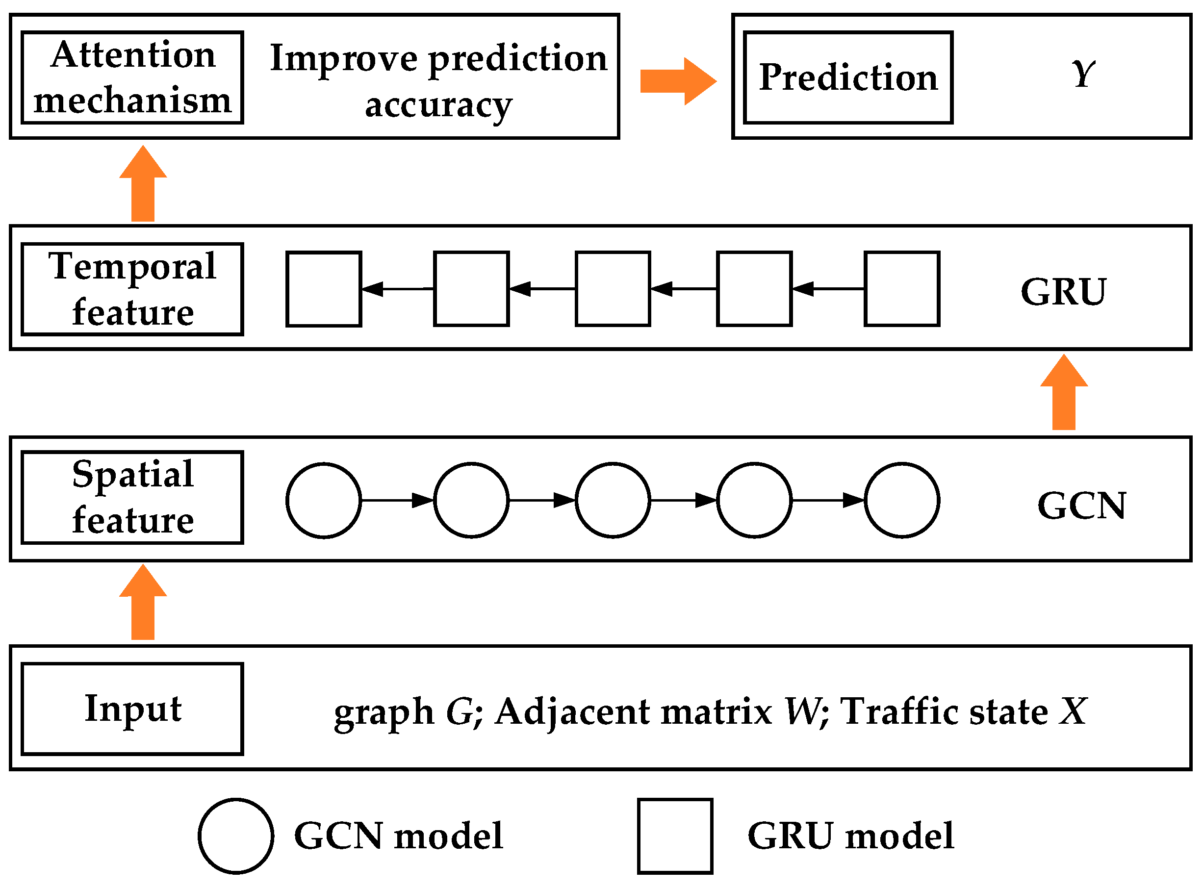
• Thirdly, with the characteristics of the MEC, this paper designs a traffic prediction model to analyze and evaluate the traffic state at the intersection in V2X environment. GCN and GRU models are combined to analyze spatiotemporal features of traffic data in the model. Then, the soft-attention mechanism is utilized to integrate the various extracted features.

The reminder of this paper is organized as follows. The traffic state perception system of an intersection scenario, which is based on MEC architecture in V2X communication, is described in Section 2, where a predicted model of short-term traffic state is then constructed and clarified. Section 3 presents experimental results and demonstrates the effectiveness of the proposed method. Finally, the conclusion is provided in Section 4.

2. Materials and Methods

The framework of the proposed method is described in Figure 1, which consists of a traffic perception system based on V2X, an edge computing module, and a traffic state prediction output module. Traffic states from various perception sources, such as roadside sensors, OBU, and traffic signal controller, can be collected by traffic perception system based on V2X. These states will then be delivered to a MEC server for further processing. Through graph constriction of intersection network, spatiotemporal feature analysis and soft-attention mechanism, the short-term traffic state at the intersection based on fusion results of V2X multi-source sensors can be accurately depicted and predicted. The involved modules are described in Section 2.1, Section 2.2 and Section 2.3.

2.1. Traffic State Perception

Traffic state is an unevenly distributed and complex random variable related to time variation. At the micro-level, the traffic state perception can be regarded as perceiving the behavior state of each vehicle, and at the macro-level, as the flow, speed, density, etc. in traffic scenarios. In this section, a traffic state perception system based on V2X communication will be introduced, and the perceptual information of traffic state will be analyzed.

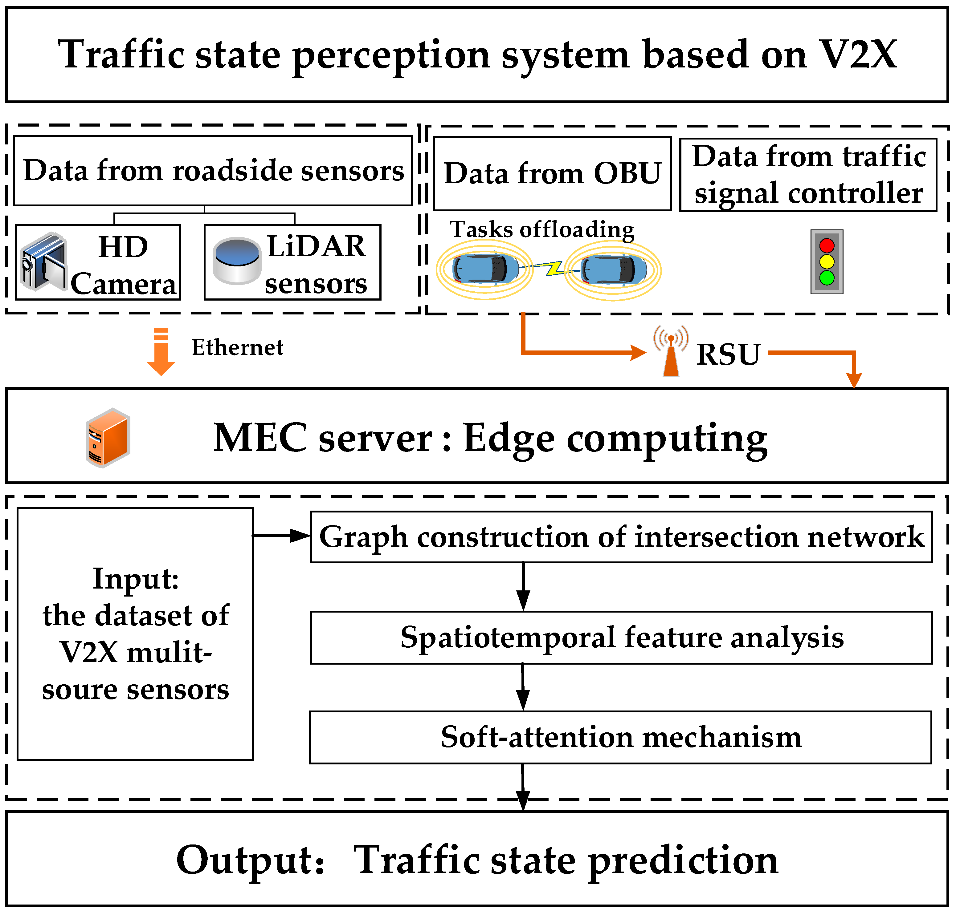
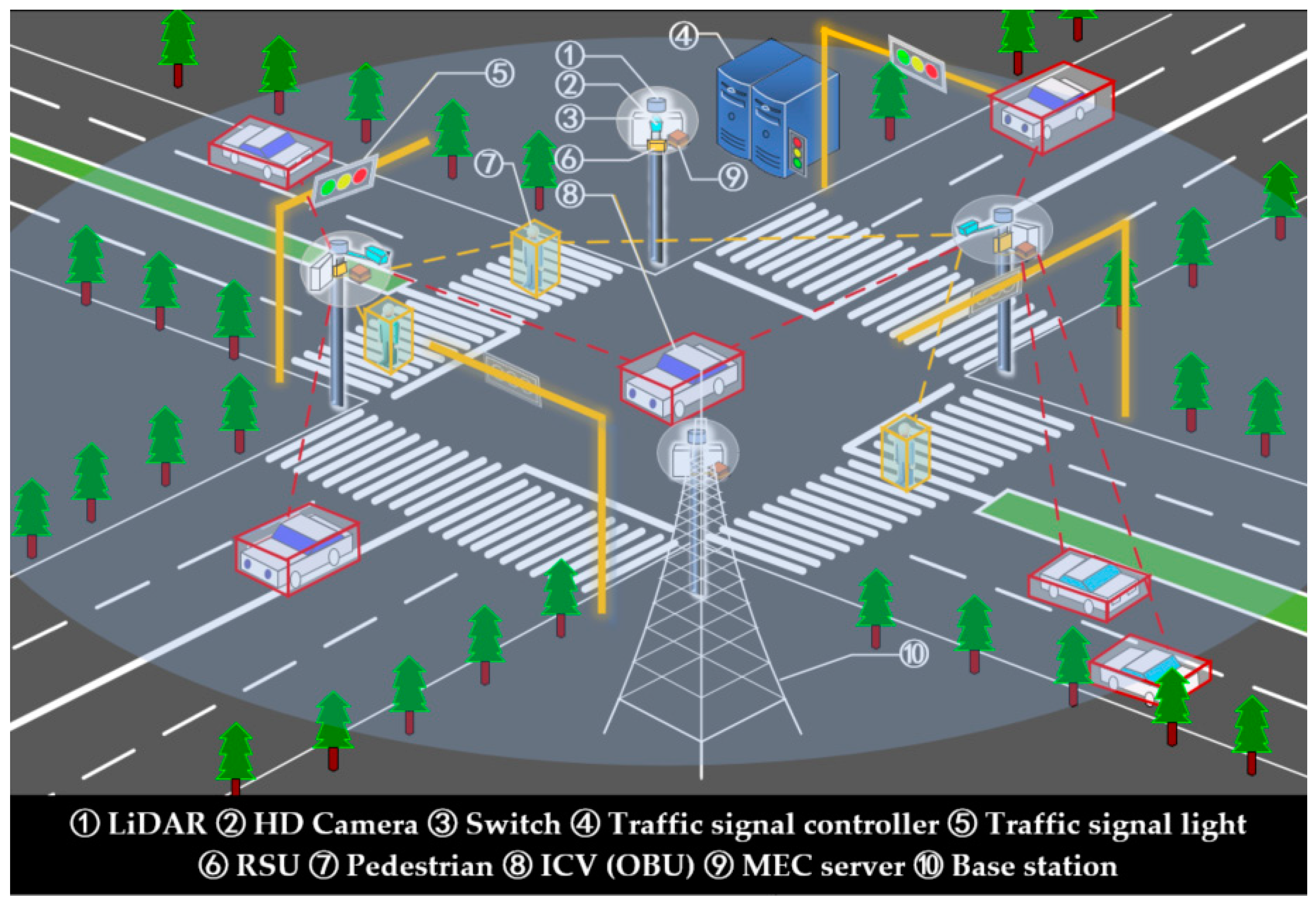
2.1.1. Traffic Perception System Based on V2X Communication

At an urban intersection, the traffic state usually refers to the driving state of all vehicles, which has the characteristics of dynamic, periodicity, randomness, etc. With the development of V2X communication technologies, the traffic state is generally perceived by the fusion of multi-source traffic sensors, then the information can be fed back to the users of other subsystems such as traffic management system (TMS) [24]. Finally, the perceived traffic information can be used to solve traffic and ICVs problems for ITS.

To improve the traffic efficiency, a traffic perception system based on the V2X communication technology is designed by taking advantages of low delay, high reliability, and high security of the V2X in this paper. As shown in Figure 2, intelligent roadside infrastructures mainly include LiDAR sensors, high definition (HD) cameras, intelligent roadside units (RSUs), switches, traffic signal light controllers, intelligent OBUs with V2X communication functions, a shared base station, and a series of MEC servers. In the perception database at the intersection of this system, the perception data are distributed, dynamic, heterogeneous, and spatiotemporal. Average traffic flow and mean speed capacity are chosen to be predicted and evaluative indicators of traffic state, then the comprehensive analyses are shown in the following parts.

2.1.2. Traffic Perception Data

The purpose of our system is to construct a stereoscopic and accurate perception database of the intersection. By comparing our system with the traditional traffic perception methods, the performance of the constructed system will be observed that whether it can realize more complex information interaction between vehicles and roads, and perceive the driving status of a single vehicle and roadside traffic environment information.

In ITS and cooperative vehicle infrastructure systems (CVIS), the traffic management department monitor the real-time traffic state by a variety of advanced sensors. Therefore, fusing more than two traffic sensors of data can provide more efficient, reliable, and accurate results. The fusion information of the system is reflected in feature-level data fusion, which is from roadside sensors, intelligent OBUs, and traffic signal controllers. The types and sources of the traffic perception data in this system are shown in

Table 1. Types and sources of traffic perception data.

Data Sources	Data Types
Roadside sensors	Vehicle information: license plate number, latitude, longitude, speed, horizontal distance, heading angle, etc.
	Traffic state information: average vehicular speed, average traffic flow, average queue length, parking line location, etc.
OBU	Timstamp, latitude, longitude, speed, acceleration, license plate number, wheel speed, steering angle, braking status, etc.
Traffic signal controller	Signal cycle, signal phase, traffic light color, remaining time of green, etc.

.

1.

Data from Roadside Sensors

In the system, roadside sensors include LiDAR sensors and cameras, by which real-time states of each target within the range of the sensors at the intersection can be easily obtained. To prevent the impact of pedestrians and other traffic participants, vehicles at the intersection are selected as targets to predict the traffic state in this system.

Based on the data fusion of the point cloud and the image, the accurate information of each vehicle, including the license plate number, the latitude, the longitude, the speed, the horizontal distance, the heading angle, and so on, can be perceived. Moreover, LiDAR sensors and cameras can also perceive the traffic state of the intersection, including the average vehicle speed, the average traffic flow, the average queue length and the parking line location.

2.

Data from OBU

OBU data consist of the real-time information of ICVs while driving at the intersection. Therefore, millions of observations and terabytes of data are generated every day [25]. In this system, the recorded information from OBU contains an anonymous identifier (ID), the timestamp, the GPS position (latitude, longitude), the speed, the acceleration, the license plate number, the wheel speed, the steering angle, and so on. Additionally, OBU data includes vehicular braking states.

3.

Data from Traffic Signal Controller

Traffic signal control is a fundamental element in traffic guidance at urban signalized intersections [26,27]. The core of the integration between traffic signal control and traffic guidance is in temporal and spatial synchronization [28]. At the macro level, traffic signal control can actively guide the drivers to choose the path by combining the traffic guidance information to balance the traffic pressure. At the middle and micro level, the spatial variables, such as the number of lanes, lane functions, and traffic flow directions, are combined with the temporal variables to achieve more efficient traffic optimization, including green signal ratio, phase sequence and phase difference of signal light. In our system, the signal cycle, the signal phase, the traffic light color, the remaining time of green, etc., are involved in the traffic signal controller.

2.2. MEC Architecture

MEC architecture can extend the cloud computing services to the edge of networks according to the white paper proposed by European Telecommunications Standards Institute (ETSI). In our system, edge computing provides a service environment with high bandwidth and low latency in tasks offloading from mobile vehicles to MEC servers. The MEC architecture of this system includes three modules, which are cloud module, roadside module, and on-board module, as described in Figure 3. In this paper, roadside computing resources provided by the MEC architecture can meet the computing demands.

As shown in Figure 3, the roadside module is the perceptual part of the system, where LiDAR sensors and HD cameras are wired to the MEC server through the switch, and the ICVs are connected with traffic signal controllers based on V2X communications provided by RSU. The cloud module can store the historical traffic data from roadside sensors and provide cloud computing services. The on-board module refers to ICVs with OBUs, which can upload their own messages to the MEC server by task offloading strategy. Specifically, in the MEC architecture, ICVs can receive application-oriented information and upload messages to MEC server via PC5 interface. The service schedule is described in Figure 4.

In Figure 4, the MEC server is responsible for dealing with the uploaded data of vehicles in the local server, which includes data acquisition and traffic state prediction. The MEC server can be integrated into the strategy development of vehicular data acquisition. The process of data acquisition can be described as:

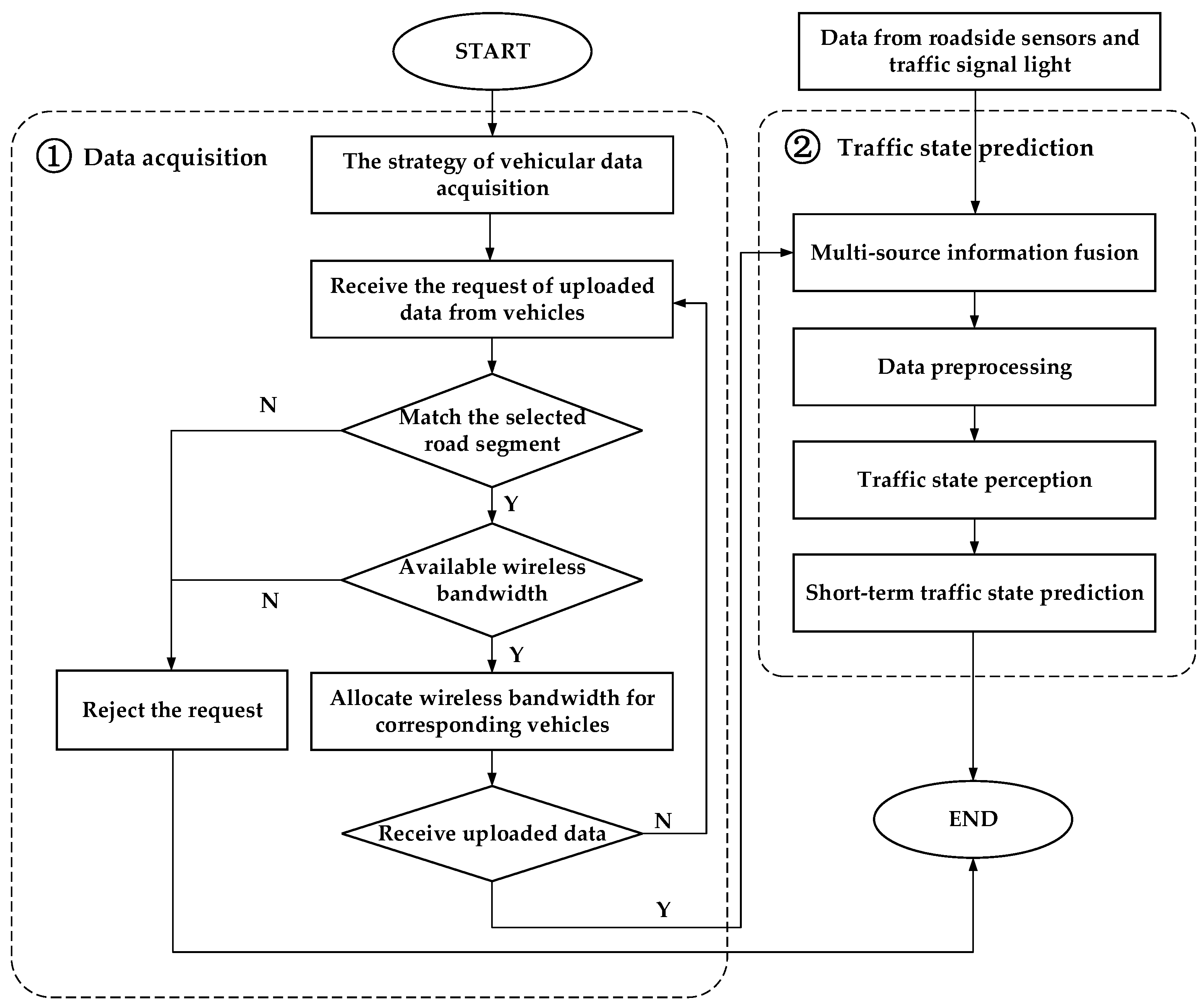
• Firstly, the MEC server can decide whether the requests of data uploading can be received by listening to messages broadcast from vehicles. These messages include the required bandwidth of the vehicle and the section ID associated with the vehicle.
• The MEC server will check if the ID of the corresponding section is selected. If the ID does not match, the MEC server rejects the request; otherwise, if the ID matches, the actions proceed to the next step.
• The MEC server then checks whether the required bandwidth can be met. If not, the MEC server rejects the request; if yes, the MEC server allocates bandwidth to the vehicle.
• Finally, the MEC server is ready to receive the uploaded vehicle data. If the data is uploaded successfully, the MEC server updates the allocated bandwidth of the corresponding road section. Otherwise, the allocated bandwidth will not be updated.

As for the traffic state prediction, the MEC server can fuse the actual traffic state based on the uploaded messages of vehicles and multi-source information of roadside sensors. The process can be depicted as:

• Firstly, multi-source information can be fused by the MEC server.
• Then, the MEC server processes the original vehicular data, including eliminating invalid data and sensing the traffic state information based on vehicular data.
• Finally, by designing a model of short-term traffic state prediction, the MEC server can predict the traffic state of the intersection of the system.

2.3. The Model of Short-Term Traffic State Prediction

Considering the temporal and spatial features of traffic states, a short-term traffic state prediction model is designed. As shown in Figure 5, the framework is divided into five modules: input module, temporal feature module, spatial feature module, attention mechanism module, and prediction module.

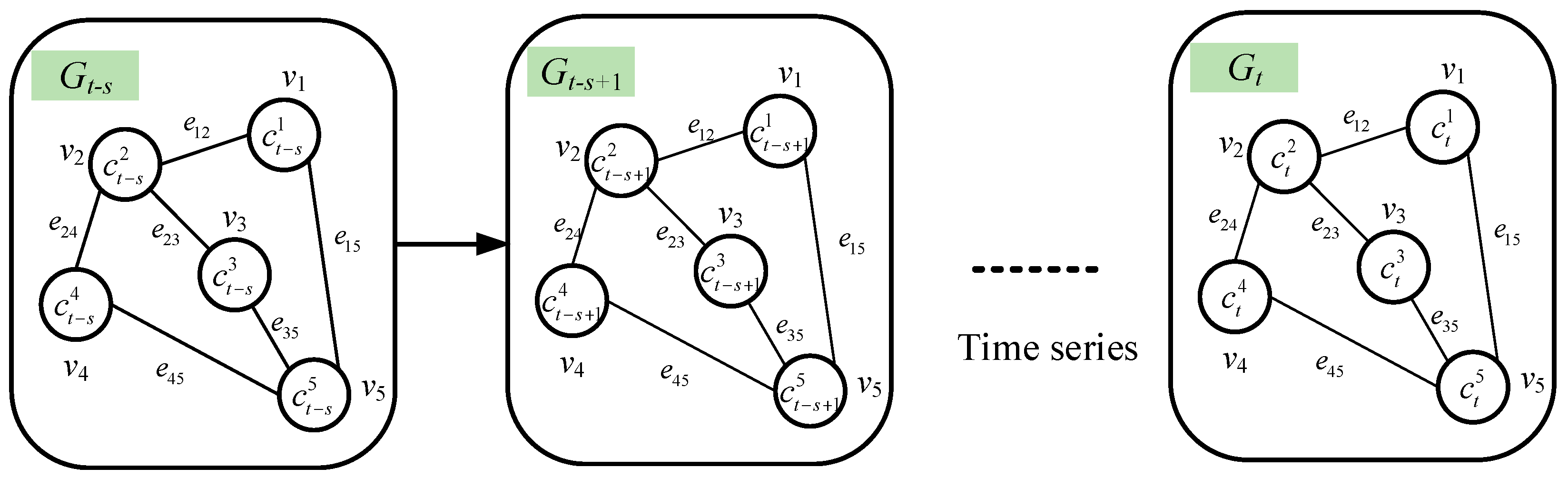
2.3.1. Graph Construction of Intersection Network

In the network of urban intersection, vertexes can represent a series of traffic features, which usually include vehicular speed, acceleration, position, and other vehicular state information.

As shown in Figure 6, the network of intersection at different times can be described as $G=\{V,E,W\}$. In the graph G, each vertex is treated as a vehicle, and V is a set of vehicle vertexes, $V=\{v_1,v_2,\dots ,v_N\}$, where N represents number of vertexes; E is a set of edges, where $e_{ij}\in E$. $\mathit{W}$ is the adjacent matrix, which represents the connection between vehicles, $\mathit{W}\in R^{N\times N}$. Adjacent matrix is the basis for exploratory analysis of the spatiotemporal correlation of traffic flow at the intersection network. The adjacency matrix is described by a binary matrix [0, 1], where 0 stands for there being no link between two edges, and 1 denotes that there is a link.

In Figure 6, each vertex in networks has actual attributes including speed, acceleration and other vehicular information, and can be expressed as $C_t=\{c_t^1,c_t^2,\dots ,c_t^N\}$, $C\in R^{N\times P}$, where $c_t^i$ represents the attribute of the vertex v_i at time t and P represents the number of vertex attributes. The attributes of the vehicle vertex in the network can be obtained from V2X environment. Therefore, $x_t\in R^{N\times K}$ is used to represent the traffic state at the time t at the intersection, where K is the number of traffic state attributes, including traffic flow, traffic speed, traffic density and queuing length.

According to the characteristics of urban intersections, the mean speed capacity $M_v$ and the average traffic flow $Q_t$ are selected to be indexes to describe traffic sates at the intersection. The mean speed capacity is defined as shown in Equations (1) and (2).

$$\overline{V}=\frac{{\displaystyle {\sum }_{t=1}^k{\overline{v}}_t}}{k}$$

(1)

$$M_v=\frac{\overline{V}}{v_{\max }}$$

(2)

where $\overline{V}$ is the mean speed of all vehicles at the intersection in time k, and $v_{\max }$ is the limitation maximum speed in time k. $M_v$, as the mean speed capacity, is positively correlated with the performance of traffic state; thus, it is also used to evaluate the traffic state at an intersection. The threshold of $M_v$ is set to 0.6 for a standard traffic sate in [29].

Therefore, the problem of short-term traffic state prediction can be described as: in the given s historical time steps, the vehicular observation value of N vertexes in graph G is $\{C_{t-s},C_{t-s+1},\dots ,C_t\}$, and the traffic state is $X_t^s=\{x_{t-s},x_{t-s+1},\dots ,x_t\}$. Then at the next time step T, the predicted value set of all vertexes in graph G is $Y_t^T=\{x_{t+1},x_{t+2},\dots ,x_{t+T}\}$, as shown in Equation (3). The f function is mapped to learn the spatiotemporal features of the traffic state.

$$Y_t^T=f(G;X_t^s)$$

(3)

where s is the length of historical time series, T is the length of time series that need to be predicted.

2.3.2. Spatial Feature Extraction

An intersection is defined as the structure of the road network graph, and the GCN model is more sensitive to traffic spatial features. The GCN model can deduce its own vertex information by using the information of the surrounding vertexes and its own original information. Therefore, in the graph of intersection, both vertex information and structure of graph should be integrated for consideration. The GCN model can learn not only the characteristics of vertexes automatically, but also the correlation information between any of two vertexes.

The convolutional neural (CN) model is an operation which convolves on the graph by the Fourier transform. The advantage of the GCN model is to extract spatial features by the neighborhood information of vertexes. According to the corresponding changes of graph convolution in [30], the most important graph convolution can be obtained, as shown in Equation (4):

$$g\ast h=U({\mathit{u}}^{T}g·{\mathit{u}}^{T}h)$$

(4)

where g is convolution kernel function, $h$ is graph signal on each vertex, and $h=\left[h\left(1\right), h\left(2\right),\dots ,h\left(n\right)\right]$. u is not only the basis of Fourier transform, but also the eigenvector of Laplace matrix. In particular, the more complicated the traffic situation becomes, the higher the computational complexity when the Laplace matrix is decomposed.

According to [31], the function f can be used Chebyshev polynomials for k-order approximation. The recursive function of Chebyshev polynomial is expressed as

$$\begin{array}{c}{T}_k(x)=2x{T}_{k-1}(x)-T_{k-2}(x)\\ T_0=1\\ T_1(x)=x\end{array}$$

(5)

where k is the order of Chebyshev expansion.

On the spectral graph, the approximate solution is carried out by Chebyshev polynomials, and the effect is equivalent to calculate the characteristic of each vertex by extracting the information of the 0~(k − 1)-th order neighbors of each vertex in the graph. Therefore, the output of the (l + 1)-th layer $H^{l+1}$ in GCN can be written as

$${\mathit{H}}^{l+1}=\sigma ({\tilde{\mathit{D}}}^{\raisebox{1ex}{$1$}\!\left/ \!\raisebox{-1ex}{$2$}\right.}\tilde{\mathit{W}}{\tilde{\mathit{D}}}^{\raisebox{1ex}{$1$}\!\left/ \!\raisebox{-1ex}{$2$}\right.}{\mathit{H}}^{(l)}{\theta }^{(l)})$$

(6)

where $\tilde{\mathit{W}}=\mathit{W}+{\mathit{I}}_N$ is the matrix with added self-connections, ${\mathit{I}}_N$ is the identity matrix, $\tilde{\mathit{D}}={\displaystyle {\sum }_j{\tilde{\mathit{W}}}_{ij}}$ represents the degree matrix, ${\mathit{H}}^{(l)}$ is the output of the layer, ${\theta }^{(l)}$ is the parameter of the layer, and $\sigma (·)$ represents the sigmoid function for a nonlinear model.

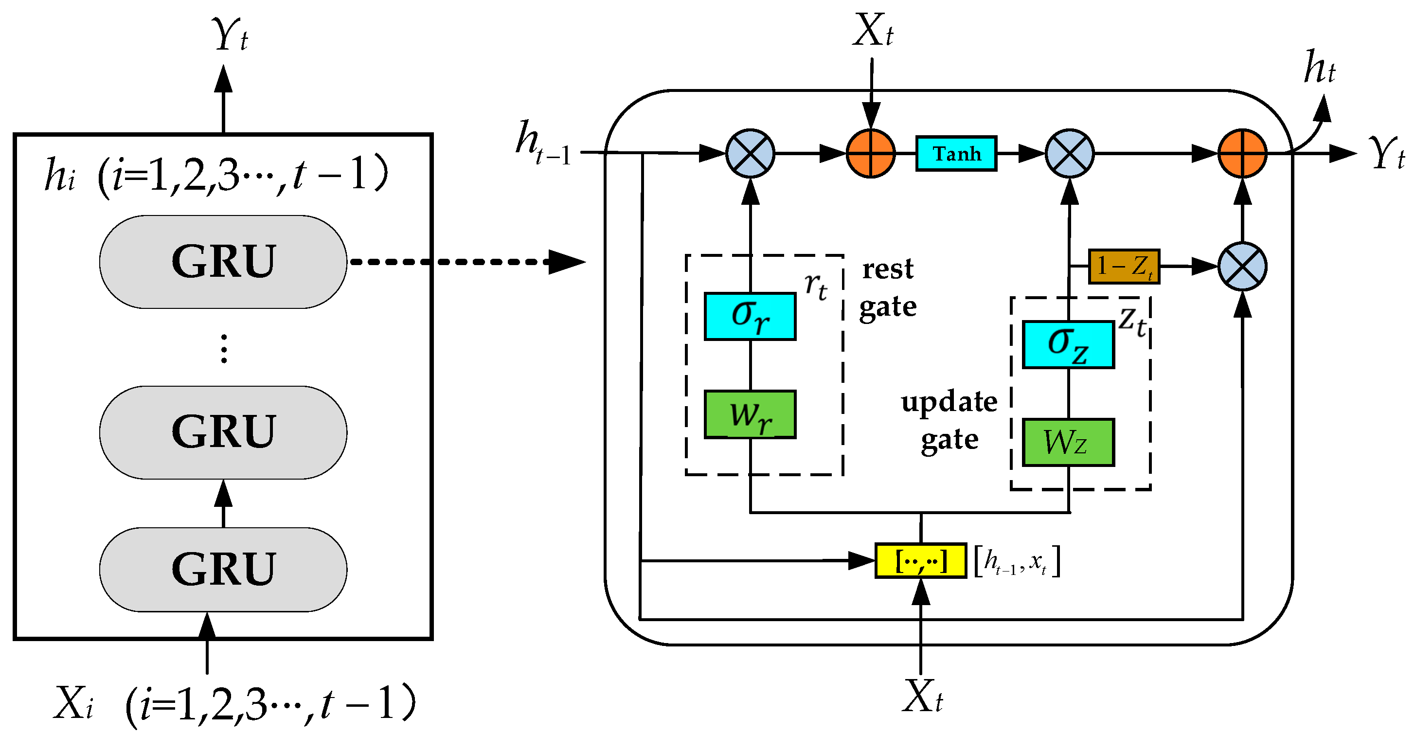
2.3.3. Temporal Feature Extraction

The variation in traffic over time is usually nonlinear and unstable. LSTM model, as the most extensive network, is used to deal with time series-related problems. The GRU is proposed based on LSTM. Compared with LSTM, the GRU model has a simpler structure, smaller parameter values and faster training speeds. The GRU model can effectively deal with short-term information with gated mechanism for different task processes.

As shown in Figure 7, the structure of GRU contains an update gate z_t, a rest gate r_t, and a memory unit h_t. The reset gate is used to control the degree of ignoring the status information of the previous moment. The update gate is used to control the state information of the previous moment, so that the useful information can be brought into the current state.

The states of update gate, rest gate, and memory unit are defined as follows:

$$z_t=\sigma ({\mathit{W}}_z·\left[h_{t-1},x_t\right])$$

(7)

$$r_t=\sigma ({\mathit{W}}_r·\left[h_{t-1},x_t\right])$$

(8)

$${\tilde{h}}_t=\tanh ({\mathit{W}}_h·\left[r_t\otimes h_{t-1},x_t\right])$$

(9)

$$h_t=(1-z_t)\otimes h_{t-1}+z_t\otimes {\tilde{h}}_t$$

(10)

where $x=\{x_1,x_2,\dots ,x_t\}$ is the output of the GCN model, which has extracted spatial features of the traffic data. ${\mathit{W}}_z$, ${\mathit{W}}_r$ and ${\mathit{W}}_h$ represent the weight matrixes of z_t, r_t and h_t respectively. $\sigma (·)$ and $\tanh (·)$ are the two activation functions, which can be defined as

$$\sigma =\frac{1}{1+e^{-x}}$$

(11)

$$\tanh =\frac{e^x-e^{-x}}{e^x+e^{-x}}$$

(12)

In summary, the GCN model is used to extract the topological structure of intersection for obtaining spatial features. The GRU model is used to extract the dynamic variation of traffic state in the network for obtaining temporal features.

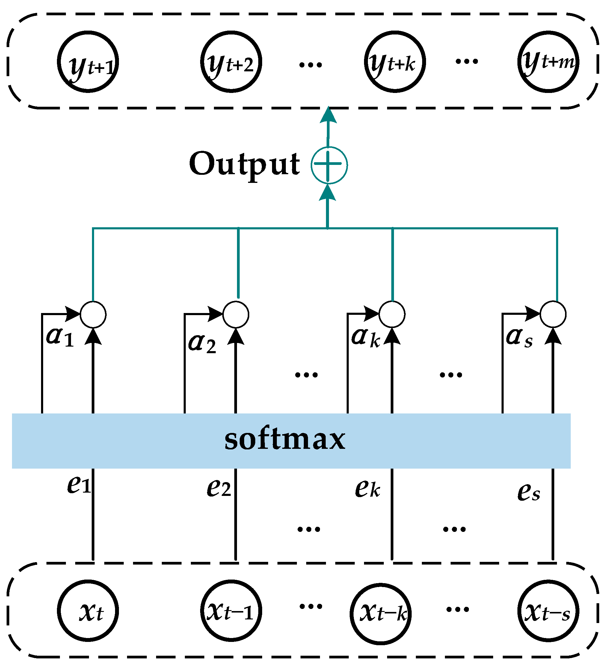
2.3.4. Attention Mechanism Module

To make use of the spatiotemporal characteristics of the historic traffic state at urban intersection, the short-term prediction of traffic state is carried out through the redistribution of weight by attention mechanism. First, the attention coefficient of each time series needs to be calculated for the predicted target. Then these coefficients are used to evaluate the prediction results. Finally, when predicting the traffic state, the state values of vertexes with stronger correlation are calculated by the soft-attention mechanism.

The structure of the attention mechanism is shown in Figure 8, where the output of the last layer of GRU model is the input of the soft-attention mechanism. For different time series, the weight of each time series feature is calculated by normalization of the SoftMax function, which can be expressed as Equations (13) and (14):

$$e_i=w\times x_i+b_i$$

(13)

$${\alpha }_i=softmax(e_i)=\frac{\exp (e_i)}{{\displaystyle {\sum }_{k=1}^n\exp (e_i)}}$$

(14)

where w is weight, b is bias.

Finally, the traffic state prediction result of the whole network is calculated, as shown in Equation (15):

$$Y_t={\displaystyle \sum _{i=1}^n{\alpha }_i\ast x_i}$$

(15)

3. Experimental Results and Discussion

In this section, a constructed platform of the traffic state perception is demonstrated, based on which we will describe the intersection scenario selected for the experiment. The datasets collected by ourselves are introduced. Then the parameter settings and experimental conditions of the neural network model are also clarified. Finally, experimental results based on the proposed predicted model are analyzed and discussed. In addition, the comparisons between our method and other methods are evaluated.

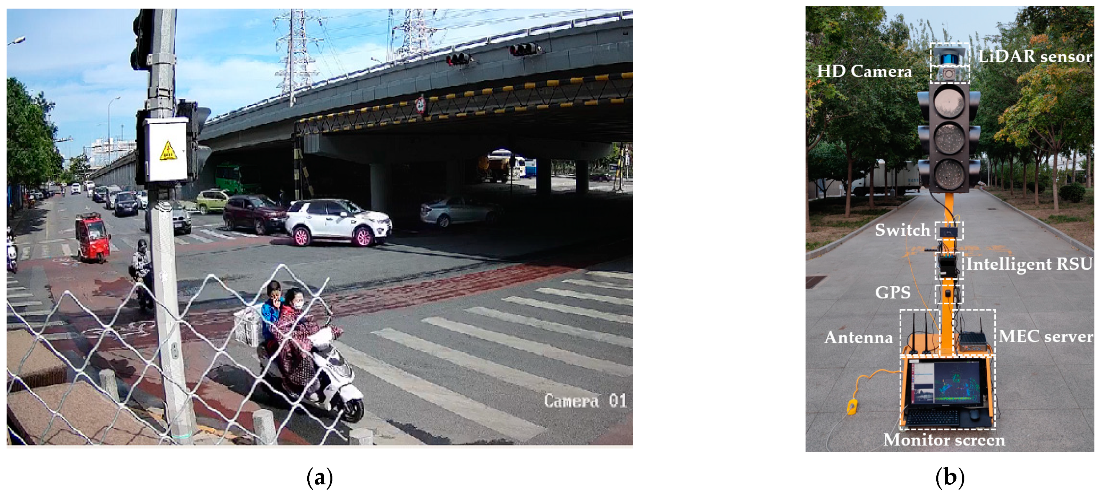
3.1. Field Test and Data Analysis

In the field test, a typical intersection, located in Fushi Road, Shijingshan District, Beijing City, is selected as the experimental intersection. There are four lanes in one direction from east to west, and the rightmost lane is the dedicated right-turn lane, which is not controlled by traffic lights, as shown in Figure 9a. In addition, we design a mobile intelligent roadside perception and computing platform for multiple test scenarios. The intelligent roadside platform consists of the LiDAR sensor, HD camera, switch, intelligent RSU, GPS, MEC server and monitor screen, as shown in Figure 9b.

At the experimental platform, the resolution of the camera is 1080 P (1920 × 1080) with a sampling rate of 25 Hz. After testing, the resolution can detect and recognize targets about 200 m. The LiDAR sensors with 32 lines can detect surrounding environment about 300 m. The camera is responsible for detecting traffic signs and vehicles, while the LiDAR sensor is for exploring blind spots and long-distance targets in complex traffic environment.

In the experiment, we intercepted test data in 30 min, which is collected by the roadside perception platform containing a series of vehicles, pedestrians, and buildings. After data preprocessing, about 22,000 pieces of vehicular data are obtained, which are shown in

Table 2. Dataset of vehicles.

V2X Communication	License Plate	Latitude	Longitude	Rev (r/s)	Steering Angle (°)	Speed (m/s)	Acceleration (m/s2)	Horizontal Distance (m)	Heading Angle (°)
Yes	N C5530	116.201054	39.923663	0.05	15	0.10	−0.06	5.82	7.30
No	N 46735	116.200968	39.923662	——	——	1.26	——	11.71	6.52
︙	︙	︙	︙	︙	︙	︙	︙	︙	︙
Yes	A V3210	116.2011	39.923624	2.4	43	4.32	0.33	20.15	13.49
No	U B3957	116.201055	39.9236244	——	——	4.98	——	12.43	8.03

and

Table 3. Dataset of the traffic state.

Time Stamp	Traffic Flow (veh/s)	Average Speed (m/s)	Average Queue Length(m)	Signal Cycle (s)	Signal Light (E→W)	Signal Remaining Time (s)
1609232611	5	1.38	6.80	105	Red	10
1609232612	7	0.83	14.80	105	Red	9
︙	︙	︙	︙	︙	︙	︙
1609234429	13	3.44	0	105	Green	5
1609234430	11	2.85	0	105	Green	4

.

3.2. Evaluation Index

To describe the performance of the GCN–GRU model, the following three indexes are proposed to evaluate the predicted results.

(1)

Root mean squared error (RMSE)

$$RMSE=\sqrt{\frac{{\displaystyle {\sum }_{t=1}^m{(y_t-{\widehat{y}}_t)}^2}}{m}}$$

(16)

(2)

Mean absolute error (MAE)

$$MAE=\frac{{\displaystyle {\sum }_{i=1}^m|y_t-{\widehat{y}}_t|}}{m}$$

(17)

(3)

Accuracy (Accuracy)

$$Accuracy=1-\frac{{\Vert y_t-{\widehat{y}}_t\Vert }_F}{{\Vert y_t\Vert }_F}$$

(18)

where $y_t$ and ${\widehat{y}}_t$ represent the real traffic state value and predicted traffic state value, respectively.

RMSE and MAE can reflect the difference between the real value and the predicted value, and both two values fall into the interval [0, +∞). These evaluation values are negatively correlated with the prediction effect, that is, the smaller the value is, the better the prediction effect is. Accuracy is used to detect the precision of predicted results, that is, the larger the value is, the better the prediction effect is.

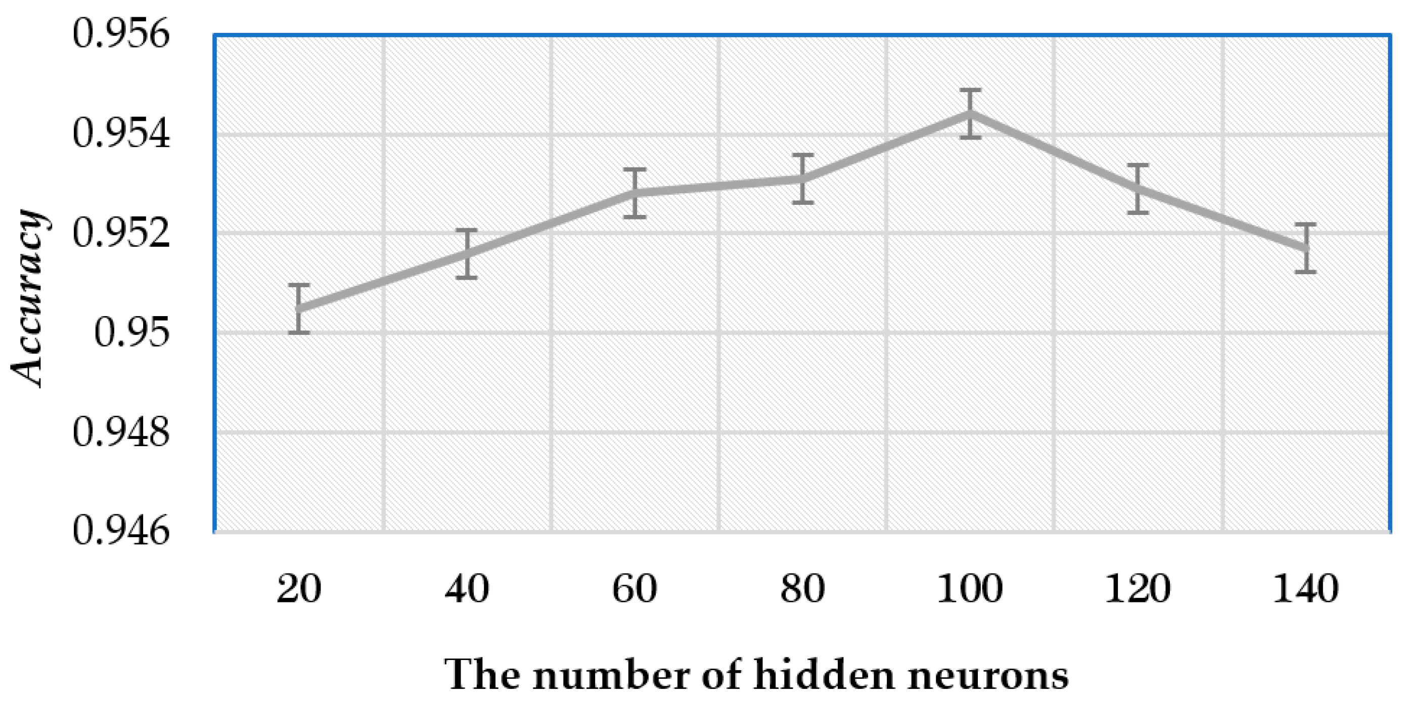
3.3. Parameter Settings

In the experiment, we normalize the traffic data to the interval [0, 1] and the purpose is to speed up model training. In addition, we treat 70% of the dataset as the training set and the remaining 30% as the test set. In this experiment, the learning rate of the model is 0.001, the size of batch is 32 and the size of epoch is 800. In addition, the model uses L2 regularization to prevent over-fitting. Adam optimizer with gradient descent is employed to train the model.

In the multi-source information fusion of the dataset based on V2X technology, we set the size of the hidden layer to 20, 40, 60, 80, 100, 120, and 140, respectively.

Table 4. The predicted errors in different hidden neurons.

The Number of Hidden Neurons	RMSE	MAE	Accuracy
20	2.8942	1.9852	0.9505
40	2.7863	1.9723	0.9516
60	2.7021	1.9623	0.9528
80	2.6967	1.9483	0.9531
100	2.6547	1.9372	0.9544
120	2.7654	1.9521	0.9529
140	2.7735	1.9652	0.9517

shows the comparison of prediction performance under different hidden neurons. Figure 10 shows the comparison of prediction accuracy under different hidden neurons in the dataset. It can be seen from the results that the over-fitting phenomenon occurs when the number of neural units in the hidden layer increases from 20 to 140, the prediction accuracy increases at first and then decreases. When the number of neurons in the hidden layer is 100, the Accuracy is 0.9544. Therefore, the number of hidden layer neurons set in the model is set to 80.

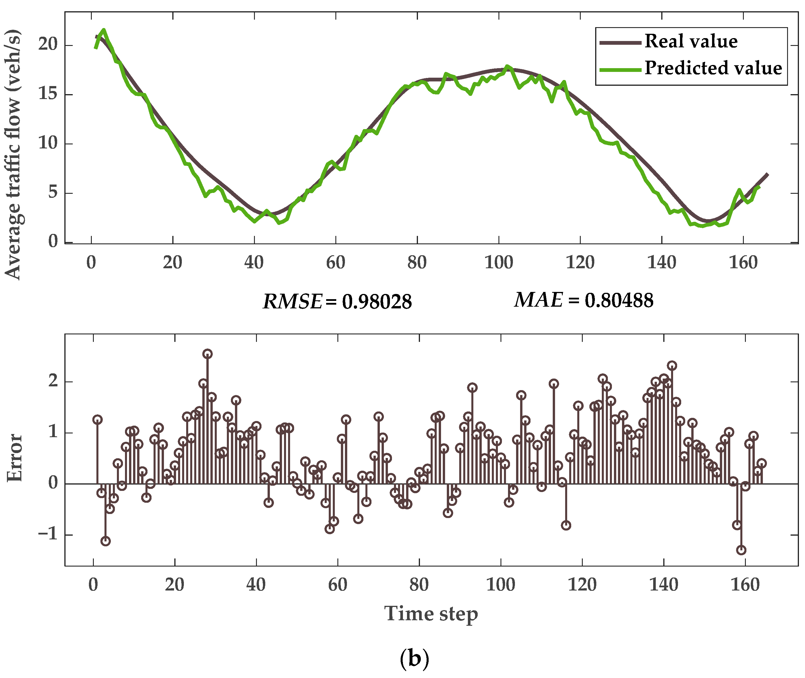
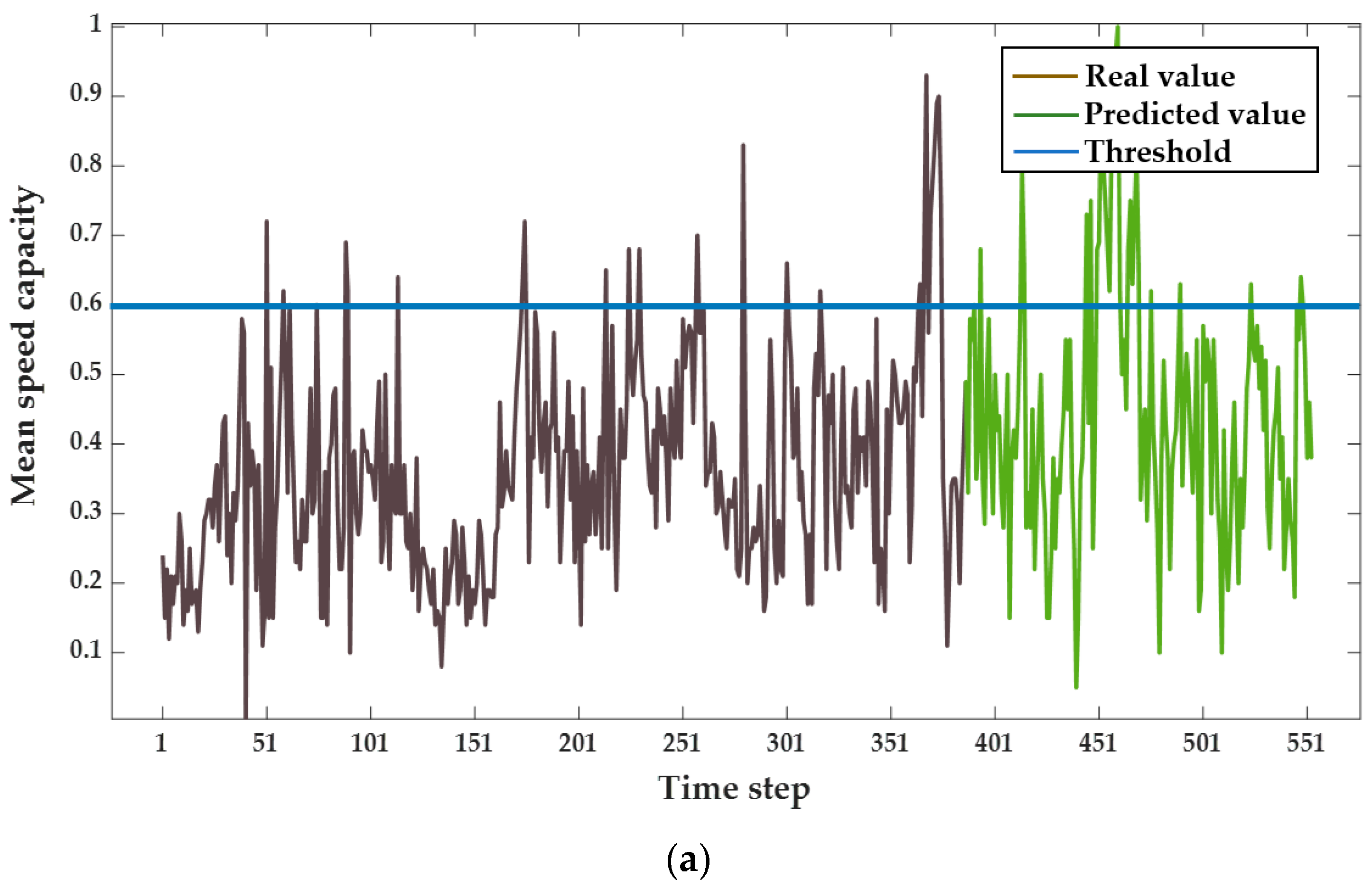
3.4. Performance of Prediction Model

Based on the perception dataset of the traffic state, the experiment predicts the average traffic flow and the mean speed capacity of urban intersections in a short term. The specific analyses are presented as follows.

Figure 11a shows the performance of the training model with dividing the dataset of the average traffic flow by 7:3 for training and testing. Figure 11b shows the fitting results of the actual average traffic flow data and the predicted results, as well as the errors between the predicted values and the real observed values. It is worth noting that the average traffic flow of the intersection has spatiotemporal periodicity, and the model accurately predicts the trend at the next time step by learning the spatiotemporal correlation of data. The values of RMSE and MAE are 0.9823 and 0.8049, respectively, which prove that the prediction results can meet the requirements [32,33].

Figure 12a shows the performance of the training model with dividing the dataset of the mean speed capacity by 7:3 for training and testing. For the threshold is set up as 0.6, the time of the mean speed capacity exceeding the threshold can be observed obviously. The prediction results can be treated as a reference to evaluate the short-term traffic state of the intersection in real time.

As shown in Figure 12b, the fitting results between the real observation valued and the predicted valued of the mean speed capacity meets the predicted requirements [34]. The values of RMSE and MAE are 0.1970 and 0.1585, respectively, which can prove that the prediction model is effective.

Through the prediction of the average traffic flow and mean speed capacity, the traffic operation state of intersections can be perceived in real time. At the same time, it can provide data support for traffic managers to conduct real-time traffic guidance at intersections and relieve the queuing pressure at intersections.

In order to validate effectiveness of the proposed model, we compare it with the other four predicted models, including LSTM, RNN, CNN, and back propagation (BP) neural network models. In the process of prediction, we choose the same parameters described in Section 3.3.

Table 5. Comparison results of the average traffic flow.

Time	Evaluation Index	GCN–GRU	LSTM	RNN	CNN	BP
5 min	MAE	1.0002	1.9823	3.5521	4.3511	3.8552
	RMSE	1.2354	2.9940	5.3215	6.5362	4.5113
	Accuracy	0.949	0.832	0.775	0.682	0.751
10 min	MAE	0.9303	1.9823	3.3241	4.3012	3.8463
	RMSE	1.1532	2.9940	4.9215	6.4621	4.4963
	Accuracy	0.954	0.832	0.779	0.682	0.758
15 min	MAE	0.8049	1.9838	3.4843	4.2984	3.8466
	RMSE	0.9803	2.9843	5.0122	6.4551	4.4985
	Accuracy	0.958	0.845	0.780	0.671	0.756
30 min	MAE	0.7842	1.8856	3.5012	4.3123	3.8512
	RMSE	0.9053	2.7650	5.1230	6.5010	4.5013
	Accuracy	0.967	0.883	0.789	0.663	0.758

and

Table 6. Comparison results of the mean speed capacity.

Time	Evaluation Index	GCN–GRU	LSTM	RNN	CNN	BP
5 min	MAE	0.2911	0.5451	0.9528	1.4213	0.9984
	RMSE	0.2935	0.6654	1.0981	1.7520	1.2135
	Accuracy	0.965	0.852	0.781	0.625	0.773
10 min	MAE	0.2133	0.5431	0.9413	1.5312	0.9988
	RMSE	0.2465	0.6641	1.0005	1.7640	1.2141
	Accuracy	0.967	0.864	0.788	0.631	0.771
15 min	MAE	0.1835	0.5394	0.9641	1.4812	0.9985
	RMSE	0.2004	0.6604	1.2154	1.7024	1.2031
	Accuracy	0.966	0.865	0.791	0.640	0.773
30 min	MAE	0.1585	0.5388	0.9721	1.5531	0.9971
	RMSE	0.1970	0.6541	1.3412	1.7233	1.1998
	Accuracy	0.965	0.859	0.799	0.627	0.772

show comparison results of the average traffic flow and mean speed capacity for 5, 10, 15, and 30 min, respectively.

In addition, the experiments also compare the training time and prediction time between the GCN–GRU model and the other four models, as shown in

Table 7. The computational cost of LSTM, RNN, CNN, BP, and GCN–GRU.

	LSTM	RNN	CNN	BP	GCN–GRU
Training time	183.2 s	105.4 s	309.7 s	123.4 s	112.3 s
Prediction time	1.353 s	0.932 s	2.332 s	1.234 s	0.995 s

.

It can be seen from Table 7 that the training time and prediction time of GCN–GRU model are longer than that with the RNN model. However, the prediction accuracy of GCN–GRU model is much higher than that in other models. We can infer that the proposed method is practical and significant in the objective of improving the predicted accuracy. To sum up, the prediction performances of GCN–GRU are better than that with other neural network prediction models in prediction accuracy.

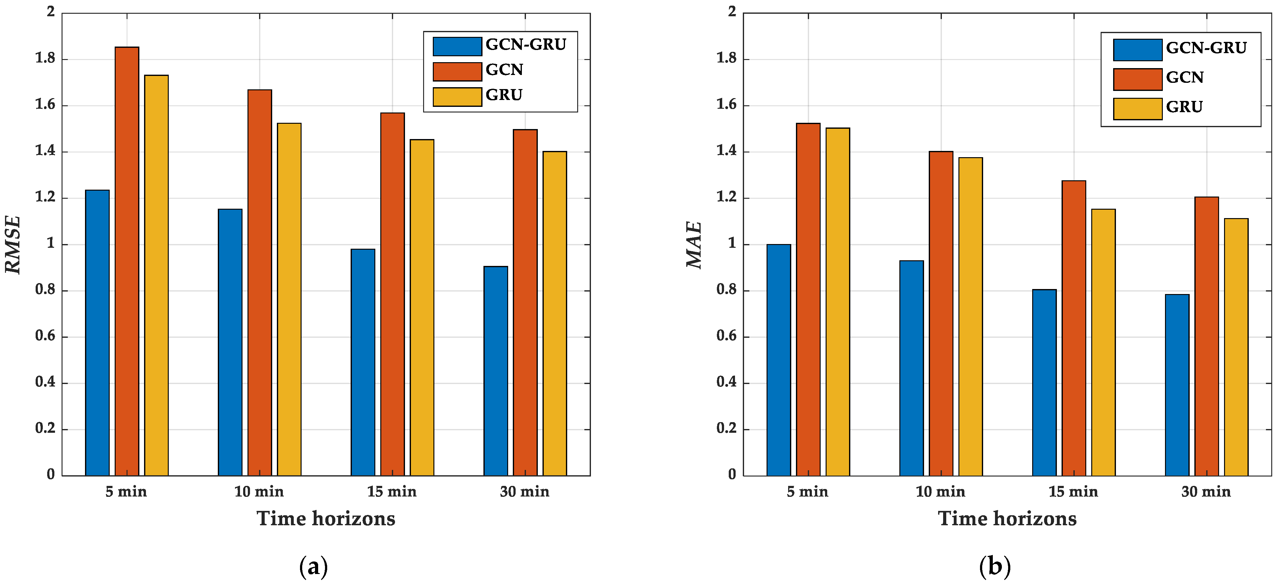
3.5. Comparison Experiment Results

To verify whether the proposed model can effectively extract the spatiotemporal features from the dataset of traffic state, we compare the GCN–GRU model with GRU and GCN model in the experiment. As shown in Figure 13 and Figure 14, the average traffic flow and the mean speed capacity at the time points 5, 10, 15, and 30-min are compared, respectively, and then the error performances are analyzed intensively.

In the beginning 5 min, by comparing with the GCN model which only considers spatial features, the predictions for the average traffic flow, the RMSE and MAE show the superiority of our proposed GCN–GRU model with 33.35% and 34.4% reductions. In the same way, for the 10, 15, and 30-min prediction of the average traffic flow, the RMSE performed in our GCN–GRU model is reduced by 30.89%, 37.51% and 39.53%, respectively, and the MAE is reduced by 33.66%, 36.9% and 34.95%, respectively. Thus, it can be clearly observed that RMSE and MAE errors of the proposed model have been significantly reduced. We infer that our proposed GCN–GRU model can extract spatial features efficiently.

Similarly, by comparing the prediction results of our GCN–GRU model with the GRU model at the time points 5, 10, 15 and 30 min, the RMSE of the GCN–GRU model is reduced by 28.68%, 24.36%, 32.54% and 35.43%, and the MAE is reduced by 33.47%, 32.39%, 30.2%, and 29.5%, respectively. The prediction results indicate that the GCN–GRU model can also efficiently extract temporal features.

In Figure 14, the predicted performance of the GCN–GRU model is consistent with the average traffic flow in the mean speed capacity. The errors of RMSE and MAE are reduced to a certain extent, then remain relatively stable in (0.2, 0.3) and (0.1, 0.3), respectively. Therefore, the significant error reductions of the proposed GCN–GRU in EMSE and MAE reveal that fusing the spatiotemporal features is effective in accurate short-term traffic flow prediction.

4. Conclusions

To improve the traffic efficiency, we proposed a short-term traffic state prediction model based on the data acquisition strategy of MEC-assisted V2X network. The model combines the advantages of GCN and GRU soft-attention mechanism to analyze the spatiotemporal characteristics of traffic data. In addition, we design an intelligent roadside platform to verify the proposed model. The main conclusions are summarized as follows:

(1)

This paper fuses multi-source information between intelligent OBUs, roadside sensors and traffic signal controller to accurately perceive the traffic state based on the V2X communication.

(2)

The prediction model considers the spatiotemporal dependence of all vehicles at vertexes of the intersection network. The proposed model can effectively extract vertexes features from the intersection, which greatly improves the prediction accuracy of the model. Based on the data acquisition strategy of the MEC-assisted V2X network, the comparative experiment reveals the effectiveness of our proposed model.

(3)

This paper mainly analyzes the traffic operation state of the single intersection, which limits the usage of the proposed model in extended scenarios and may pose a challenge to the adaptability of the model. In further research, we will study the traffic state prediction problems with the regional intersections to explore the efficiency and effectiveness of data support and implementation scheme in CVIS, as well as the adaptability of the model in these scenarios.

References

1. Su, X.; Fan, M.; Zhang, M.; Liang, Y. An innovative approach for the short-term traffic flow prediction. J. Syst. Sci. Syst. Eng. 2021, 30, 519–532. [Google Scholar] [CrossRef]
2. Salamanis, A.; Margaritis, G.; Kehagias, D.D.; Matzoulas, G.; Tzovaras, D. Identifying patterns under both normal and abnormal traffic conditions for short-term traffic prediction. Transp. Res. Proc. 2017, 22, 665–674. [Google Scholar] [CrossRef]
3. He, Z.; Chow, C.; Zhang, J. STCNN: A Spatio-temporal convolutional neural network for long-term traffic prediction. In Proceedings of the 2019 20th IEEE International Conference on MDM, Hong Kong, China, 10–13 June 2019; pp. 226–233. [Google Scholar] [CrossRef]
4. Schakel, W.J.; Van Arem, B. Improving traffic flow efficiency by in-car advice on lane, speed, and headway. In Proceedings of the Transportation Research Board 92nd Annual Meeting Compendium of Papers, Washington, DC, USA, 13–17 January 2013. [Google Scholar] [CrossRef]
5. Ma, J.; Han, W.; Guo, Q.; Zhang, S. Enhancing traffic capacity of scale-free networks by link-directed strategy. Int. J. Mod. Phys. C 2016, 27, 1650028. [Google Scholar] [CrossRef]
6. Ghiasi, A.; Hussain, O.; Qian, Z.; Li, X. A mixed traffic capacity analysis and lane management model for connected automated vehicles: A Markov chain method. Transp. Res. B-Meth. 2017, 106, 266–292. [Google Scholar] [CrossRef]
7. Wang, X.; Han, J.; Bai, C.; Shi, H.; Zhang, J.; Wang, G. Research on the impacts of generalized preceding vehicle information on traffic flow in V2X environment. Fut. Int. 2021, 13, 88. [Google Scholar] [CrossRef]
8. Wang, P.; Jiang, Y.; Xiao, L.; Zhao, Y.; Li, Y. A joint control model for connected vehicle platoon and arterial signal coordination. J. Intell. Transp. Syst. 2020, 24, 81–92. [Google Scholar] [CrossRef]
9. Yan, J.; Li, H.; Bai, Y.; Lin, Y. Spatial-temporal traffic flow data restoration and prediction method based on the tensor decomposition. Appl. Sci. 2021, 11, 9220. [Google Scholar] [CrossRef]
10. Wang, C.; Ran, B.; Yang, H.; Zhang, J.; Qu, X. A novel approach to estimate freeway traffic state: Parallel computing and improved kalman filter. IEEE Intell. Transp. Syst. Mag. 2018, 10, 180–193. [Google Scholar] [CrossRef]
11. Zhang, Y.; Wang, S.; Chen, B.; Cao, J.; Huang, Z. TrafficGAN: Network-scale deep traffic prediction with generative adversarial nets. IEEE Trans. Intell. Transp. Syst. 2019, 22, 219–230. [Google Scholar] [CrossRef]
12. Lv, Y.; Duan, Y.; Kang, W.; Li, Z.; Wang, F. Traffic flow prediction with big data: A deep learning approach. IEEE Trans. Intell. Transp. Syst. 2015, 16, 865–873. [Google Scholar] [CrossRef]
13. Li, Y.; Yu, R.; Shahabi, C.; Liu, Y. Diffusion convolutional recurrent neural network: Data-driven traffic forecasting. arXiv 2018, arXiv:1707.01926. [Google Scholar]
14. Nguyen, H.; Le, M.K.; Tao, W.; Chen, C. Deep learning methods in transportation domain: A review. IET Intel. Transp. Syst. 2018, 12, 998–1004. [Google Scholar] [CrossRef]
15. Fang, W.; Zhong, B.; Zhao, N.; Love, E.D.P.; Luo, H.; Xue, J.; Xu, S. A deep learning-based approach for mitigating falls from height with computer vision: Convolutional neural network. Adv. Eng. Inf. 2019, 39, 170–177. [Google Scholar] [CrossRef]
16. Yin, W.; Kann, K.; Yu, M.; Sch, H. Comparative study of CNN and RNN for natural language processing. arXiv 2017, arXiv:1702.01923. [Google Scholar]
17. Liu, Y.; Gong, C.; Yang, L.; Chen, Y. DSTP-RNN: A dual-stage two-phase attention-based recurrent neural network for long-term and multivariate time series prediction. Exp. Syst. Appl. 2020, 143, 113082. [Google Scholar] [CrossRef]
18. Yuan, Y.; Shao, C.; Cao, Z.; He, Z.; Zhu, C.; Wang, Y.; Jang, V. Bus dynamic travel time prediction: Using a deep feature extraction framework based on RNN and DNN. Electronics 2020, 9, 1876. [Google Scholar] [CrossRef]
19. Zeng, Y.; Shao, M.; Sun, L.; Lu, C. Traffic prediction and congestion control based on directed graph convolution neural network. China J. Highw. Transp. 2021, 5, 1–16. [Google Scholar]
20. Cui, Z.; Henrickson, K.; Ke, R.; Wang, Y.H. Traffic graph convolutional recurrent neural network: A deep learning framework for network-scale traffic learning and forecasting. IEEE Trans. Intell. Transp. Syst. 2019, 21, 4883–4894. [Google Scholar] [CrossRef] [Green Version]
21. Ye, J.; Sun, L.; Du, B.; Fu, Y.; Xiong, H. Coupled layer-wise graph convolution for transportation demand prediction. arXiv 2020, arXiv:2012.08080. [Google Scholar]
22. Ma, X.; Dai, Z.; He, Z.; Na, J.; Wang, Y.; Wang, Y. Learning traffic as images: A deep convolutional neural network for large-scale transportation network speed prediction. Sensors 2017, 17, 818. [Google Scholar] [CrossRef] [Green Version]
23. Li, Z.; Xiong, G.; Tian, Y.; Lv, Y.; Chen, Y.; Hui, P.; Su, X. A multi-stream feature fusion approach for traffic prediction. IEEE Trans. Intell. Transp. Syst. 2020, 1–11. [Google Scholar] [CrossRef]
24. Wang, P.; Deng, H.; Zhang, J.; Wang, L.; Zhang, M.; Li, Y. Model predictive control for connected vehicle platoon under switching communication topology. IEEE Trans. Intell. Transp. Syst. 2021. [Google Scholar] [CrossRef]
25. Giovanni, B.; YannAel, L.B.; Gianluca, B.; Karl, D. On-board-unit data: A big data platform for scalable storage and processing. In Proceedings of the 2018 4th International Conference on CloudTech, Brussels, Belgium, 26–28 November 2018; pp. 1–5. [Google Scholar] [CrossRef]
26. Mondal, S.; Gupta, A. Assessment of saturation flow at signalized intersections: A synthesis of global perspective and future directions. Curr. Sci. 2020, 119, 32–43. [Google Scholar] [CrossRef]
27. Ma, X.; Miao, R.; Wu, X.; Liu, X. Examining influential factors on the energy consumption of electric and diesel buses: A data-driven analysis of large-scale public transit network in Beijing. Energy 2021, 216, 119196. [Google Scholar] [CrossRef]
28. Wang, P.; Wang, Y.; Deng, H.; Zhang, M.; Zhang, J. Multilane spatiotemporal trajectory optimization method (MSTTOM) for connected vehicles. J. Adv. Transp. 2020. [Google Scholar] [CrossRef]
29. Liu, X.; Qu, X.; Ma, X. Improving flex-route transit services with modular autonomous vehicles. Transport. Res. E-Log. 2021, 149, 1366–5545. [Google Scholar] [CrossRef]
30. Minh, Q.T.; Kamioka, E. Traffic state estimation with mobile phones based on the “3R” philosophy. IEEE Trans. Commun. 2011, 12, 3447–3458. [Google Scholar] [CrossRef]
31. Yang, S.; Su, Y.; Chang, Y.; Hung, H. Short-term traffic prediction for edge computing-enhanced autonomous and connected cars. IEEE Trans. Veh. Techn. 2019, 68, 3140–3153. [Google Scholar] [CrossRef]
32. Gu, Y.; Xu, X.; Qin, L.; Shao, Z.; Zhang, H. An improved Bayesian combination model for short-term traffic prediction with deep learning. IEEE Trans. Intell. Transp. Syst. 2020, 21, 1924–9050. [Google Scholar] [CrossRef]
33. Liu, X.; Qu, X.; Ma, X. Optimizing electric bus charging infrastructure considering power matching and seasonality. Transport. Res. D-Trans. 2021, 100, 1361–9209. [Google Scholar] [CrossRef]
34. Andreas, R.; Felix, K.; Ralph, R.; Klaus, D. Car2x-based perception in a high-level fusion architecture for cooperative perception systems. In Proceedings of the 2012 IEEE Intelligent Vehicles Symposium, Madrid, Spain, 3–7 June 2012; pp. 270–275. [Google Scholar] [CrossRef]
Figure 1. The framework of the proposed method.
Applsci 11 11530 g001
Figure 2. Traffic perception system based on V2X communication.
Applsci 11 11530 g002
Figure 3. MEC architecture.
Applsci 11 11530 g003
Figure 4. The data processing progress of the MEC paradigm.
Applsci 11 11530 g004
Figure 5. The prediction model network.
Applsci 11 11530 g005
Figure 6. Graphs of vehicular state at intersection.
Applsci 11 11530 g006
Figure 7. The structure of GRU unit.
Applsci 11 11530 g007
Figure 8. The structure of the soft-attention mechanism.
Applsci 11 11530 g008
Figure 9. Experimental field. (a) Experimental intersection; (b) Experimental platform.
Applsci 11 11530 g009
Figure 10. The comparison of prediction Accuracy under different hidden neurons.
Applsci 11 11530 g010
Figure 11. Prediction results of the average traffic flow. (a) The training performance of real value and predicted value in average traffic flow; (b) Fitting results of the actual average traffic flow data and the predicted results; errors between the predicted values and the real observed values.
Applsci 11 11530 g011aApplsci 11 11530 g011b
Figure 12. Prediction results of the mean speed capacity. (a) The training performance of real value and predicted value in mean speed capacity; (b) Fitting results between the real value and the predicted value of the mean speed capacity; errors between the predicted values and the real observed values.
Applsci 11 11530 g012aApplsci 11 11530 g012b
Figure 13. Comparison results of the average traffic flow prediction. (a) The comparative experiment of the RMSE; (b) The comparative experiment of the MAE.
Applsci 11 11530 g013
Figure 14. Comparison results of the mean speed capacity. (a) The comparative experiment of the RMSE; (b) The comparative experiment of the MAE.
Applsci 11 11530 g014