
A Fusion of Feature-Oriented Principal Components of Multispectral Data to Map Granite Exposures of Pakistan

 ,
,  ,
,  ,
,  ,
, 
Abstract
1. Introduction
2. Geology of Shewa Shahbazghari and Ambela Granite Complexes
3. Materials and Methods
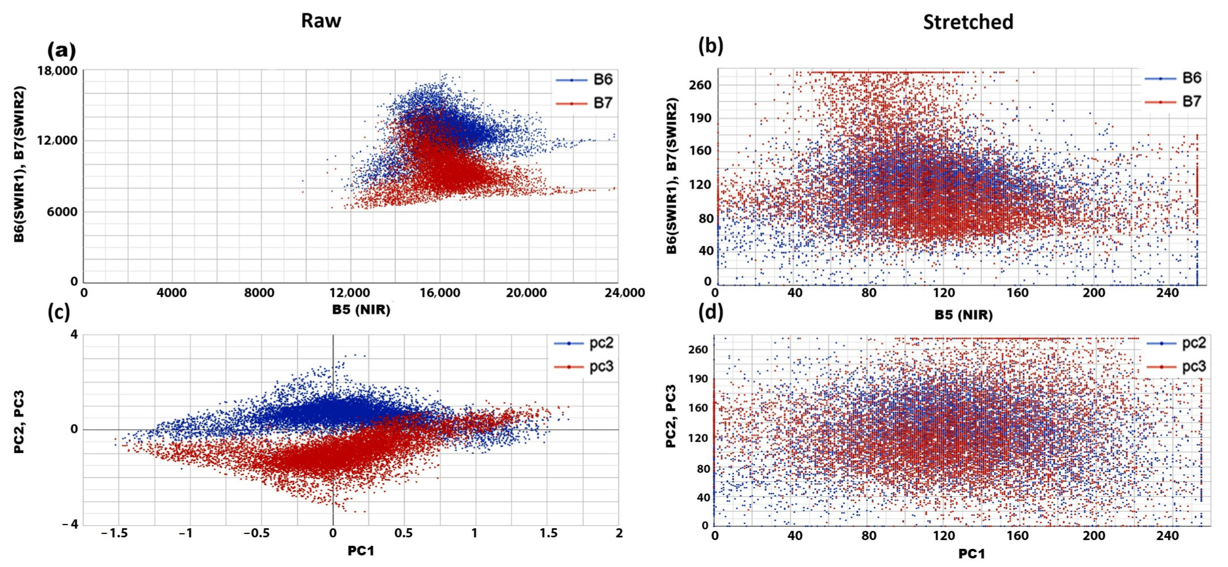
3.1. PCA
3.2. DS
3.3. Mapping in Dense Vegetation by the Fusion of FPCS Components from Different Data Sources Using GEE
3.3.1. Pre-Processing and Selection of Suitable Multispectral Bands
3.3.2. Application of PCA
3.3.3. Fusion of the Selected Crosta Components
4. Results
4.1. FPCS of the Landsat-8 Data
4.2. FPCS of the ASTER Data
4.3. FPCS of the Sentinel-2 MSI Data
4.4. The Fusion of the Selected Sentinel-2 MSI and Landsat-8 Components
5. Discussion
6. Conclusions
- A time-efficient methodology for fusing selective FPCS components from stretched and raw Landsat-8 OLI + Landsat-8 TIRS, ASTER, and Sentinel-2 MSI is presented to map granite and marble of Shewa Shahbazghari area. The process took 147.14 s on the GEE Cloud computing platform to carry out PCA in three multispectral data sources’ raw and stretched forms.
- A weighted linear combination of PCs was carried out based on each component’s granite and marble indicating features to enhance granitic spectral features while suppressing others. The results were validated by matching all the exposed granite and marble quarries successfully.
- The TIR bands of the ASTER had a 90 m resolution that did not perform well in densely vegetated areas; therefore, a combination of Landsat-8 and Sentinel-2 components discriminated the granite/marble rock types better in Shewa Shahbazgarhi due to much better resolutions. Furthermore, the non-availability of granite absorption features from the TIR bands in Sentinel-2 MSI datasets was overcome by Landsat-8 TIR bands. As a result, the high-resolution SWIR bands from Sentinel-2 and the medium-to-low-resolution TIR bands from Landsat-8 TIRS helped obtain the final FCC map for discriminating granite from marble.
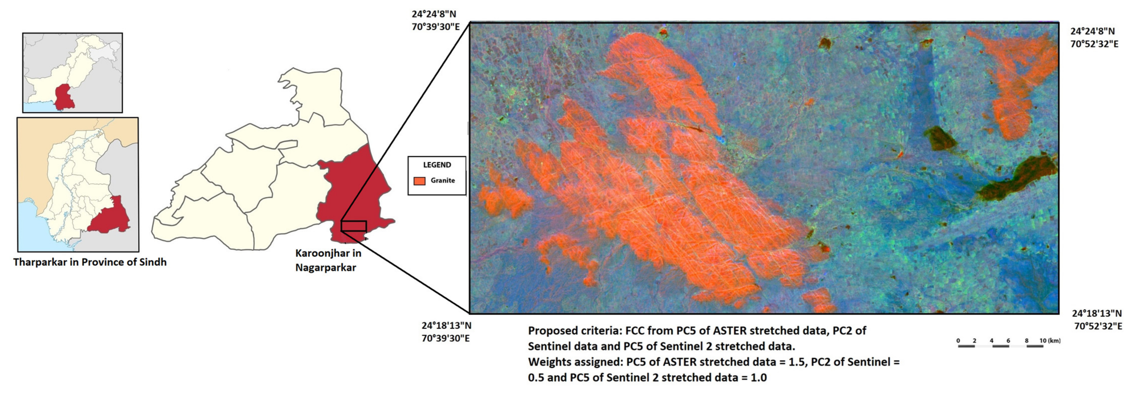
- The weighted PCs extrapolation to other granite outcrops across Pakistan showed the technique’s usefulness to obtain results with ease and accuracy. In less vegetated regions, i.e., the Kotah Dome, Malakand, and non-vegetated Karoonjhar Nagarparkar, the ASTER component was helpful due to the granite-specific TIR2 band. The advantage of Sentinel-2 components was highlighted in all case studies, which shows that high-spatial-resolution SWIR bands support TIR bands from the ASTER and/or Landsat in mapping granite and accessory minerals. The information about accessory granite minerals due to their spectral absorption in the SWIR2 band is incorporated in granite through the high-spatial-resolution Sentinel-2 components bearing high-resolution SWIR2 bands.
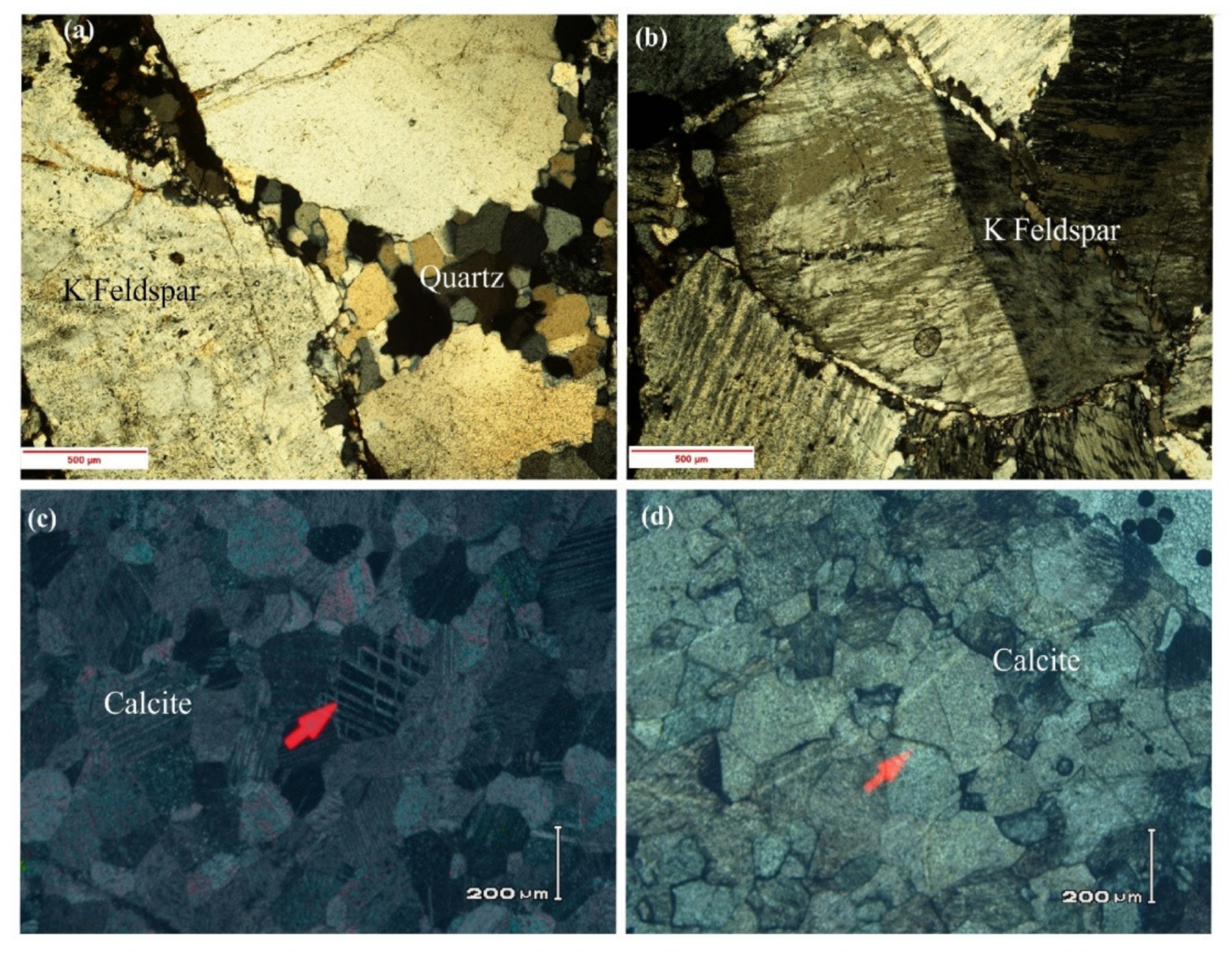
- Based on the analysis of eigenvector loadings, the low emissivity in Landsat-8 TIR1 and the reflection of the SWIR1 (1570 nm–1660 nm) and SWIR2 (2110 nm–2290 nm) bands were observed due to orthoclase and quartz in granite. The SWIR2 components from Landsat-8 and Sentinel-2 indicated absorption characteristics of granite accessory minerals, i.e., muscovite, epidote, and amphibole. Similarly, marble showed absorption features in the SWIR2 (2110–2290 nm) band of Landsat-8 OLI and Sentinel-2.
- The methodology can be further used for high-end RS applications:
- a.
- Predicting geotechnical properties through mineralogy using freely available multispectral or commercial high-resolution datasets (Worldview3, Quick bird, Spot Eye, etc.).
- b.
- Unsupervised classification for better data annotation before using machine learning/deep learning algorithms.
Author Contributions
Funding
Institutional Review Board Statement
Informed Consent Statement
Acknowledgments
Conflicts of Interest
References
- Bermúdez-Lugo, O. The Mineral Industry of Ghana; USGS Minerals Yearbook. 2011. Available online: https://bit.ly/3r9Eltx (accessed on 12 September 2021).
- Van der Meer, F.D.; van der Werff, H.M.A.; van Ruitenbeek, F.J.A.; Hecker, C.A.; Bakker, W.H.; Noomen, M.F.; van der Meijde, M.; Carranza, E.J.M.; Smeth, J.B.; de Woldai, T. Multi—and hyperspectral geologic remote sensing: A review. Int. J. Appl. Earth Obs. Geoinf. 2012, 14, 112–128. [Google Scholar] [CrossRef]
- Hirai, A. Mineral discrimination by combination of multispectral image and surrounding hyperspectral image. J. Appl. Remote Sens. 2019, 13, 1. [Google Scholar] [CrossRef]
- Gupta, R.P. Remote Sensing Geology, 2nd ed.; Springer: Berlin/Heidelberg, Germany, 2003; ISBN 978-3-642-07741-8. [Google Scholar]
- LP DAAC—Change in Status Alert for the ASTER SWIR Detector. Available online: https://lpdaac.usgs.gov/news/change-status-alert-aster-swir-detector/ (accessed on 10 December 2020).
- Suhet, H.B. Sentinel-2 User Handbook 2015; European Space Agency (ESA). Available online: https://sentinel.esa.int/documents/247904/685211/Sentinel-2_User_Handbook (accessed on 11 August 2021).
- Van der Werff, H.; van der Meer, F. Sentinel-2A MSI and Landsat 8 OLI Provide Data Continuity for Geological Remote Sensing. Remote Sens. 2016, 8, 883. [Google Scholar] [CrossRef]
- Adiri, Z.; Lhissou, R.; El Harti, A.; Jellouli, A.; Chakouri, M. Recent advances in the use of public domain satellite imagery for mineral exploration: A review of Landsat-8 and Sentinel-2 applications. Ore Geol. Rev. 2020, 117, 103332. [Google Scholar] [CrossRef]
- Madani, A.A.; Emam, A.A. SWIR ASTER band ratios for lithological mapping and mineral exploration: A case study from El Hudi area, southeastern desert, Egypt. Arab. J. Geosci. 2011, 4, 45–52. [Google Scholar] [CrossRef]
- Mars, J.C.; Rowan, L.C. Spectral assessment of new ASTER SWIR surface reflectance data products for spectroscopic mapping of rocks and minerals. Remote Sens. Environ. 2010, 114, 2011–2025. [Google Scholar] [CrossRef]
- Neinavaz, E.; Schlerf, M.; Darvishzadeh, R.; Gerhards, M.; Skidmore, A.K. Thermal infrared remote sensing of vegetation: Current status and perspectives. Int. J. Appl. Earth Obs. Geoinf. 2021, 102, 102415. [Google Scholar] [CrossRef]
- Traore, M.; Çan, T.; Tekin, S. Discrimination of Iron Deposits Using Feature Oriented Principal Component Selection and Band Ratio Methods: Eastern Taurus /Turkey. Int. J. Environ. Geoinform. 2020, 7, 147–156. [Google Scholar] [CrossRef]
- Yamaguchi, Y.; Naito, C. Spectral indices for lithologic discrimination and mapping by using the ASTER SWIR bands. Int. J. Remote Sens. 2003, 24, 4311–4323. [Google Scholar] [CrossRef]
- Huang, S.; Chen, S.B.; Zhang, Y.Z. Comparison of altered mineral information extracted from ETM+, ASTER and Hyperion data in Águas Claras iron ore, Brazil. IET Image Process. 2019, 13, 355–364. [Google Scholar] [CrossRef]
- Asadzadeh, S.; de Souza Filho, C.R. A review on spectral processing methods for geological remote sensing. Int. J. Appl. Earth Obs. Geoinf. 2016, 47, 69–90. [Google Scholar] [CrossRef]
- Abdelmalik, K.W. Landsat 8: Utilizing sensitive response bands concept for image processing and mapping of basalts. Egypt. J. Remote Sens. Sp. Sci. 2019, 23, 263–274. [Google Scholar] [CrossRef]
- Khan, A.; Faisal, S.; Shafique, M.; Khan, S.; Bacha, A.S. ASTER-based remote sensing investigation of gypsum in the Kohat Plateau, north Pakistan. Carbonate. Evaporite 2020, 35, 1–13. [Google Scholar] [CrossRef]
- Askari, G.; Pour, A.B.; Pradhan, B.; Sarfi, M.; Nazemnejad, F. Band ratios matrix transformation (BRMT): A sedimentary lithology mapping approach using ASTER satellite sensor. Sensors 2018, 18, 3213. [Google Scholar] [CrossRef]
- Moradi, M.; Basiri, S.; Kananian, A.; Kabiri, K. Fuzzy logic modeling for hydrothermal gold mineralization mapping using geochemical, geological, ASTER imageries and other geo-data, a case study in Central Alborz, Iran. Earth Sci. Inform. 2015, 8, 197–205. [Google Scholar] [CrossRef]
- Eslami, A.; Ghaderi, M.; Rajendran, S.; Pour, A.B.; Hashim, M. Integration of ASTER and landsat TM remote sensing data for chromite prospecting and lithological mapping in Neyriz ophiolite zone, south Iran. Resour. Geol. 2015, 65, 375–388. [Google Scholar] [CrossRef]
- Pournamdari, M.; Hashim, M. Detection of chromite bearing mineralized zones in Abdasht ophiolite complex using ASTER and ETM+ remote sensing data. Arab. J. Geosci. 2014, 7, 1973–1983. [Google Scholar] [CrossRef]
- Martinez-Izquierdo, M.E.; Molina-Sanchez, I.; Morillo-Balsera, M.D.C. Efficient Dimensionality Reduction using Principal Component Analysis for Image Change Detection. IEEE Lat. Am. Trans. 2019, 17, 540–547. [Google Scholar] [CrossRef]
- Negrón, L.M.; Piranian, M.; Amaya, M.A.; Gorski, D.; Pingitore, N.E. ArcGISTMand Principal Component Analysis of Probe Data to Micro-Map Minerals in Round Top Rare Earth Deposit. Adv. Mater. Phys. Chem. 2020, 10, 39–52. [Google Scholar] [CrossRef][Green Version]
- Pour, A.B.; Park, T.-Y.S.; Park, Y.; Hong, J.K.; Muslim, A.M.; Läufer, A.; Crispini, L.; Pradhan, B.; Zoheir, B.; Rahmani, O.; et al. Landsat-8, Advanced Spaceborne Thermal Emission and Reflection Radiometer, and WorldView-3 Multispectral Satellite Imagery for Prospecting Copper-Gold Mineralization in the Northeastern Inglefield Mobile Belt (IMB), Northwest Greenland. Remote Sens. 2019, 11, 2430. [Google Scholar] [CrossRef]
- Yaw, D.; Boateng, A.; Adabanija, M.A.; Matthew, E.; Jnr, O. Hydrothermal Alteration Mapping, Using the Crosta Technique: Case Study of Hydrothermal Alteration Mapping, Using the Crosta Technique: Case Study of the Kibi Goldfields Osino Concession, Ghana. Int. J. Eng. Sci. 2019, 8, 19507–19513. [Google Scholar]
- Farag, K.S.I.; Howari, F.M.; Abdelmalik, K.W. Imaging of hydrothermal altered zones in Wadi Al-Bana, in southern Yemen, using remote sensing techniques and very low frequency–electromagnetic data. Arab. J. Geosci. 2019, 12, 1725–1735. [Google Scholar] [CrossRef]
- Fowler, A.; Baghdady, A.; Abdelmalik, K.; Gad, A. Remote sensing-guided stratigraphic dissection of an Ediacaran terrestrial molasse basin (Kareim basin, Egypt), with implications for sedimentary evolution. Precambrian Res. 2020, 338, 105589. [Google Scholar] [CrossRef]
- Pour, A.B.; Park, Y.; Park, T.Y.S.; Hong, J.K.; Hashim, M.; Woo, J.; Ayoobi, I. Evaluation of ICA and CEM algorithms with Landsat-8/ASTER data for geological mapping in inaccessible regions. Geocarto Int. 2019, 34, 785–816. [Google Scholar] [CrossRef]
- Wang, X.; Liu, J.; Carranza, E.J.M.; Wang, J.; Wang, G.; Zhai, D.; Yuan, Q.; Shi, W.; Zhang, J. A combined approach using spatially-weighted principal components analysis and wavelet transformation for geochemical anomaly mapping in the Dashui ore-concentration district, Central China. J. Geochem. Explor. 2019, 197, 228–237. [Google Scholar] [CrossRef]
- Zoheir, B.; El-Wahed, M.A.; Pour, A.B.; Abdelnasser, A. Orogenic gold in transpression and transtension zones: Field and remote sensing studies of the Barramiya-Mueilha sector, Egypt. Remote Sens. 2019, 11, 2122. [Google Scholar] [CrossRef]
- Honarmand, M.; Ranjbar, H.; Shahabpour, J. Application of Principal Component Analysis and Spectral Angle Mapper in the Mapping of Hydrothermal Alteration in the Jebal-Barez Area, Southeastern Iran. Resour. Geol. 2012, 62, 119–139. [Google Scholar] [CrossRef]
- Koutsias, N.; Mallinis, G.; Karteris, M. A forward/backward principal component analysis of Landsat-7 ETM + data to enhance the spectral signal of burnt surfaces. ISPRS J. Photogramm. Remote Sens. 2009, 64, 37–46. [Google Scholar] [CrossRef]
- Ibrahim, O.; Mamfe, V.; Nsofor, C.J.; Shar, J.T.; Sanusi, M.; Ozigis, M.S. Mineral Detection and Mapping Using Band Ratioing and Crosta Technique in Bwari Area Council, Abuja Nigeria. Int. J. Sci. Eng. Res. 2014, 5, 1100–1108. [Google Scholar]
- Gómez-Palacios, D.; Torres, M.A.; Reinoso, E. Flood mapping through principal component analysis of multitemporal satellite imagery considering the alteration of water spectral properties due to turbidity conditions. Geomat. Nat. Hazards Risk 2017, 8, 607–623. [Google Scholar] [CrossRef]
- Kumar, C.; Chatterjee, S.; Oommen, T.; Guha, A. Automated lithological mapping by integrating spectral enhancement techniques and machine learning algorithms using AVIRIS-NG hyperspectral data in Gold-bearing granite-greenstone rocks in Hutti, India. Int. J. Appl. Earth Obs. Geoinf. 2020, 86, 102006. [Google Scholar] [CrossRef]
- Ahmad, I.; Khan, S.; Lapen, T.; Burke, K.; Jehan, N. Isotopic ages for alkaline igneous rocks, including a 26 Ma ignimbrite, from the Peshawar plain of northern Pakistan and their tectonic implications. J. Asian Earth Sci. 2013, 62, 414–424. [Google Scholar] [CrossRef]
- Sajid, M.; Andersen, J.; Rocholl, A.; Wiedenbeck, M. U-Pb geochronology and petrogenesis of peraluminous granitoids from northern Indian plate in NW Pakistan: Andean type orogenic signatures from the early Paleozoic along the northern Gondwana. Lithos 2018, 318–319, 340–356. [Google Scholar] [CrossRef]
- Arif, M.; Bukhari, S.W.H.; Muhammad, N.; Sajid, M. Petrography and physicomechanical properties of rocks from the Ambela granitic complex, NW Pakistan. Sci. World J. 2013, 2013, 1–8. [Google Scholar] [CrossRef]
- Rafiq, M.; Jan, M.Q. Petrography of the Ambela Granit Complex, NW pakistan. Geol. Bull. Univ. Peshawar 1988, 21, 27–48. [Google Scholar]
- Ahmad, I.; Jan, M.Q.; DiPietro, J.A. Age and Tectonic Implications of Granitoid Rocks from the Indian Plate of Northern Pakistan. J. Virtual Explor. 2003, 11, 21–28. [Google Scholar] [CrossRef]
- Ashraf, M.; Dawood, H. Geology of Acid and Alkalic Minor Bodies Associated with Granitic and Alkalic Complexes of Malakand Division. Geol. Bull. Punjab Univ. 2010, 45, 49–68. [Google Scholar]
- Jan, M.Q.; Agheem, M.H.; Laghari, A.; Anjum, S. Geology and petrography of the Nagar Parkar igneous complex, southeastern Sindh, Pakistan: The Kharsar body. J. Geol. Soc. India 2017, 89, 91–98. [Google Scholar] [CrossRef]
- Mushtaque Ahmed, P.; Maryam Maira, P. Engineering properties of nagar parkar plutonic & volcanic rocks as a construction aggregates, district tharparkar, sindh province Pakistan. J. Civ. Eng. Environ. Sci. 2020, 6, 11–15. [Google Scholar] [CrossRef]
- Almeida, T.I.R.; Filho, D.S. Principal component analysis applied to feature-oriented band ratios of hyperspectral data: A tool for vegetation studies. Int. J. Remote Sens. 2004, 25, 5005–5023. [Google Scholar] [CrossRef]
- Loughlin, W.P. Principal component analysis for alteration mapping. Photogramm. Eng. Remote Sens. 1991, 57, 1163–1169. [Google Scholar]
- Guha, S.; Govil, H.; Tripathi, M.; Besoya, M. Evaluating crosta technique for alteration mineral mapping in Malanjkhand Copper Mines, India. Int. Arch. Photogramm. Remote Sens. Spat. Inf. Sci. ISPRS Arch. 2018, 42, 251–254. [Google Scholar] [CrossRef]
- Rothery, D.A.; Hunt, G.A. Technical note A simple way to perform decorrelation stretching and related techniques on menu-driven image processing systems. Int. J. Remote Sens. 1990, 11, 133–137. [Google Scholar] [CrossRef]
- Kumar, L.; Mutanga, O. Google Earth Engine applications since inception: Usage, trends, and potential. Remote Sens. 2018, 10, 1509. [Google Scholar] [CrossRef]
- Xiong, J. Cloud Computing for Scientific Research; Scientific Research Publishing: Irvine, CA, USA, 2018; ISBN 978-1-61896-561-5. Available online: https://www.scirp.org/book/detailedinforofabook.aspx?bookid=2554 (accessed on 10 October 2021).
- Gorelick, N.; Hancher, M.; Dixon, M.; Ilyushchenko, S.; Thau, D.; Moore, R. Google Earth Engine: Planetary-scale geospatial analysis for everyone. Remote Sens. Environ. 2017, 202, 18–27. [Google Scholar] [CrossRef]
- Ruiz-Armenta, J.R.; Prol-Ledesma, R.M. Techniques for enhancing the spectral response of hydrothermal alteration minerals in Thematic Mapper images of Central Mexico. Int. J. Remote Sens. 1998, 19, 1981–2000. [Google Scholar] [CrossRef]
- Majumdar, J.; Patil, B.S. A comparative analysis of image fusion methods using texture. Lect. Notes Electr. Eng. 2013, 221, 339–351. [Google Scholar] [CrossRef]
- Rokni, K.; Musa, T.A.; Hazini, S.; Ahmad, A.; Solaimani, K. Investigating the application of pixel-level and product-level image fusion approaches for monitoring surface water changes. Nat. Hazards 2015, 78, 219–230. [Google Scholar] [CrossRef]
- Palsson, F.; Sveinsson, J.R.; Ulfarsson, M.O.; Benediktsson, J.A. Model-based fusion of multi-and hyperspectral images using PCA and wavelets. IEEE Trans. Geosci. Remote Sens. 2015, 53, 2652–2663. [Google Scholar] [CrossRef]
- Mwaniki, M.W.; Moeller, M.S.; Schellmann, G. A comparison of Landsat 8 (OLI) and Landsat 7 (ETM+) in mapping geology and visualising lineaments: A case study of central region Kenya. Int. Arch. Photogramm. Remote Sens. Spat. Inf. Sci. ISPRS Arch. 2015, 40, 897–903. [Google Scholar] [CrossRef]
- Bosch-Reig, F.; Gimeno-Adelantado, J.V.; Bosch-Mossi, F.; Doménech-Carbó, A. Quantification of minerals from ATR-FTIR spectra with spectral interferences using the MRC method. Spectrochim. Acta Part A Mol. Biomol. Spectrosc. 2017, 181, 7–12. [Google Scholar] [CrossRef] [PubMed]
- Bedini, E. Application of Advanced Spaceborne Thermal Emission and Reflection Radiometer (ASTER) multispectral imagery to mineral and lithologic mapping in southern West Greenland. J. Hyperspectr. Remote Sens. 2018, 8, 47. [Google Scholar] [CrossRef]
- Zaini, N.; van der Meer, F.; van der Werff, H. Effect of grain size and mineral mixing on carbonate absorption features in the SWIR and TIR wavelength regions. Remote Sens. 2012, 4, 987–1003. [Google Scholar] [CrossRef]
- USGS Website Faqs, What-Are-Band-Designations-Landsat-Satellites? 2021. Available online: https://on.doi.gov/3rd9IDt (accessed on 2 October 2021).
- Sentinel Website, The Spatial Resolution of SENTINEL-2 Is Dependent on the Particular Spectral Band. 2021. Available online: https://bit.ly/3nXfW8B (accessed on 2 October 2021).
- Bertoldi, L.; Massironi, M.; Visonà, D.; Carosi, R.; Montomoli, C.; Gubert, F.; Naletto, G.; Pelizzo, M.G. Mapping the Buraburi granite in the Himalaya of Western Nepal: Remote sensing analysis in a collisional belt with vegetation cover and extreme variation of topography. Remote Sens. Environ. 2011, 115, 1129–1144. [Google Scholar] [CrossRef]
- Jehan, N. Metamorphic mineral assemblages south of the Malakand and adjoining areas, northern Pakistan. Geol. Bull. Univ. Peshawar 2005, 38, 139–148. [Google Scholar]
- Hamidullah, S.; Jabeen, N.; Bilquees, R.; Jamil, K. Geology and petrology of the Malakand granite, gneiss and metasedimentary complex. Geol. Bull. Univ. Peshawar 1986, 19, 61–76. [Google Scholar]
- Carrino, T.A.; De Brito Barreto, S.; De Oliveira, P.J.A.; De Araújo Neto, J.F.; De Lima Correia, A.M. Linking gemology and spectral geology: A case study of elbaites from Seridó Pegmatite Province, Northeastern Brazil. Braz. J. Geol. 2019, 49, 1–15. [Google Scholar] [CrossRef]
- Khan, M.F.A.; Muhammad, K.; Bashir, S.; Ud Din, S.; Hanif, M. Mapping Allochemical Limestone Formations in Hazara, Pakistan Using Google Cloud Architecture: Application of Machine-Learning Algorithms on Multispectral Data. ISPRS Int. J. Geo-Inf. 2021, 10, 58. [Google Scholar] [CrossRef]
- Ahmad, T.; Rizwan, M.; Hussain, Z.; Ullah, S.; Ali, Z.; Khan, A.; Ghaffari, A.; Nazir, J.; Kaleem, F.; Rahman, N.; et al. mineralogical and Textural influence on physico-mechanical properties of selected granitoids from Besham Syntaxis, Northern Pakistan. Acta Geodyn. Geomater. 2021, 18, 347–362. [Google Scholar] [CrossRef]
- Sajid, M.; Arif, M.; Muhammad, N. Petrographic characteristics and mechanical properties of rocks from Khagram-Razagram area, Lower Dir, NWFP, Pakistan. J. Himal. Earth Sci. 2009, 42, 25–36. [Google Scholar]


| Dataset | Bands | Spectral Range | Resolution | Acquisition Time | |
|---|---|---|---|---|---|
| Landsat-8 OLI [59] | LANDSAT/LC08/C01/T1_RT | B5 (NIR) | 0.82 to 0.88 µm | 30 m | Mosaicked median-pixel data acquired from 2015 to 2020 |
| B6 (SWIR 1) | 1.57 to 1.65 µm | ||||
| B7 (SWIR 2) | 2.11 to 2.29 µm | ||||
| Landsat-8 TIRS [59] | B10 (TIR 1) | 10.6–11.19 | 100 m resampled to 30 m | ||
| B11 (TIR 2) | 11.50–12.51 | ||||
| ASTER [5] | ASTER/AST_L1T_003 | B1 (Green) | 0.520–0.600 µm | 15 m | Mosaicked median-pixel data acquired from 2015 to2020 |
| B2 (Red) | 0.630–0.690 µm | ||||
| B3N (NIR) | 0.78 to 0.86 µm | ||||
| B10 (TIR 1) | 8.125–8.475 µm | 90 m | |||
| B11 (TIR 2) | 8.475–8.825 µm | ||||
| B12 (TIR 3) | 8.925–9.275 µm | ||||
| Sentinel-2 MSI [60] | COPERNICUS/S2_SR | B2 (Blue) | 0.490 µm | 10 m | Mosaicked median-pixel data acquired from 2015 to 2020 |
| B3 (Green) | 0.560 µm | ||||
| B4 (Red) | 0.665 µm | ||||
| B8 (NIR) | 0.842 µm | 20 m | |||
| B11 (SWIR 1) | 1.57 to 1.65 µm | ||||
| B12 (SWIR 2) | 2.11 to 2.29 µm |
| Landsat-8 | NIR Band 5 (850–880 nm) | SWIR1 Band 6 (1570–1660 nm) | SWIR2 Band 7 (2110–2290 nm) | TIR1 Band 10 (10,600–11,190 nm) | TIR2 Band 11 (11,500–12,510 nm) | |
|---|---|---|---|---|---|---|
| PC1 | Raw | 0.095 | −0.125 | −0.243 | 0.675 | −0.679 |
| Str | 0.561 | 0.621 | 0.470 | 0.230 | 0.163 | |
| PC2 | Raw | 0.858 | 0.178 | 0.120 | 0.308 | 0.351 |
| Str | 0.805 | −0.262 | −0.484 | −0.176 | −0.133 | |
| PC3 | Raw | 0.127 | −0.675 | −0.707 | −0.053 | −0.163 |
| Str | −0.020 | 0.247 | 0.258 | −0.792 | −0.496 | |
| PC4 | Raw | 0.329 | −0.591 | −0.643 | −0.358 | 0.030 |
| Str | 0.191 | −0.696 | 0.692 | 0.007 | −0.005 | |
| PC5 | Raw | −0.362 | −0.385 | −0.116 | 0.565 | 0.623 |
| Str | −0.009 | 0.021 | 0.011 | 0.538 | −0.843 | |
| ASTER | Visible and Near-Infrared (VNIR) Band 1 (520–600 nm) | Red Band 2 (630–690 nm) | NIR Band 3N (780–860 nm) | TIR1 Band 10 (8120–8470 nm) | TIR2 Band 11 (8470–8820 nm) | TIR 3 Band 12 (8920–9270 nm) | ||
|---|---|---|---|---|---|---|---|---|
| ASTER | PC1 | Raw | −0.117 | −0.127 | −0.064 | −0.505 | −0.575 | −0.616 |
| Str | 0.337 | −0.257 | −0.075 | −0.611 | 0.661 | −0.061 | ||
| PC2 | Raw | −0.624 | −0.736 | −0.117 | −0.033 | 0.122 | 0.196 | |
| Str | −0.877 | 0.148 | −0.097 | −0.422 | 0.094 | −0.110 | ||
| PC3 | Raw | 0.014 | 0.128 | −0.981 | 0.122 | 0.042 | −0.067 | |
| Str | 0.246 | 0.683 | 0.367 | −0.473 | −0.233 | 0.255 | ||
| PC4 | Raw | −0.102 | −0.126 | 0.120 | 0.756 | 0.036 | −0.621 | |
| Str | 0.236 | 0.278 | −0.647 | −0.152 | −0.280 | −0.590 | ||
| PC5 | Raw | 0.030 | 0.007 | 0.017 | −0.395 | 0.807 | −0.437 | |
| Str | −0.027 | 0.607 | −0.119 | 0.445 | 0.647 | −0.016 | ||
| PC6 | Raw | −0.765 | 0.640 | 0.072 | −0.009 | 0.016 | −0.001 | |
| Str | 0.000 | 0.000 | 0.650 | 0.060 | 0.059 | −0.756 | ||
| Sentinel-2 | Blue Band 2 (490 nm) | Green Band 3 (560 nm) | Red Band 4 (665 nm) | NIR Band 8 (842 nm) | SWIR1 Band 11 (1570–1650 nm) | SWIR2 Band 12 (2115–2290 nm) | ||
|---|---|---|---|---|---|---|---|---|
| Sentinel-2 | PC1 | Raw | 0.558 | −0.387 | −0.187 | 0.280 | 0.481 | 0.441 |
| Str | −0.211 | −0.272 | −0.363 | −0.253 | −0.573 | −0.598 | ||
| PC2 | Raw | 0.494 | 0.674 | 0.114 | 0.303 | 0.199 | −0.395 | |
| Str | 0.056 | −0.001 | 0.160 | −0.929 | −0.050 | 0.325 | ||
| PC3 | Raw | 0.278 | −0.434 | 0.183 | −0.516 | 0.257 | −0.607 | |
| Str | 0.501 | 0.525 | 0.468 | −0.005 | −0.333 | −0.380 | ||
| PC4 | Raw | 0.257 | −0.392 | −0.122 | 0.492 | −0.644 | −0.329 | |
| Str | 0.098 | 0.122 | −0.184 | −0.266 | 0.737 | −0.572 | ||
| PC5 | Raw | −0.106 | 0.095 | −0.941 | −0.104 | 0.130 | −0.257 | |
| Str | 0.317 | 0.485 | −0.764 | −0.017 | −0.122 | 0.255 | ||
| PC6 | Raw | 0.538 | 0.212 | −0.133 | −0.557 | −0.481 | 0.326 | |
| Str | −0.769 | 0.632 | 0.077 | −0.042 | −0.019 | −0.027 | ||
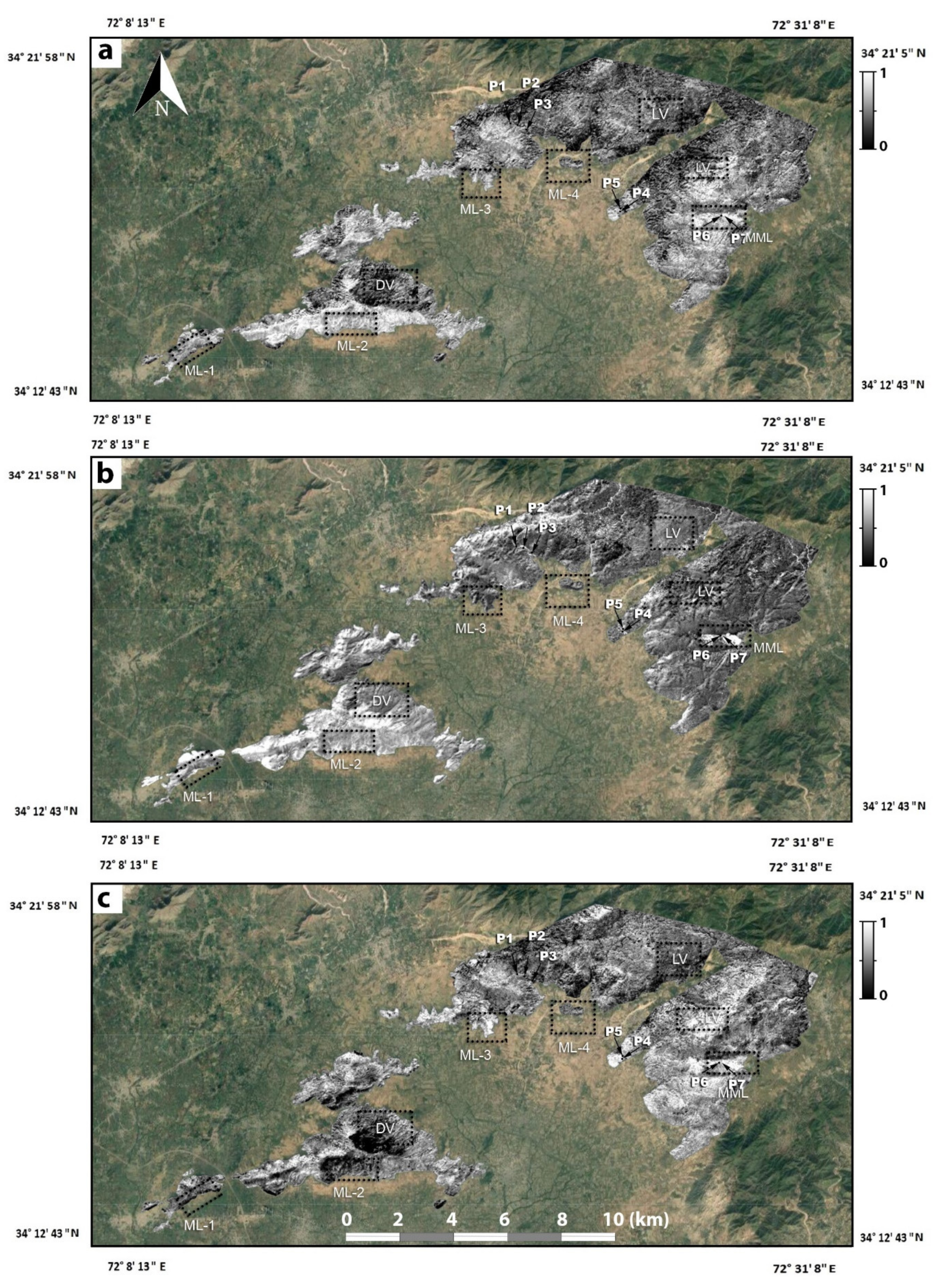
| S. No | Techniques | Field Points (Ground Truth) | Mining Leases (Ground Truth) | Accuracy | ||||||||||
|---|---|---|---|---|---|---|---|---|---|---|---|---|---|---|
| P1 (G) | P2 (G) | P3 (G) | P4 (G) | P5 (G) | P6 (M) | P7 (M) | ML1 (G) | ML2 (G) | ML3 (G) | ML4 (G) | MML (M) | |||
| 1 | Proposed weighted linear combination of FPCS components | G | G | G | G | G | M | M | G | G | G | G | M | 100% |
| 2 | FCC of PCs obtained after PCA applied to 17 raw bands from 3 data sources | VL | VL | S | G | G | G | G | G | G | G | VL | G | 44% |
| 3 | FCC of PCs obtained after PCA applied to 17 stretched bands from 3 data sources | VL | VL | G | G | G | M | M | G | G | G | G | M | 82% |
| Data Sources Selected Component | Description of Associated Bands of the Data Sources Associated Eigen Loadings of Selected Component | |||||
|---|---|---|---|---|---|---|
| Sentinel-2 | Blue B2 (0.49) | Green B3 (0.56) | Red B4 (0.665) | NIR B8 (0.842) | SWIR1 B11 (1.570–1.65) | SWIR2 B12 2.115–2.29) |
| PC5 of the stretched data | 0.1631 | −0.0168 | −0.1254 | −0.0206 | −0.2979 | −0.9317 |
| ASTER | VNIR B1 (0.52–0.6) | VNIR B2 (0.63–0.69) | NIR B3N (0.78–0.86) | TIR 1 B10 (8.12–8.47) | TIR 2 B11 (8.47–8.82) | TIR 3 B12 (8.92–9.27) |
| PC2 of the raw data | −0.2282 | −0.2717 | −0.2819 | −0.1059 | 0.4852 | 0.2368 |
| Landsat-8 | NIR B5 (0.85–0.88) | SWIR1 B6 (1.57–1.66) | SWIR2 B7 (2.11–2.29) | TIR1 B10 (10.6–11.19) | TIR2 B11 (11.5–12.51) | |
| PC5 of the stretched data | −0.4988 | −0.4413 | −0.0721 | 0.5150 | 0.5347 | |
| Data Sources Selected Component | Description of Associated Bands of the Data Sources Associated Eigen Loadings of Selected Component | |||||
|---|---|---|---|---|---|---|
| Sentinel-2 | Blue B2 (0.49) | Green B3 (0.56) | Red B4 (0.665) | NIR B8 (0.842) | SWIR1 B11 (1.570–1.65) | SWIR2 B12 (2.115–2.29) |
| PC2 of the raw data | −0.1879 | −0.1615 | −0.3477 | 0.8675 | 0.1512 | −0.2055 |
| PC5 of the stretched data | 0.2935 | 0.2873 | −0.2607 | 0.6071 | 0.5116 | 0.3644 |
| ASTER | VNIR B1 (0.52–0.6) | VNIR B2 (0.63–0.69) | NIR B3N (0.78–0.86) | TIR 1 B10 (8.12–8.47) | TIR 2 B11 (8.47–8.82) | TIR 3 B12 (8.92–9.27) |
| PC5 of the stretched data | −0.3434 | −0.1360 | −0.4276 | −0.3374 | −0.6024 | −0.4515 |
Publisher’s Note: MDPI stays neutral with regard to jurisdictional claims in published maps and institutional affiliations. |
© 2021 by the authors. Licensee MDPI, Basel, Switzerland. This article is an open access article distributed under the terms and conditions of the Creative Commons Attribution (CC BY) license (https://creativecommons.org/licenses/by/4.0/).
Share and Cite
Din, S.U.; Muhammad, K.; Khan, M.F.A.; Bashir, S.; Sajid, M.; Khan, A. A Fusion of Feature-Oriented Principal Components of Multispectral Data to Map Granite Exposures of Pakistan. Appl. Sci. 2021, 11, 11486. https://doi.org/10.3390/app112311486
Din SU, Muhammad K, Khan MFA, Bashir S, Sajid M, Khan A. A Fusion of Feature-Oriented Principal Components of Multispectral Data to Map Granite Exposures of Pakistan. Applied Sciences. 2021; 11(23):11486. https://doi.org/10.3390/app112311486
Chicago/Turabian StyleDin, Shahab Ud, Khan Muhammad, Muhammad Fawad Akbar Khan, Shahid Bashir, Muhammad Sajid, and Asif Khan. 2021. "A Fusion of Feature-Oriented Principal Components of Multispectral Data to Map Granite Exposures of Pakistan" Applied Sciences 11, no. 23: 11486. https://doi.org/10.3390/app112311486
APA StyleDin, S. U., Muhammad, K., Khan, M. F. A., Bashir, S., Sajid, M., & Khan, A. (2021). A Fusion of Feature-Oriented Principal Components of Multispectral Data to Map Granite Exposures of Pakistan. Applied Sciences, 11(23), 11486. https://doi.org/10.3390/app112311486