Article

‘SRS’ R Package and ‘q2-srs’ QIIME 2 Plugin: Normalization of Microbiome Data Using Scaling with Ranked Subsampling (SRS)

1
Centro de Oncologia Molecular, Hospital Sírio-Libanês, São Paulo 01308-060, Brazil
2
Departamento de Bioquímica, Instituto de Química, Universidade de São Paulo, São Paulo 05508-900, Brazil
3
Molecular Phytopathology and Mycotoxin Research, Faculty of Agricultural Sciences, University of Goettingen, 37077 Goettingen, Germany
4
Julius Kühn Institute (JKI)—Federal Research Centre for Cultivated Plants, Institute for Ecological Chemistry, Plant Analysis and Stored Product Protection, 14195 Berlin, Germany
*
Authors to whom correspondence should be addressed.
These authors contributed equally to this work.
Appl. Sci. 2021, 11(23), 11473; https://doi.org/10.3390/app112311473
Submission received: 1 November 2021 / Revised: 23 November 2021 / Accepted: 29 November 2021 / Published: 3 December 2021
(This article belongs to the Section Applied Microbiology)

Abstract

:
Several ecological data types, especially microbiome count data, are commonly sample-wise normalized before analysis to correct for sampling bias and other technical artifacts. Recently, we developed an algorithm for the normalization of ecological count data called ‘scaling with ranked subsampling (SRS)’, which surpasses the widely adopted ‘rarefying’ (random subsampling without replacement) in reproducibility and in safeguarding the original community structure. Here, we describe an implementation of the SRS algorithm in the ‘SRS’ R package and the ‘q2-srs’ QIIME 2 plugin. We also provide accessory functions for dataset exploration to guide the choice of parameters for SRS.

1. Introduction

High-throughput sequencing of taxonomically informative loci of microbial genomes by amplicon sequencing dramatically improved our understanding of microbial communities. Microbiome research expanded into all microbial habitats on earth, including the human intestine (e.g., [1]), soils (e.g., [2]), and deep-sea sediments (e.g., [3]). A range of bioinformatic tools and platforms as well as reference databases have been developed to enable the extraction of biological insight from the large amounts of data generated by multiplexed amplicon sequencing. The number of sequence counts per sample (sequencing depth) obtained from such sequencing runs can vary by orders of magnitude [4]. Those variations are technical artifacts caused by unequal pooling of samples prior to multiplexed sequencing runs and varying sequencing efficiencies. This contributes to biased estimates of several parameters assessed in microbiome analysis, such as alpha and beta diversity, and relative abundances of taxa.
Fortunately, variations in sequencing depth can be computationally compensated by normalization of sequence counts per sample, a step that has become essential in processing amplicon sequencing data. Traditionally, rarefying was used for this. In 2014, however, McMurdie and Holmes [4] demonstrated that rarefying is statistically inadmissible for the normalization of microbiome count data. Although the work of McMurdie and Holmes [4] received a lot of attention, rarefying is still frequently used in current microbiome studies, likely due to a lack of suitable alternatives. This motivated us to develop the scaling with ranked subsampling (SRS) algorithm, which outperforms rarefying for diversity analysis and relative abundance estimates, as recently shown [5].
Because unequal sampling depth is a problem inherent not only to microbiome research but to all studies based on ecological count data, we introduced SRS as a tool for the normalization of ecological count data and successfully applied it to microbiome analysis [5]. Yet, the implementation of SRS in bioinformatic platforms was missing.
In this work, we introduce an R package (‘SRS’) and a QIIME 2 plugin (‘q2-srs’) for the normalization of microbiome count data using SRS. Furthermore, we improve the original SRS algorithm and add features to visualize and evaluate the results. Finally, we provide an example for microbial ecologists that aim to normalize microbiome count data obtained by amplicon sequencing.

2. Theory

Ecological surveys and microbiome analysis by amplicon sequencing yield so-called species count data, which typically populate matrices with species represented by rows and samples represented by columns. Species are taxa (e.g., genera or binomial names), nucleotide sequences (ASVs), or sets of sequences grouped by similarity (OTUs). Samples are specimens of material (e.g., water or soil) or individuals or their parts (e.g., a plant or a bird intestine) distinguished by space-time attributes or treatments. The matrices are filled with nonnegative integers, which are designated counts. Analysis of count data is also used in other research fields such as bibliographic analysis, sociology of crime, and epidemiology of rare diseases. We suggest that study areas unrelated to ecology may also benefit from concepts developed for species count data in ecology.
The purpose of normalization is to convert a species count matrix into a normalized matrix, which has an equal dimension and is filled with integers such that the sum of counts of all species in each sample equals a pre-defined value, which we designate Cmin, and the structure of the normalized matrix approximates the structure of the original matrix. The criteria for the approximation may differ but a key principle is that relative frequencies of counts of the normalized matrix are as close as possible to the relative frequencies of counts in the original matrix. A relative frequency is obtained by dividing the count for a particular species in a particular sample by the sum of counts for all species in that sample. Different implementations of the criterion of matching relative frequencies are conceivable. The simplest option is to construct a normalization matrix minimizing the sum of absolute values of pairwise differences between the relative frequencies. This approach, however, ignores the effect of sampling error on the accuracy of relative frequencies. In the first approximation, the coefficient of variation of a count is proportional to the inverse of the square root of the count. Therefore, frequencies may be weighted by the inverse square root of counts. Depending on the purpose of the study, for instance, regarding the importance of rare species, other weighing may be more adequate.
Regardless of the criterion used to minimize the differences among sets of relative frequencies of species, which are colloquially referred to as “population structure”, the task is an optimization problem under integer constraint, which is a special kind of integer programming problem. Let assume sampling data for J species in K samples with counts collected in a J × K matrix. Let C ( j , k ) denote the count of species j in sample k and F ( j , k ) the relative frequency of species j in sample k:
F ( j , k ) = C ( j , k ) i = 1 J C ( i , k ) .
Let C ( j , k ) n o r m denote the normalized count of species j in sample k. The constraint of equal total species count per sample implies
i = 1 J C ( i , 1 ) n o r m = i = 1 J C ( i , 2 ) n o r m = = i = 1 J C ( i , K ) n o r m = C min .
Conversion of C ( j , k ) into C ( j , k ) n o r m satisfying this constraint and leading to frequencies derived from the normalized matrix
F ( j , k ) n o r m = C ( j , k ) n o r m i = 1 J C ( i , k ) n o r m
as close as possible to the original frequencies F ( j , k ) is the purpose of normalization. The normalized matrix minimizes the sum of differences between original frequencies and frequencies derived from the normalized counts, while frequencies may be weighted by factor r and the differences may be raised to power s:
i = 1 J r | F ( i , k ) F ( i , k ) n o r m | s .
As a weighting factor, 1 can be used for equal weights or C ( i , k ) to compensate for differences in the sampling error. As a power s, 1 can be used for absolute differences or 2 in line with the least-square concept. Weighing or raising the difference to a power, however, rarely affects the results, as shown by the following example. Let C ( k ) be a column vector of species counts for sample k and C ( k ) T its transposition into a row vector:
C ( k ) T = ( 2 ,   4 ,   30 ,   600 ,   0 ,   27 ,   231 ) .
The total species count in sample k is 894. After normalization to Cmin = 100, the same normalized counts are obtained for all combinations of optimization parameters:
r { 1 , C ( i , k ) } , s { 1 , 2 } :      C ( k ) T = ( 0 ,   1 ,   3 ,   67 ,   0 ,   3 ,   26 ) .
The normalization was conducted by comparing 7-tuples of nonnegative integers such that each term varied from zero to
C ( j , k ) 100 894 + 5
while the sum of terms was Cmin. Exhaustive enumeration of this kind is not feasible for real-world data. In 2014, Cont and Heidari suggested an algorithm solving this optimization problem with the complexity O(n log n), n being the number of species, but their preprint has not been subjected to a peer review yet [6]. The SRS algorithm [5], which has the complexity of O(n), generated the same results in this example.
SRS is an empirical algorithm that does not rely on comparison of relative frequencies of raw and normalized counts. On real as well as simulated count data, SRS was, however, shown to perform substantially better than normalization by rarefying [5].

3. Method

3.1. Principle of SRS

The SRS algorithm performs scaling followed by ranked subsampling.
  • Scaling: feature counts (such as OTUs (operational taxonomic units), ASVs (amplicon sequence variants), or clades) are scaled sample-wise so that the sum of the scaled counts (Cscaled) for each sample is equal to the desired number of counts (Cmin).
  • Ranked subsampling: the scaling step produces fractional values that must be converted into counts (integers). To do this, the Cscaled for each feature is split into the floor (Cint) and fractional part (Cfrac) of Cscaled. Because Cmin = ΣCscaled = ΣCint + ΣCfrac, it follows that Cmin ≥ ΣCint. Therefore, ΔC Cfrac values (where ΔC = Cmin − ΣCint) must be converted into additional counts (integers) so that Cmin can be reached. To do so, Cfrac values are ranked. Next, from the highest to the lowest rank, a count for each feature is added until ΔC counts have been added. After this step, all samples will have been normalized to Cmin counts.
  • Special cases: (i) when Cfrac values involved in picking ΔC counts share the same rank across features, the counts are added for features based on the respective Cint ranks; (ii) when both Cfrac and its respective Cint values involved in picking ΔC counts share the same ranks across features, the counts are assigned randomly (without replacement). The specification of the seed that initializes the random process enables reproducible results.

3.2. ‘SRS’ R Package

3.2.1. SRS-Function

The SRS algorithm was implemented as the SRS-function in the ‘SRS’ R package (https://CRAN.R-project.org/package=SRS (accessed on 1 November 2021)). As an extension of the original SRS algorithm published by Beule and Karlovsky [5], SRS as implemented in version 0.2.2 of the package enables reproducible results in case SRS uses random subsampling without replacement by specifying the seed that initializes the random process (set.seed). The default settings of the SRS-function (as of version 0.2.2) are:
SRS(data, Cmin, set_seed = TRUE, seed = 1)
where data is the input data (e.g., an OTU table), with samples distributed column-wise, Cmin is the number of counts to which all samples will be normalized (Cmin), set_seed enables the use of the set.seed-function, and seed specifies the seed used by set.seed to initialize the random process.

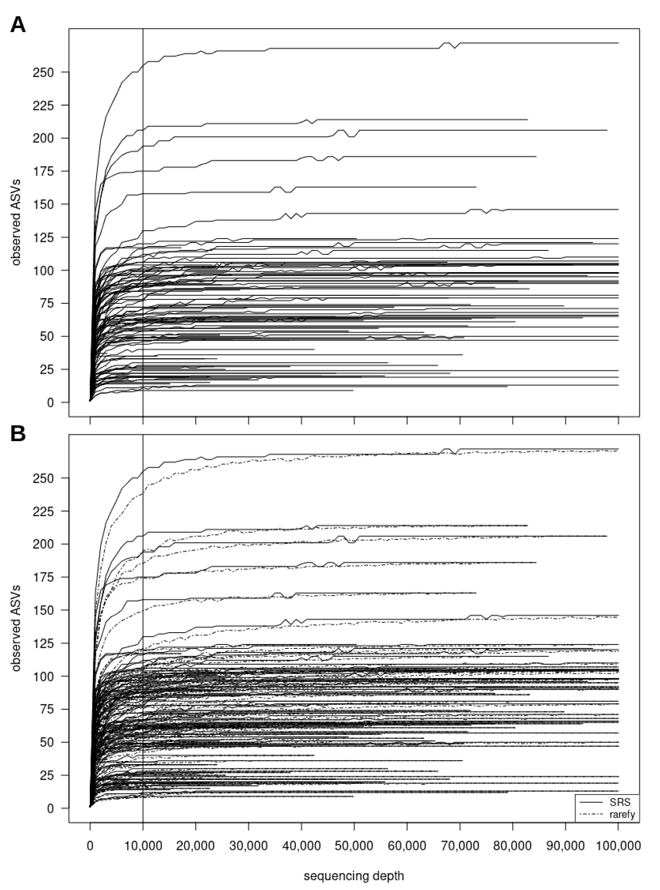
3.2.2. SRScurve-Function

In analogy to rarefaction curves, the SRScurve-function of the ‘SRS’ R package plots the number of observed unique features (observed richness) against the number of sampled counts utilizing the SRS-function (SRS curves). In addition to observed richness, different alpha diversity metrics (Shannon, Simpson, and inverse Simpson indices as implemented in the diversity-function of the ‘vegan’ R package [7]) can be selected to generate SRS curves. Furthermore, SRScurve allows a direct comparison to averaged repeated rarefying. The default settings of the SRScurve-function (as of version 0.2.2) are:
SRScurve(data, metric = “richness”, step = 50, sample = 0,
   max.sample.size = 0, rarefy.comparison = FALSE,
     rarefy.repeats = 10, rarefy.comparison.legend = FALSE,
     xlab = “sample size”, ylab = “richness”, label = FALSE,
col, lty,…)
where data is the input data (e.g., an OTU table), metric selects the alpha diversity metric to be plotted (“richness” = observed richness; “shannon” = Shannon index; “simpson” = Simpson index; “invsimpson” = inverse Simpson index), step specifies the step size at which the alpha diversity metric are sampled, sample specifies the cutoff-level to visualize trade-offs between cutoff-level and alpha diversity, max.sample.size specifies the maximum sample size to which SRS curves are drawn (the default does not limit the maximum sample size), rarefy.comparison enables comparison of SRS curves to rarefying, rarefy.repeats specifies the number of repeats used for rarefying, rarefy.comparison.legend, xlab, ylab, label, col, lty, and… are graphical parameters.

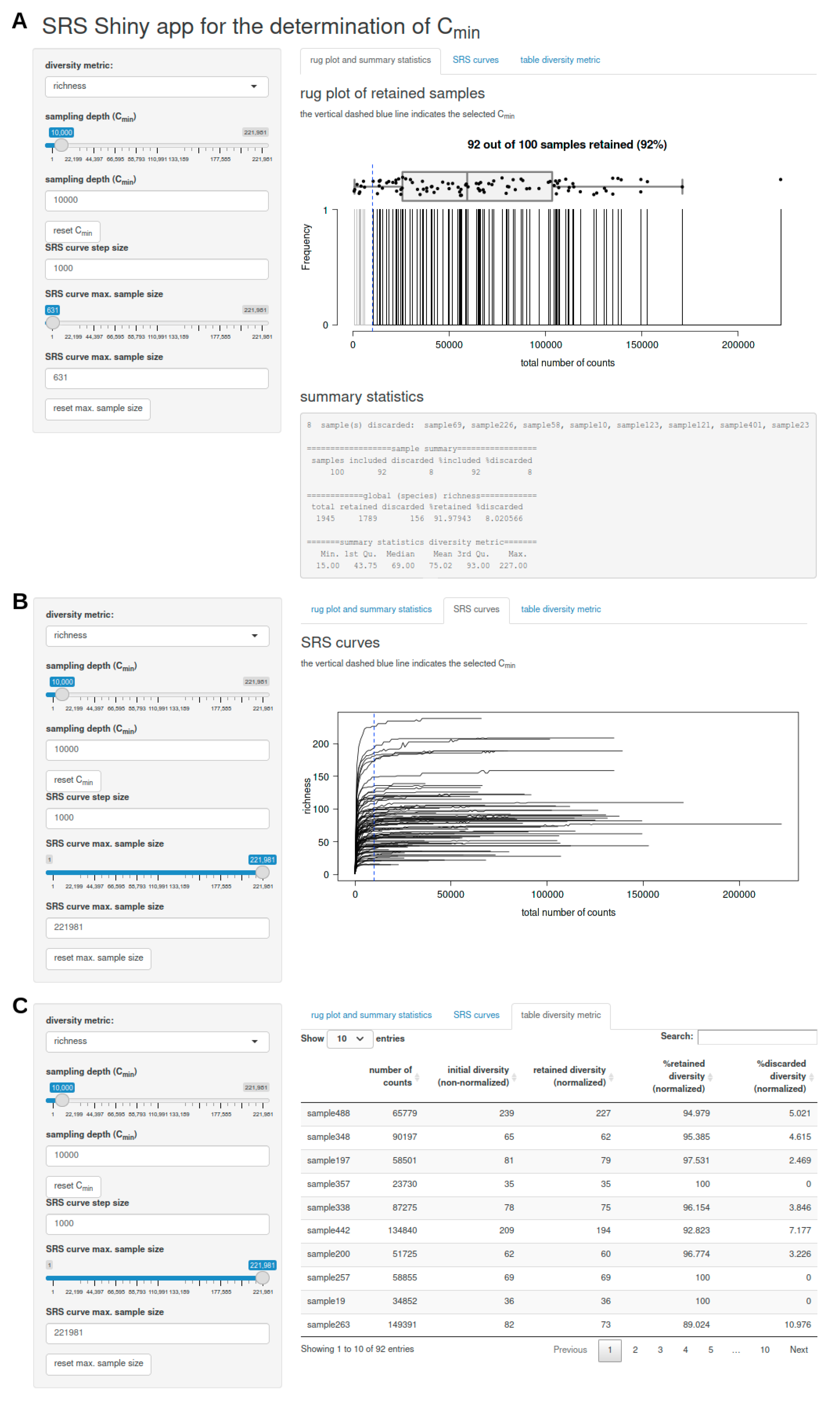
3.2.3. SRS.shiny.app-Function

The SRS.shiny.app-function of the ‘SRS’ R package launches a Shiny app for SRS in the default web browser to determine Cmin. The app utilizes the SRScurve-function and enables the selection of four diversity metrics (see metric in SRScurve) that will be returned at different Cmin. The selection of Cmin is interactive through a slider or an interconnected numeric text field. In response to the selected Cmin, the app returns
  • a rug plot that shows the distribution of the number of counts per sample and displays discarded samples as well as summary statistics (including a list of discarded samples and descriptive statistics of the global feature richness and selected alpha diversity metric of the input dataset) in response to the selected Cmin (Figure 1A),
  • a plot of SRS curves (SRScurve-function) that respond to the selected step size (step) and maximum sample size (max.sample.size) (Figure 1B), and
  • an interactive table with sample names and the number of counts per sample as well as the initial diversity (non-normalized), retained diversity (normalized), %retained diversity (normalized), and %discarded diversity (normalized) of the selected alpha diversity metric in response to the selected Cmin (Figure 1C).
The default Cmin of the app is the lowest total number of counts per sample in the input data (no samples are discarded by default), which can be restored within the app using the reset Cmin-button. The default maximum sample size equals the default setting of Cmin and can be restored using the reset max. sample size-button. The default step size for SRS curves is 1000. The default setting of the SRS.shiny.app-function (as of version 0.2.2) is:
SRS.shiny.app(data)
where data is the input data (e.g., an OTU table).

3.3. ‘q2-srs’ QIIME 2 Plugin

The ‘q2-srs’ QIIME 2 plugin (https://library.qiime2.org/plugins/q2-srs (accessed on 1 November 2021)) allows straightforward SRS algorithm incorporation into QIIME 2 pipelines. Because its implementation wraps up the ‘SRS’ R package, its functionalities are analogous to those presented in the previous section.
Specifically, ‘q2-srs’ features the QIIME 2 actions SRS and SRScurve, which mirror the ‘SRS’ R package SRS-function and SRScurve-function, respectively, with the same behaviour and default parameters as presented in the previous section. The command-line interface commands for the use of the SRS- and SRScurve-functions within QIIME 2 environment are, respectively, qiime srs SRS and qiime srs SRScurve. Finally, despite the ‘q2-srs’ QIIME 2 plugin not having a SRS.shiny.app-function counterpart, an online version of the SRS Shiny app (https://vitorheidrich.shinyapps.io/srsshinyapp/ (accessed on 1 November 2021)) is provided for ‘q2-srs’ users.

4. Results and Discussion

In both the R package as well as the QIIME 2 plugin, we modified the original SRS algorithm by specifying a seed that initializes the random process (set.seed) in cases where the SRS uses random subsampling without replacement of the lowest Cfrac. The random step in SRS is rare and negligible for complex microbiome data, as noted previously [5]. This rather minor modification, however, ensures the reproducibility of SRS, which is essential for microbiome analysis [8].
As an example of microbiome count data normalization using SRS, we utilized a bacterial 16S rRNA gene amplicon sequencing dataset comprising 494 samples derived from an ongoing oral microbiome study. The dataset was processed in QIIME 2 [9]. After anonymization of samples and ASVs, an ASV table comprising a random subset of 100 samples was analyzed. The visualization of SRS curves revealed that the observed ASVs did not decay steadily with decreasing number of reads (Figure 2A). This is due to the way the ranked fractional values (Cfrac) are chosen: depending on the scaling factor, an ASV with an integer value (Cint) of zero may or may not be chosen by ranked subsampling due to its Cfrac, causing a reproducible zigzag behaviour in the observed number of species. The magnitude of the zigzag observed in SRS curves depends on the data structure (balance between rare and abundant ASVs). Despite the zigzag behaviour, the observed ASV richness was frequently observed to be higher after SRS as compared to rarefying (Figure 2B). Therefore, we recommend the use of the SRS Shiny app (SRS.shiny.app-function) prior to SRS for the determination of Cmin for users working in the R environment. QIIME 2 users are also encouraged to utilize .qza files in the SRS Shiny app (https://vitorheidrich.shinyapps.io/srsshinyapp/ (accessed on 1 November 2021)).
Since its implementation in accessible platforms, SRS has been used to normalize several microbiome datasets obtained from different environments such as animal guts [10], soils [11], oceans [12], and laboratory cultures [13]. McMurdie and Holmes [4] clearly demonstrated that rarefying should not be used to normalize microbiome count data; thus, we suggest that future studies should compare SRS to commonly used normalization techniques other than rarefying.

Author Contributions

Conceptualization, V.H., P.K. and L.B.; methodology, V.H., P.K. and L.B.; software, V.H. and L.B.; validation, V.H., P.K. and L.B.; formal analysis, V.H. and L.B.; investigation, V.H., P.K. and L.B.; resources, V.H., P.K. and L.B.; data curation, V.H. and L.B.; writing—original draft preparation, V.H. and L.B.; writing—review and editing, P.K.; visualization, V.H. and L.B.; supervision, P.K.; project administration, V.H., P.K. and L.B.; funding acquisition, V.H., P.K. and L.B. All authors have read and agreed to the published version of the manuscript.

Funding

This work was supported by the German Federal Ministry of Education and Research (BMBF) in the framework of the Bonares-SIGNAL project (funding codes: 031A562A and 031B0510A). V.H. was supported by Fundação de Amparo à Pesquisa do Estado de São Paulo (FAPESP, process No. 13996-0/2018).

Institutional Review Board Statement

The dataset analyzed here is provenient of a study that was conducted according to the guidelines of the Declaration of Helsinki, and approved by the Ethics Committee of Hospital Sírio-Libanês (protocol code: HSL 2016-08; date of approval: 18 February 2016).

Informed Consent Statement

Informed consent was obtained from all subjects involved in the study.

Data Availability Statement

The ASV table as well as the R script underlying the results of this study are available on GitHub (https://github.com/vitorheidrich/SRS_q2-srs_info (accessed on 1 November 2021)).

Acknowledgments

The authors thank Devon O’rourke for his suggestions.

Conflicts of Interest

The authors declare no conflict of interest.

References

  1. Yatsunenko, T.; Rey, F.E.; Manary, M.J.; Trehan, I.; Dominguez-Bello, M.G.; Contreras, M.; Magris, M.; Hidalgo, G.; Baldassano, R.N.; Anokhin, A.P.; et al. Human Gut Microbiome Viewed across Age and Geography. Nature 2012, 486, 222–227. [Google Scholar] [CrossRef] [PubMed]
  2. Fierer, N. Embracing the Unknown: Disentangling the Complexities of the Soil Microbiome. Nat. Rev. Microbiol. 2017, 15, 579–590. [Google Scholar] [CrossRef]
  3. Orsi, W.D. Ecology and Evolution of Seafloor and Subseafloor Microbial Communities. Nat. Rev. Microbiol. 2018, 16, 671–683. [Google Scholar] [CrossRef]
  4. McMurdie, P.J.; Holmes, S. Waste Not, Want Not: Why Rarefying Microbiome Data Is Inadmissible. PLoS Comput. Biol. 2014, 10, e1003531. [Google Scholar] [CrossRef] [Green Version]
  5. Beule, L.; Karlovsky, P. Improved Normalization of Species Count Data in Ecology by Scaling with Ranked Subsampling (SRS): Application to Microbial Communities. PeerJ 2020, 8, e9593. [Google Scholar] [CrossRef] [PubMed]
  6. Cont, R.; Heidari, M. Optimal Rounding under Integer Constraints. arXiv 2014, arXiv:1501.00014. [Google Scholar]
  7. Oksanen, J.; Blanchet, F.G.; Friendly, M.; Kindt, R.; Legendre, P.; McGlinn, D.; Minchin, P.R.; O’Hara, R.B.; Simpson, G.L.; Solymos, P.; et al. Vegan: Community Ecology Package. R Package Version 2.5-7. 2020. Available online: https://CRAN.R-project.org/package=vegan (accessed on 1 November 2021).
  8. Schloss, P.D. Identifying and Overcoming Threats to Reproducibility, Replicability, Robustness, and Generalizability in Microbiome Research. mBio 2018, 9, e00525-18. [Google Scholar] [CrossRef] [PubMed] [Green Version]
  9. Bolyen, E.; Rideout, J.R.; Dillon, M.R.; Bokulich, N.A.; Abnet, C.C.; Al-Ghalith, G.A.; Alexander, H.; Alm, E.J.; Arumugam, M.; Asnicar, F.; et al. Reproducible, Interactive, Scalable and Extensible Microbiome Data Science Using QIIME 2. Nat. Biotechnol. 2019, 37, 852–857. [Google Scholar] [CrossRef]
  10. Yang, J.; Park, J.; Jung, Y.; Chun, J. AMDB: A Database of Animal Gut Microbial Communities with Manually Curated Metadata. Nucleic Acids Res. 2021, gkab1009. [Google Scholar] [CrossRef] [PubMed]
  11. Beule, L.; Arndt, M.; Karlovsky, P. Relative Abundances of Species or Sequence Variants Can Be Misleading: Soil Fungal Communities as an Example. Microorganisms 2021, 9, 589. [Google Scholar] [CrossRef]
  12. Pontiller, B.; Pérez-Martínez, C.; Bunse, C.; Osbeck, C.M.G.; González, J.M.; Lundin, D.; Pinhassi, J. Taxon-Specific Shifts in Bacterial and Archaeal Transcription of Dissolved Organic Matter Cycling Genes in a Stratified Fjord. bioRxiv 2021. [Google Scholar] [CrossRef]
  13. Barreto Filho, M.M.; Walker, M.; Ashworth, M.P.; Morris, J.J. Structure and Long-Term Stability of the Microbiome in Diverse Diatom Cultures. Microbiol. Spectr. 2021, 9, e00269-21. [Google Scholar] [CrossRef] [PubMed]
Figure 1. User interface of the Shiny app for SRS (SRS.shiny.app-function of the ‘SRS’ R package version 0.2.2). (A) Rug plot showing the distribution of the number of counts per sample, discarded samples, and summary statistics; (B) plot showing SRS curves; (C) interactive table with sample names, the number of counts per sample, and summary statistics for the diversity metric.
Applsci 11 11473 g001
Figure 2. (A) SRS curves and (B) comparison of SRS curves and repeated rarefying (10 repeats) using the “richness” metric (SRScurve-function of the ‘SRS’ R package version 0.2.2). The vertical black solid line indicates the chosen number of counts (10,000) to which all samples will be normalized (Cmin).
Applsci 11 11473 g002
Publisher’s Note: MDPI stays neutral with regard to jurisdictional claims in published maps and institutional affiliations.

