Abstract
The modernization and optimization of current power systems are the objectives of research and development in the energy sector, which is motivated by the ever-increasing electricity demands. The goal of such research and development is to render power electronic equipment more controllable, to ensure maximal use of current circuits, system flexibility and efficiency, as well as the relatively easy integration of renewable energy resources at all voltage levels. The current revolution in communication technologies and the Internet of Things (IoT) offers us an opportunity to supervise and regulate the power grid, in order to achieve more reliable, efficient, and cost-effective services. One of the most critical aspects of efficient power system operation is the ability to predict energy load requirements, i.e., load forecasting. Load forecasting is essential for balancing demand and supply and for determining electricity prices. Typically, load forecasting has been supported through the use of Artificial Neural Networks (ANNs), which, once trained on a set of data, can predict future loads. The accuracy of the ANNs’ prediction depends on the quality and availability of the training data. In this paper, we propose novel data pre-processing strategies, which we apply to the data used to train an ANN, and subsequently evaluate the quality of the predictions it produces, to demonstrate the benefits gained. The proposed strategies and the obtained results are illustrated using consumption data from the Greek interconnected power system.
1. Introduction
A power system must be designed, constructed and controlled in such a way that it is safe, reliable, environmentally friendly, and practical; that is, it can supply high-quality electricity at the lowest possible price. The reliability of a power system is determined by the extent to which it covers the overall energy demands of consumers, even under temporal and local fluctuations in the load, i.e., the system should be able to respond to changes in the demand for active and reactive power on a continuous basis. The quality of electricity is assessed with reference to known limits for voltage and frequency variations, which are typically 5% and 0.5%, respectively.
For the power system to meet its operational criteria, it must be constantly managed and optimized through the implementation of various methods. System optimization adds a significant economic benefit, with major utilities saving hundreds of millions of dollars each year in fuel costs, increased operating efficiency and system security. Different optimization problems, such as economic transmission, unit engagement, hydrothermal scheduling, optimum power flow, maintenance scheduling, etc., have been realized in power system operation [1], using conventional and Artificial Intelligence (AI) techniques. The latter have proved especially valuable in rendering the power system ‘smarter’.
A central theme in smart energy systems is load forecasting, as it plays a critical role in many aspects of power system management and operation. Specifically, to schedule the effective operation and sustainable capital extension of an electric power distribution system, the system operator must be able to predict the need for power supply at various locations and at all times. During operation, power generation must increase or decrease in tandem with system load, and this on-demand power generation necessitates an adequate generation capacity. Knowing the load parameters in advance allows the electric utility operator to optimallmanage grid capacity [2]. Many critical operational decisions, such as power generation scheduling, fuel purchase scheduling, maintenance scheduling, and electricity transaction preparation, are dependent on electric load forecasting; hence, the accuracy of forecasts directly or indirecly impacts the overall economic viability and dependability of any electricity utility. In a deregulated environment, all concerned parties conduct load forecasting on a regular basis; hence, generation providers, transmission companies, Independent System Operators (ISOs), and Regional Transmission Organizations (RTOs) depend on accurate load forecasts to prepare, negotiate, and operate [3]. Approaches to the load forecasting problem distinguish between short-term (STLF), medium-term (MTLF), and long-term load forecasting (LTLF). Long-term predictions are generally necessary for the scheduling of power systems, medium-term predictions are required for maintenance and planning of fuel supply, and short-term predictions are required for the daily operation of the power system.
Short-term load forecasting was traditionally performed using approaches such as time series models, regression, and Kalman filtering. A variety of Artificial Intelligence algorithms, Deep Learning and Neuro-Fuzzy methods have been developed and applied in the field of electricity systems for optimal operation and management of the power system, load forecasting and electricity price forecasting. For instance, Alamaniotis et al. propose a Gaussian Process Regression (GPR) and a Relevance Vector Regression (RVR) to approach the load forecasting issue based on historical load data for New England’s power system [4]. Kontogiannis et al. [5] propose the design of a fuzzy control system that uses environmental data, such as weather parameters, to achieve minimal energy consumption in buildings. This fuzzy control system relies on decision tree metrics to determine the importance of data features. In a similar effort, to promote AI methods based on RVRs, Alamaniotis et al. reuse the historical data of New England’s power system to forecast the price of electricity the next day [6]. In a later attempt [7], the author proposes a novel hybrid methodology to address the same issue. Initially, it uses RVRs to determine the price of the next day’s electricity. It then uses these prediction results in conjunction with a micro-genetic algorithm to enhance the prediction and determine the final value.
The first attempts to address the issue of hourly load prediction using Multi-Layer Perceptrons (MLPs) appeared in the early 1990s. In [8] Park et al. provide a theoretical analysis and mathematical background for the application of three-layer perceptrons to load prediction. Using historical load and temperature data, their proposed system managed to produce three different forecast variables (peak load, total daily load and hourly load) with Mean Average Percentage Error (MAPE) values of less than 3%. In an effort to extend the existing techniques, Kun-Long Ho et al. applied an adaptive learning algorithm to yield more accurate MLP predictions [9]. A different approach is presented in [10], where a minimum distance measurement is used to find the correlations of the data used as neuronal inputs. The differences lie in the fact that input data include information about the total load and maximum and minimum temperature of the previous days, as well as the predicted maximum and minimum temperature for the forecast day, which, together with an enhanced learning algorithm, produce better prediction results. In a more sophisticated approach, Kandil et al. used a simple MLP for short-term load forecasting [11]. In this paper, they focused on increasing the amount of important and highly correlated data used as neural network inputs. Thus, the authors used an hour indicator, day indicator, and the estimated temperature at hour k, k-1 and k-2 as variable inputs. Special emphasis is given to the fact that historical loads are not used as inputs.
A first attempt at short-term load forecasting based on the data of the Greek power system is presented in [12]. A fully connected three-layer feedforward ANN consisting of 63 input neurons, 24 hidden neurons and 24 output neurons was proposed by Bakirtzis et al. to predict the hourly values of the next day’s loads. Mandal et al., based on a similar range of days to the predicted day, use a solid method to predict energy prices several hours ahead, and for load forecasting [13]. They measured the correlation coefficient between the data and then integrated them into a three-layer MLP, which was trained with the backpropagation algorithm, using historical half-hourly data for the Victoria electricity sector. This study, without accounting for variables such as weather conditions and special status days, offered a more accurate approach to the STLF issue compared to previous, simpler methods. Another work related to STLF for the Greek Intercontinental Power System is presented in [14]. In their work, Tsekouras et al. compared various neural network training algorithms to predict hourly load demand by measuring the MAPE of each separately. The proposed neural network creation does not significantly differ in terms of structure, but it uses pre-processed input data. Such pre-processing is achieved via a normalization function proposed by the authors. Alamaniotis and Tsoukalas [15] presented a data-driven method for minutely active power forecasting based on Gaussian processes, highlighting the importance of minute predictions, while Kontogiannis et al. [16] presented a baseline performance comparison of neural network models for minutely active power forecasts derived from residential data.
Another category of neural networks that has interested the research community in recent decades and is directly applicable to load prediction are Radial Basis Function Networks (RBFNs). An initial analysis of the application of RBFNs to short-term load forecasting is presented in [17]. The proposed model is applied to STLF using load data of an Australian region from January to August 2004, yielding satisfactory results. In [18], Gontar et al. emphasizing the special importance and usefulness of RBFNs, recorded the results obtained by inputting load data for Crete. To reflect the seasonality of the data, they proposed the creation of four neural networks, one for each season. A fifth neural network was used to predict the loads on special days and the weekend. A comparative study using RBFNs is described in [19]. The authors, trying to achieve better a generalization of data, faster execution time and lower prediction error, considered the application of various algorithms for the training of neural networks. To evaluate the different learning techniques, they compared the prediction results obtained from RBFNs to those of Decay Radial Basis Function Networks (DRBFN), Support Vector Regression (SVR), Extreme Learning Machine (ELM), Improved Second-Order algorithm (ISO) and Error Correction algorithm (ErrCor).
Another approach to STLF with the application of hybrid models is presented in [20]. The researchers suggest the use of wavelet fuzzy neural networks (WFNN) and modified fuzzy neural networks (FNCI) to predict the next hour’s load, and they used load data from the Northern Region Load Dispatch Center in Delhi, India, as well as temperature, wind speed and humidity data, to evaluate their proposed hybrid models, yielding better prediction results than the traditional ANFIS model, which has been extensively used in the literature. In [21], Panapakidis proposes a robust hybrid model to forecast day-ahead and hour-ahead load predictions by using hourly load values of 10 buses of the Greek Power System located in the area of Thessaloniki, North Greece. The hybrid model is based on the combination of historical load and temperature data clustering and embedding in an MLP neural network. Specifically, the author recommends using the minCEntropy clustering algorithm on the training set to formulate k clusters. A different ANN is used for each subset. As a result, the data from the corresponding clusters are used to train k ANNs. The Euclidean distance is used to relate each pattern in the test set to k centroids, and the results are fed into the corresponding ANN.
In the spirit of previous researchers, an innovative approach to load prediction was described in [22]. Dong et al. proposed the implementation of a convolutional neural network (CNN) enhanced with K-means clustering to achieve higher scalability in the data and reduce the error rate in the forecast. Another hybrid load prediction system is described in detail in [23], where the authors emphasize the importance of pre-processing load data and propose an improved neural network learning algorithm. The data entered in the modification model refer to historical load data per hour and exogenous data that directly affect the load behaviour, such as temperature and humidity. The Min-Max normalization is applied, so that their values range between 0 and 1. Then, the data that show a greater correlation are entered into an MLP neural network, which is trained with a Modified Harmony Search (MHS) algorithm. In the category of hybrid models, Ekonomou et al. proposed a load forecasting model based on the combination of MLP neural networks and wavelet analysis [24]. The researchers manipulated historical load data from the Bulgarian power system grid as time series and applied a wavelet de-noising algorithm to remove their noise and split them into signals with different frequencies. In [25], K-shape is proposed as a new clustering technique to categorize consumers based on their load consumption behaviour. Another hybrid approach is described in [26]. The researchers use various machine learning algorithms to optimize the data they use in short-term load forecasting. Initially, they use the load data as time series and decompose them based on the Intrinsic Mode Function (IMF) technique. Then, with the help of the Particle Swarm Optimization (PSO) algorithm, data are filtered and used by the Extended Kalman Filter (EKF), Extreme Learning Machine with Kernel (KELM) for STLF. The authors conclude that this approach yields an acceptable forecasting accuracy and time performance. Likewise, [27] uses day- or week-ahead load data to create clusters, which are fed to an ANN. The errors that result from comparing this data with the actual ones are fed to a WNN, where the final prediction and the various error metrics are calculated. This process is repeated for various machine learning approaches. The results of these techniques are compared with the MAPE and the normalized Root Mean Square Error (nRMSE), where the approach with the least error is preferable.
Remaining in the hybrid model category, Massaoudi et al. propose a new technique for daily load forecasting based on a model that integrates Extreme Gradient Boosting (XGB), Light Extreme Gradient Boosting (LGBM), and MLP [28]. This combination produces MAPE values close to 2.69%. A K-Medoids clustering approach is used in conjunction with several deep learning prediction models in [29]. To reach 7.18% MAPE for the prediction of the following day’s load, the authors employ Autoregressive Integrated Moving Average (ARIMA), Deep Neural Networks (DNN), and Long Short-Term Memory (LSTM), as well as an advanced data scaling strategy. In addition to the above work, Lizhen et al. propose a hybrid neural network model that combines the Gated Recurrent Unit (GRU) and convolutional neural networks (CNN) for feature extraction of time series data [30]. The authors do not place a high level of importance on pre-processing the input data utilized by the GRU-CNN forecasting model, and the MAPE result is 2.88%. Similarly, Farsi et al. studied STLF using a Parallel LSTM-CNN network (PLCNet) [31]. The input data were scaled using the traditional min-max approach, yielding a MAPE of 2.08% for the prediction.
The above papers are some of the extensive literature on the application of various kinds of neural networks to short-term load forecasting. The bibliography is constantly increasing as new deep learning methods are tried. The effects produced by the various forms of data normalization, the various activation functions, and the various morphologies of neural networks are presented in [32,33,34].
This paper presents two innovative data pre-processing techniques applied to short-term load forecasting using artificial neural networks, beyond the simple and min–max scaling procedures. The two primary pre-processing strategies that were suggested concentrate on the gravity of particular neural network input variables in relation to output variables, resulting in superior prediction outcomes compared to traditional methods. Compared to existing studies using data from the Greek interconnected system, this method produces improved results in terms of Mean Squared Error (MSE), Mean Absolute Error (MAE) and MAPE.
2. Materials and Methods
2.1. Proposed Approach for STLF
Following a thorough review of the literature, two innovative data processing techniques are suggested, which differ from earlier work in that they place emphasis on specific input data, and their impact on the output variables of the neural network. The predictions obtained from such pre-processed input lead to increased accuracy, as is demonstrated by the results obtained. The next day’s load forecast, using historical data from previous days and the previous hour, as well as the structure of the neural networks used, are discussed in detail in this section.
2.2. Implementation for Short Term Load Forecasting
The data used in this study came from the Greek power system during the period 2013–2017 and refer to hourly load values. To make a more accurate forecast, weather data, such as temperature, were used in addition to the historical data of the loads. Data is separated into training and test sets in a ratio of 80% to 20%. Hence, the training set comprises data for the years 2013–2016, and the predictions produced are compared to data for year 2017 (test set). The neural networks employed were built using the Python programming language and specifically the library scikit-learn.
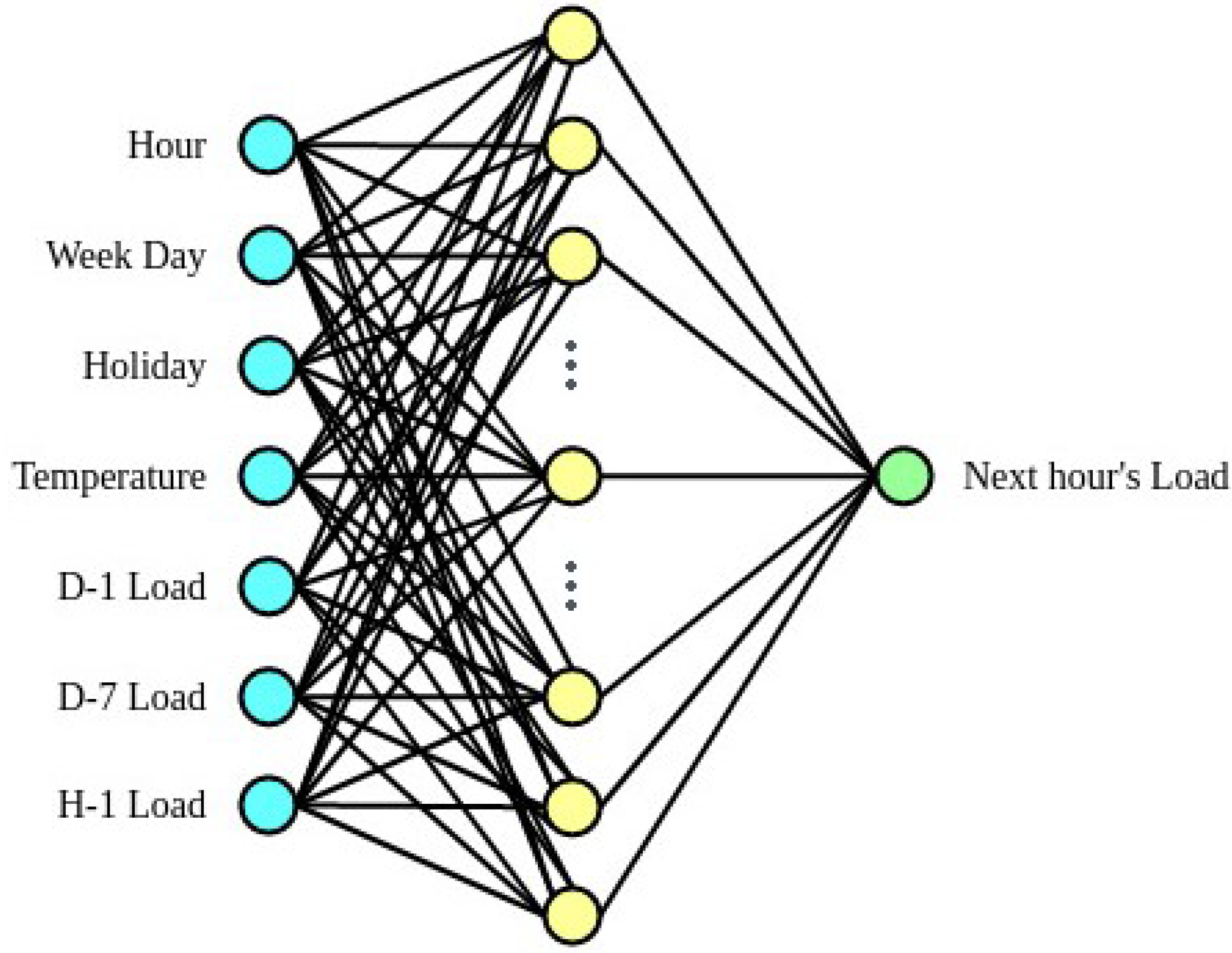
A modified MLP neural network is used to predict the hourly value of the load. A new input variable called is employed that refers to the value of the load in the hour preceding that for which the prediction is made. Since the behaviour of the hourly value of the load is represented with greater precision knowing the load of the Greek interconnected system in the previous hour, the inclusion of this component improves the model prediction. The improved neural network model consists of the following input variables:
- Hour: The time of day for which the load forecast will be made. The time is expressed as an integer with values ranging from 0 to 23.
- Week Day: It’s a characteristic coding to decide the day of the week. The coding is done with integers ranging from 1 to 7, with 1 denoting Sunday, 2 denoting Monday, and so on.
- Holiday: Binary coding is used to indicate whether a day is a holiday or a working day. The number 1 is used to designate Greek state holidays, such as national anniversaries and major religious holidays, as well as weekends. The other days, on the other hand, are coded with number 0.
- Temperature: The hourly value (in Celsius) of the temperature of the day for which the load is forecast.
- D-1 Load: The load value of the day preceding the one for which prediction is made, at the corresponding time. For example, if the MLP neural network predicts Wednesday at 17:00 then the value of Tuesday load at 17:00 is entered as input to the neural network.
- D-7 Load: The value of the load at the corresponding time on the same day of the previous week. If the load prediction for Wednesday 12 May 2017 at 17:00 is the output of the neural network, then the value of the load for Wednesday 5 May 2017 at 17:00 is entered as the neural network’s input.
- H-1 Load: The value of the previous hour’s load on which the forecast is based. If the load prediction for Wednesday 12 May 2017 at 17:00 is the neural network’s output, then the value of the load on Wednesday 12 May 2017 at 16:00 is entered as the neural network’s input.
The architecture of the MLP neural network that was used to predict the hourly value of the load is shown in Figure 1. An input layer, a hidden layer, and an output layer represent the three layers of a neural network. Seven neurons make up the input level. Each neuron is associated with one of the variables listed above. There are 100 neurons in the hidden layer. The value 100 was chosen experimentally as it was found to produce better predictive values by dramatically reducing error. As can be seen from the literature, neural networks with a single hidden layer address the STLF problem quite accurately. The output layer is composed of a single neuron and refers to the hourly load value for which the prediction is developed.
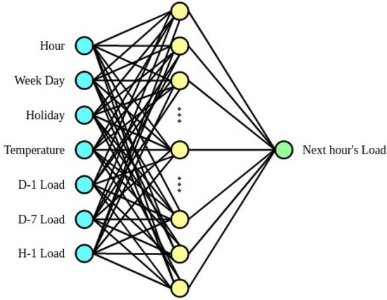
Figure 1.
The structure of the proposed MLP neural network.
3. Results
The pre-processing techniques for the data input to the neural network are of particular interest when developing the current prediction model. The MSE, MAE and MAPE metrics are used to assess and compare the various scaling methods for the input data.
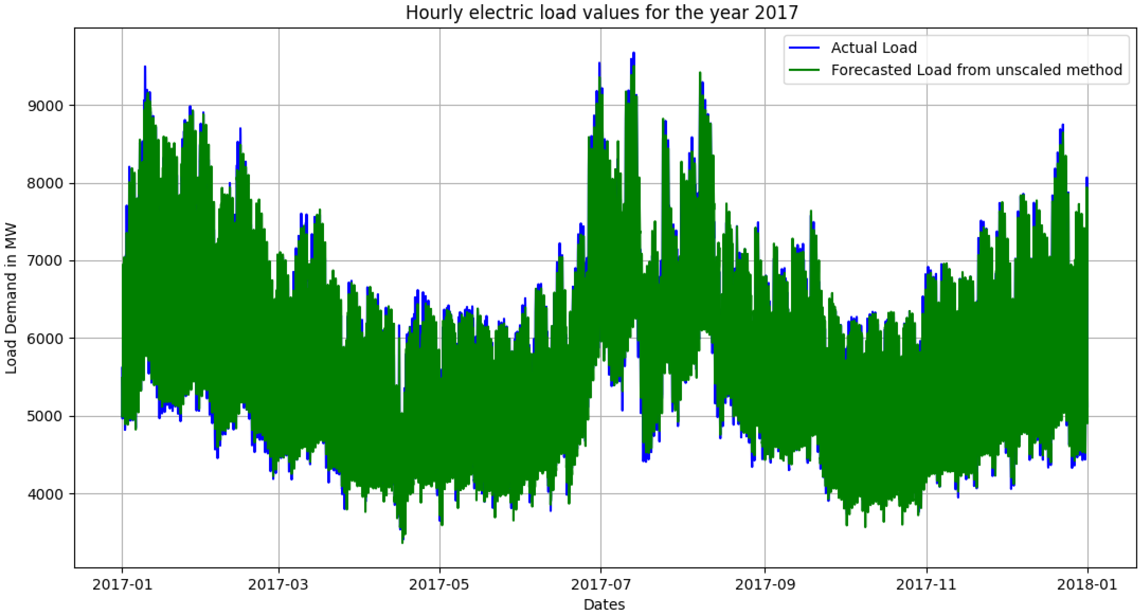
Initially the input data are not subjected to some kind of processing and are entered into the three-layer perceptron in the original form of raw data. The results of this method are compared to the real hourly load values for the respective day for the entire year of 2017. The real and forecasted values are graphically depicted in Figure 2, while the values for the metric indicators are summarized in Table 1.

Figure 2.
Graphic comparison of actual and predicted hourly load values without any pre-processing of the data.

Table 1.
MSE, MAE and MAPE values for the hourly load forecast. Input data are not subjected to any scaling technique.
Next, the effect of a simple scaling of the input data on the prediction result of the neural network is studied. Simple scaling is performed by dividing each input variable by the maximum value of the corresponding dataset. This procedure is performed only for the , , and variables in order to obtain values within the field [0, 1]. Equation (1) gives the simple scaling for the temperature:
where is the hourly temperature value of ith day and is the maximum hourly temperature value of the dataset. The , and data are normalized in a similar way.
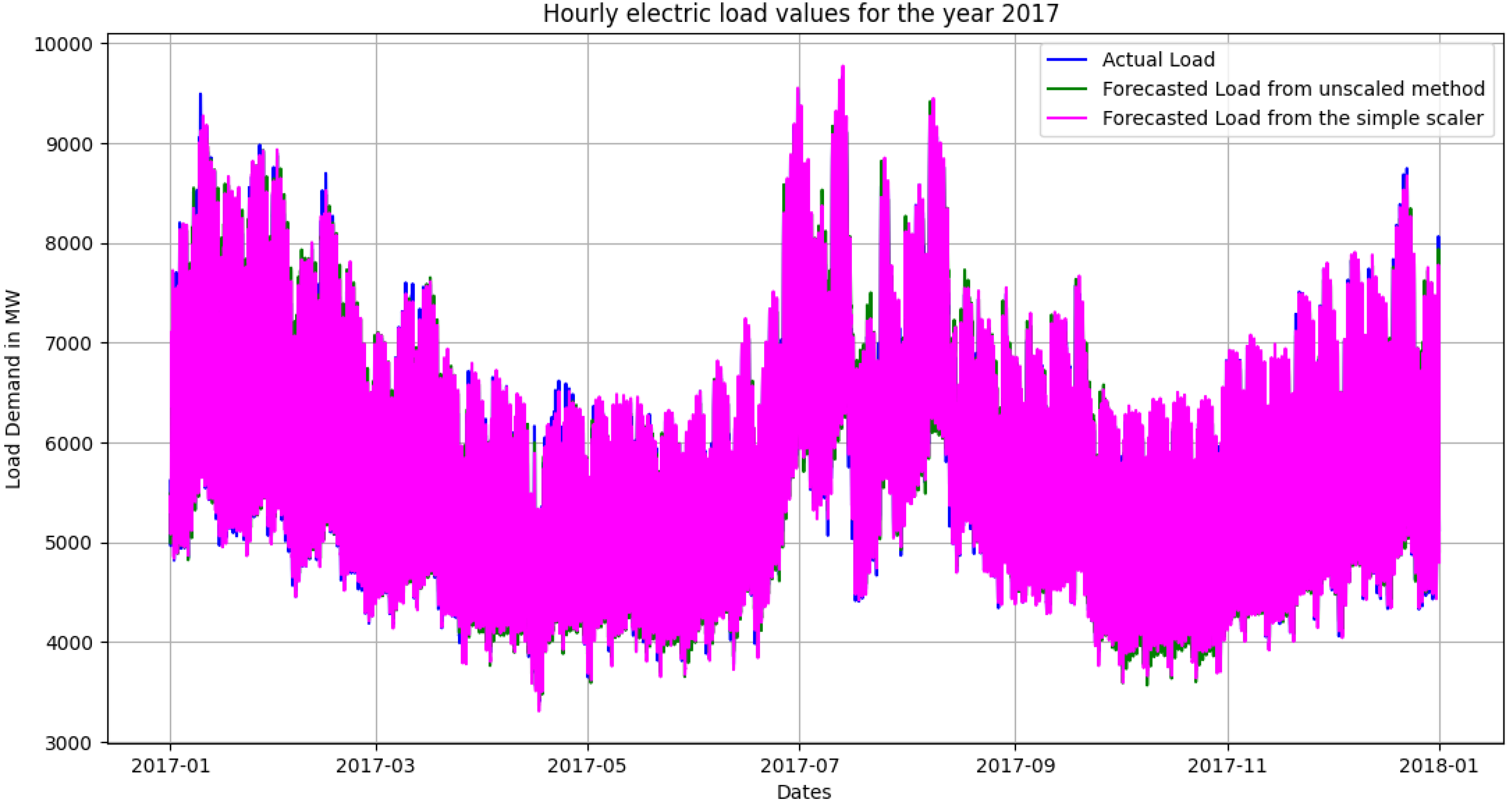
The scaled data are then fed into a neural network, which predicts the load’s hourly value. The results of the proposed neural network are compared to real-time hourly values from 2017. Figure 3 depicts its graphic display. The MSE, MAE, and MAPE metrics calculated from this forecast using the same input data pre-processing technique are summarized in Table 2.
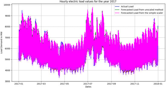
Figure 3.
Graphic comparison of actual and predicted hourly load values for the year 2017. The values predicted through the simple scaling method are added.
Table 2.
MSE, MAE and MAPE values for the hourly load forecast. Input data are subjected to a simple scaling technique.
After an extensive study of the correlation of the data, and the way in which the neural network manages them, this work proposed an innovative scaling method that will provide appropriate weight to the variables , and , thereby considerably improving the forecast results.
First, temperature data are scaled in the same way as in discussed above, using Equation (1). After experimentation, it was observed that the , and data determine, to a greater extent, the outcome of the neural network. Therefore, it is considered reasonable and necessary to give them due consideration and as a result of experimentation the coefficient 10 is the appropriate weight for these variables. The proposed scaling technique is described by Equation (2):
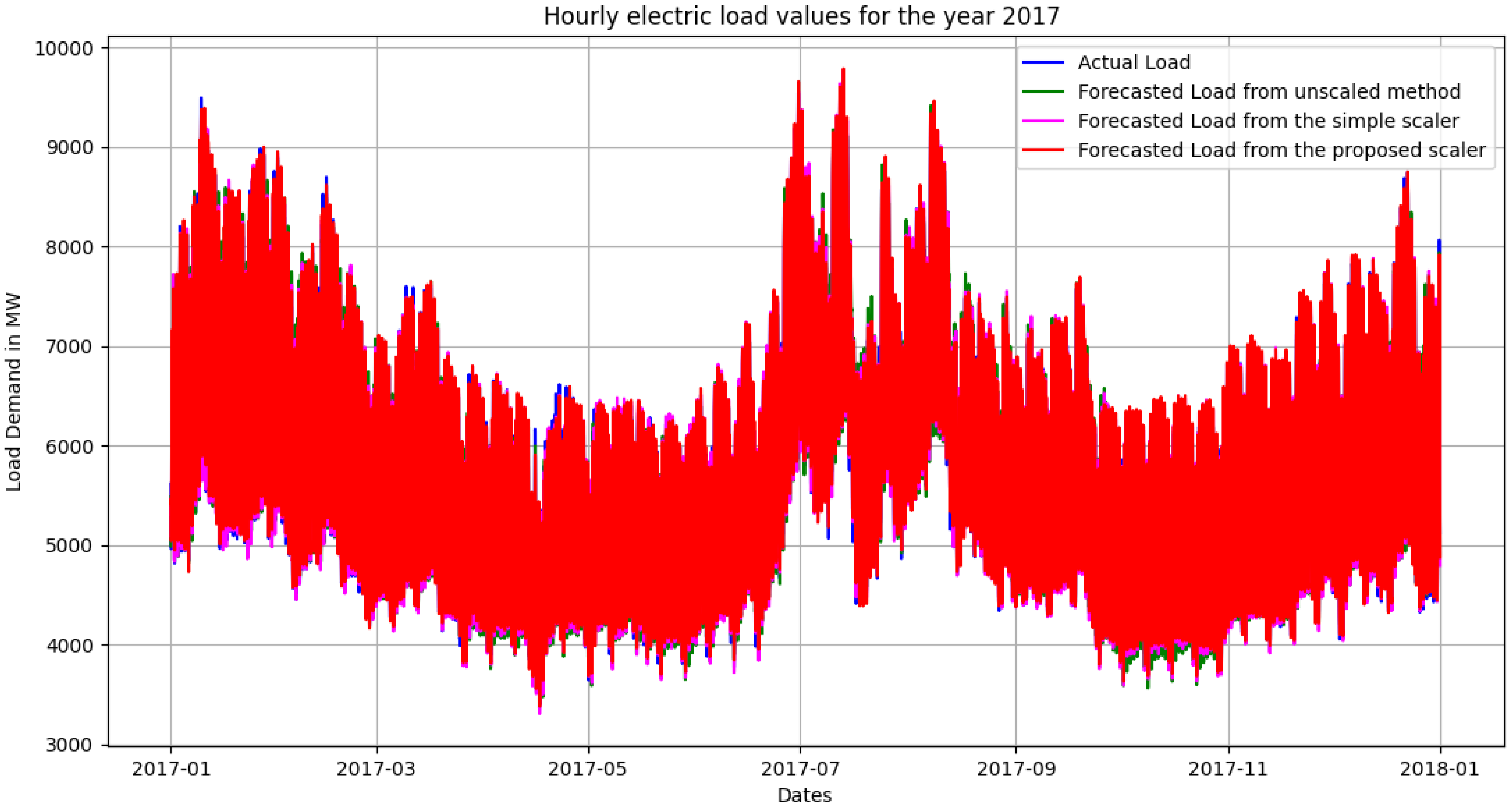
Second, the scaled data are fed into the neural network. Figure 4 graphically depicts the resulting outcomes, which correspond to real and predicted hourly values for the year 2017. The MSE, MAE, and MAPE values calculated from this forecast are compared in Table 3. Our proposed data pre-processing technique significantly improves forecasting, so the MAPE values fall.

Figure 4.
Graphic comparison of actual and predicted hourly load values for the year 2017. The values predicted through the proposed scaling method are added.
Table 3.
MSE, MAE and MAPE values for the hourly load forecast. Input data is subjected to enhanced scaling technique.
The Min–Max method is a popular way of scaling neural network input data for regression problems. The temperature data and historical load data are subjected to a separate Min–Max scaling, as Equation (3) shows:
where y is the new scaled value, x is the initial value, and are the minimum and maximum values of the set, respectively.
The scaled data will now be inserted into the input layer to predict hourly load values for the year 2017. As shown in Figure 5, the values of the forecast results using the proposed MLP neural network are graphically compared to the real values. The values of the estimated MSE, MAE, and MAPE metrics are summarized in Table 4.

Figure 5.
Graphic comparison of actual and predicted hourly load values for the year 2017. The values predicted through the min–max scaling method are added.
Table 4.
MSE, MAE and MAPE values for the hourly load forecast. Input data are subjected to a min–max scaling technique.
While Min–Max scaling does not seem to do as well as the other two data pre-processing methods, an improved Min–Max Scaling approach that stresses the value and weight of input variables and in the forecast outcome should also be considered. The temperature data are first scaled using the basic min–max equation, while the historical load data are scaled using Equation (4):
where y represents the current scaled value, x represents the load’s hourly value, and and represent the minimum and maximum values of all historical load results, respectively. The variables and get values in the field [0, 10] using Equation (4).
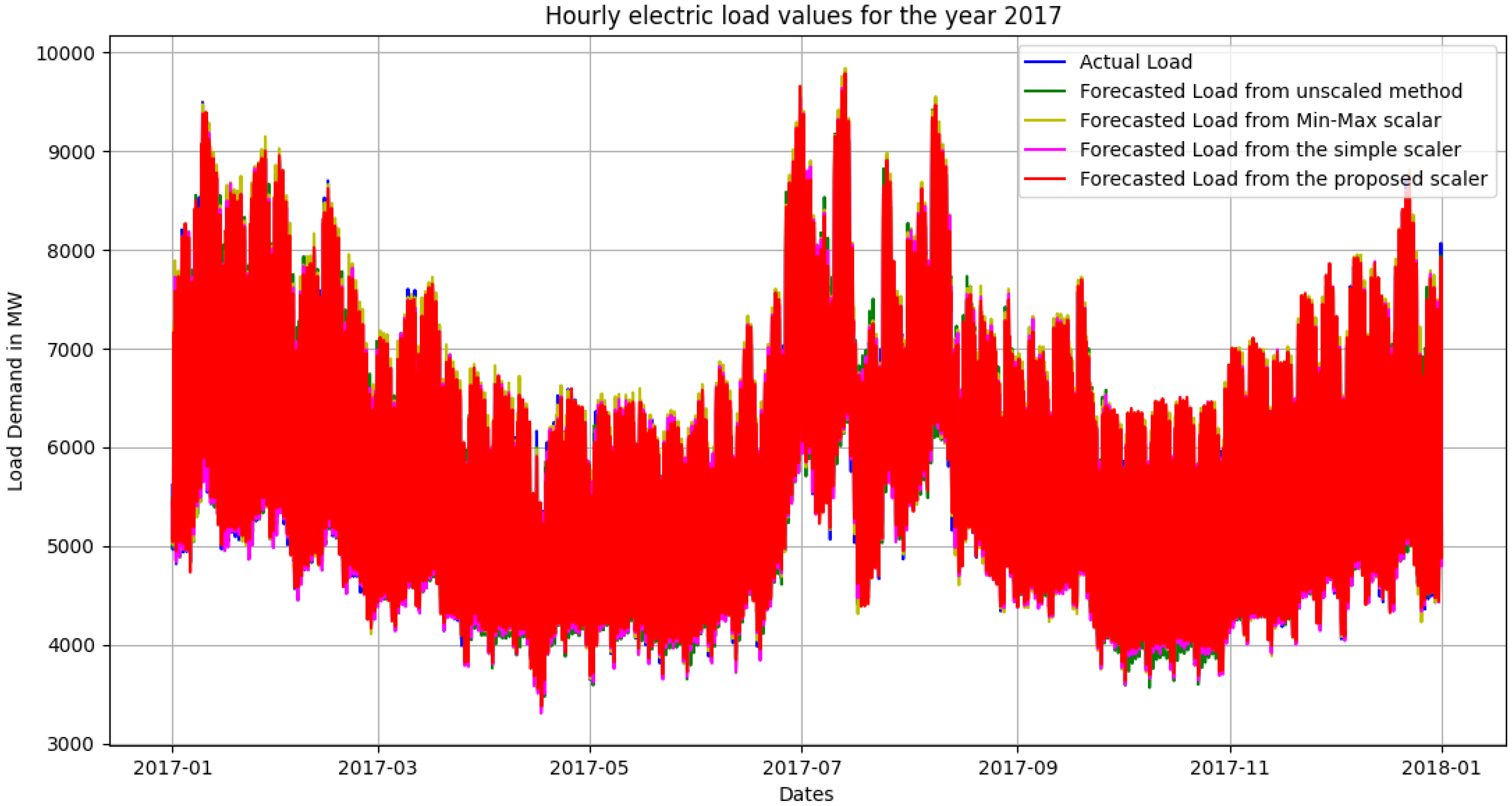
The data have now been scaled and entered into the proposed neural network. The forecast’s outcome is a value in the interval [0, 10] that corresponds to the day’s hourly load on which the forecast is conducted. This value can be translated to MW so that it can be compared to the corresponding real hourly load value and the MSE, MAE, and MAPE metrics can be correctly calculated. Equation (5) is used to convert this value to MW. The load behaviour of all scaling methods evaluated is depicted in Figure 6.
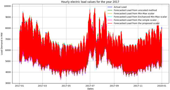
Figure 6.
Graphic comparison of actual and predicted hourly load values for the year 2017. All pre-processing methods of the examined data are illustrated graphically.
The results of the MSE, MAE, and MAPE metrics are summarized in Table 5, which serve as a reference point for all scaling approaches for the hourly load forecast for 2017.
Table 5.
MSE, MAE and MAPE values for the hourly load forecast. The metrics for each scaling approach investigated are aggregated.
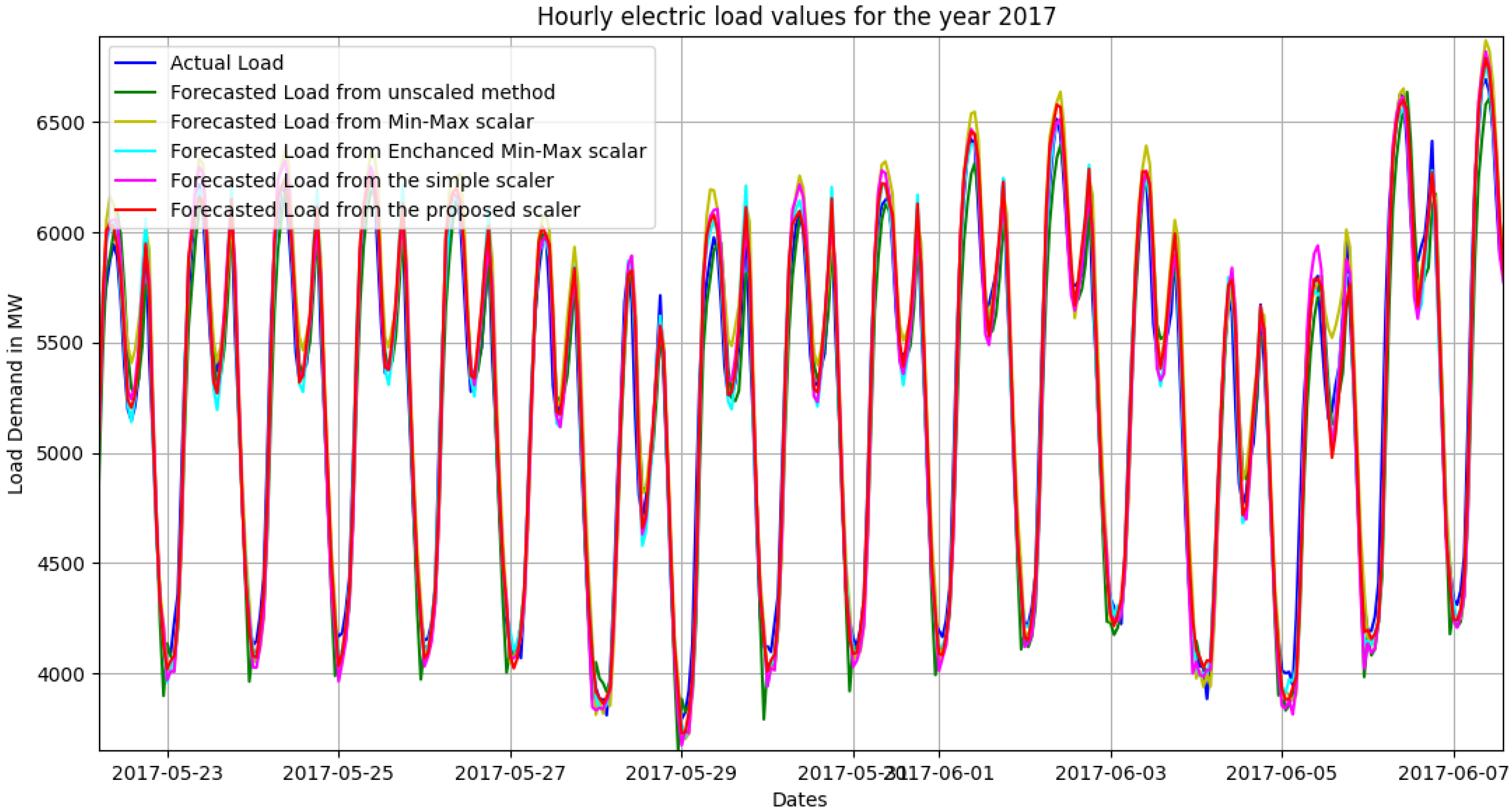
Our improved Min–Max Scaling strateg produces a lower MAPE value in the prediction. In terms of MLP performance, this approach sufficiently stresses the weight and value of the input variables , , and , despite its relative simplicity. It is worth noting that when this improved MLP neural network is combined with our proposed enhanced scaling approach, the MAPE value drops below 2%, resulting in the lowest prediction value in the literature, based on data from the Greek interconnected power system. Figure 7 and Figure 8 show the value of the weight attached to the input data in greater detail.

Figure 7.
The various load curves for 2 weeks of 2017. The proposed method effectively follows the actual load curve.

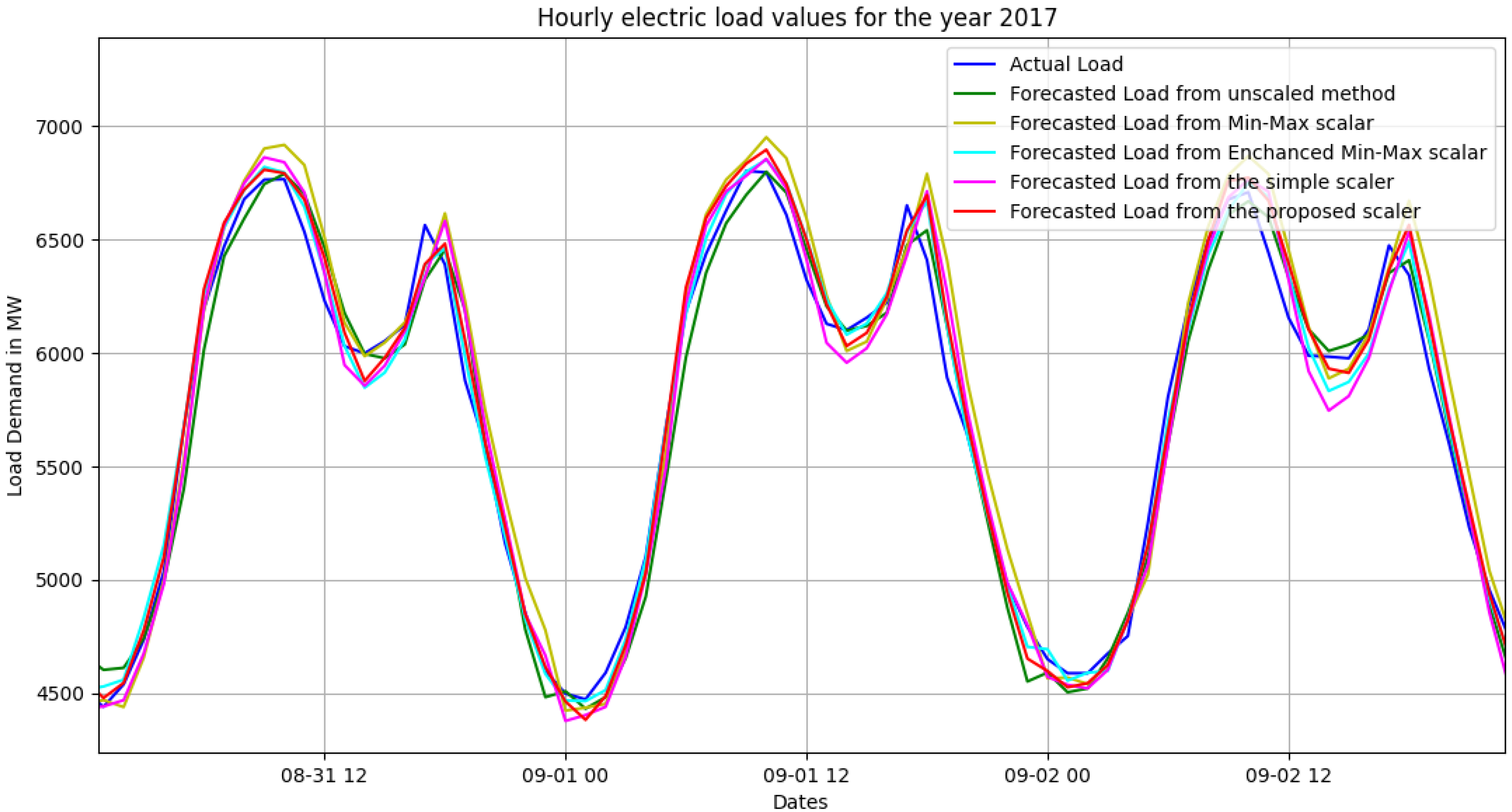
Figure 8.
A more detailed depiction of the various load curves.
4. Discussion
Short-term load forecasting is a growing area of study, in which interest is expected to increase in coming years, as its outcomes impact virtually all aspects of the management and operation of a power system. Modelling, identification and performance analysis are all used in the development of statistical load forecasting models. Computational intelligence approaches are expected to be the driving force behind this field, because they enable the generalization and simulation of non-linear dynamic systems.
Most STLF approaches employ neural networks of various kinds. In this work, we developed an MLP and trained it using data from the Greek electricity system, thus contributing to the literature on the application of ANNs to STLF in general, and to the special case of the application of ANNs to the Greek electricity system. Moreover, it has been demonstrated in the literature, and shown in this paper, that the accuracy of the predictions achieved by the neural network can be greatly improved, if some kind of pre-processing is applied to the input data [6,15] or if the output of the neural network is post-processed [35]. There are also approaches that exploit correlations between input data to improve the prediction performance of the neural network [36,37].
In this paper, we use historical load data, in contrast to approaches such as the one in [37], and couple this with data pre-processing methods, in contrast to approaches such as [35], rather than post-processing the output of the neural network. We show that the simple scaling of input through normalization, such as the one proposed in [6], can be further improved through our proposal for enhanced scaling, where the importance of certain input variables on the total outcome of the neural network is taken into consideration. Moreover, we propose an improvement to the Min–Max normalization used by [15] by implementing enhanced Min–Max scaling, and demonstrate that the accuracy of the prediction produced by the MLP is further increased. Hence, the overall prediction performance of the MLP is significantly better when our proposed data pre-processing techniques are applied, while the neural network maintains its simplicity, yielding MAPE values below 2%.
Despite the simplicity of the MLP model described in our study, the obtained MAPE results are more accurate than those produced by the complicated approaches presented in [28,29]. Furthermore, when compared to [29], where a new way of scaling input data is utilized, the results of our study are more accurate, highlighting the effectiveness of the suggested scaling approach. The presented scaling technique in our study outperforms [30,31], underlining the necessity of assigning more importance to specific input data.
Our future work will focus on investigating whether the coefficients we used for the weighted enhancements on data pre-processing can be calculated in some formal manner, rather than empirically derived. We also intend to study the impact of various clustering techniques on the prediction performance, in order to compare our approach with the works in [11,14].
Author Contributions
Conceptualization, A.I.A.; methodology, A.I.A.; software, A.I.A.; validation, A.I.A., D.B. and A.D.; formal analysis, A.I.A.; investigation, A.I.A.; resources, A.I.A. and V.M.L.; data curation, A.I.A. and V.M.L.; writing—original draft preparation, A.I.A.; writing—review and editing, A.I.A., D.B., A.D. and L.H.T.; visualization, A.I.A. and V.M.L.; supervision, D.B., A.D. and L.H.T.; project administration, D.B., A.D. and L.H.T. All authors have read and agreed to the published version of the manuscript.
Funding
This research received no external funding.
Institutional Review Board Statement
Not applicable.
Informed Consent Statement
Not applicable.
Data Availability Statement
Data are available in a publicly accessible repository. The data used in this study are openly available from the Greek Regulatory Authority (REA) in https://open-power-system-data.org/data-sources (accessed on 5 February 2021). The dataset was processed as the input for the design and performance assessment of the multi-layer perceptron neural network described in this article.
Conflicts of Interest
The authors declare no conflict of interest.
References
- Ongsakul, W.; Dieu, V.N. Artificial Intelligence in Power System Optimization; CRC Press, Inc.: Boca Raton, FL, USA, 2013. [Google Scholar]
- Kyriakides, E.; Polycarpou, M. Short Term Electric Load Forecasting: A Tutorial. In Trends in Neural Computation; Chen, K., Wang, L., Eds.; Springer: Berlin/Heidelberg, Germany, 2007; pp. 391–418. [Google Scholar] [CrossRef]
- Metaxiotis, K.; Kagiannas, A.; Askounis, D.; Psarras, J. Artificial intelligence in short term electric load forecasting: A state-of-the-art survey for the researcher. Energy Convers. Manag. 2003, 44, 1525–1534. [Google Scholar] [CrossRef]
- Alamaniotis, M.; Bargiotas, D.; Tsoukalas, L. Towards Smart Energy Systems: Application of Kernel Machine Regression for Medium Term Electricity Load Forecasting. SpringerPlus 2016, 5, 58. [Google Scholar] [CrossRef] [PubMed] [Green Version]
- Kontogiannis, D.; Bargiotas, D.; Daskalopulu, A. Fuzzy Control System for Smart Energy Management in Residential Buildings Based on Environmental Data. Energies 2021, 14, 752. [Google Scholar] [CrossRef]
- Alamaniotis, M.; Ikonomopoulos, A.; Alamaniotis, A.; Bargiotas, D.; Tsoukalas, L.H. Day-ahead electricity price forecasting using optimized multiple-regression of relevance vector machines. In Proceedings of the 8th Mediterranean Conference on Power Generation, Transmission, Distribution and Energy Conversion (MEDPOWER 2012), Cagliari, Italy, 1–3 October 2012; pp. 1–5. [Google Scholar] [CrossRef]
- Alamaniotis, M.; Bargiotas, D.; Bourbakis, N.G.; Tsoukalas, L.H. Genetic Optimal Regression of Relevance Vector Machines for Electricity Pricing Signal Forecasting in Smart Grids. IEEE Trans. Smart Grid 2015, 6, 2997–3005. [Google Scholar] [CrossRef]
- Park, D.; El-Sharkawi, M.; Marks, R.; Atlas, L.; Damborg, M. Electric load forecasting using an artificial neural network. IEEE Trans. Power Syst. 1991, 6, 442–449. [Google Scholar] [CrossRef] [Green Version]
- Ho, K.; Hsu, Y.Y.; Yang, C.C. Short term load forecasting using a multilayer neural network with an adaptive learning algorithm. IEEE Trans. Power Syst. 1992, 7, 141–149. [Google Scholar] [CrossRef]
- Peng, T.; Hubele, N.; Karady, G. Advancement in the application of neural networks for short-term load forecasting. IEEE Trans. Power Syst. 1992, 7, 250–257. [Google Scholar] [CrossRef]
- Kandil, N.; Wamkeue, R.; Saad, M.; Georges, S. An efficient approach for short term load forecasting using artificial neural networks. Int. J. Electr. Power Energy Syst. 2006, 28, 525–530. [Google Scholar] [CrossRef]
- Bakirtzis, A.; Petridis, V.; Kiartzis, S.; Alexiadis, M.; Maissis, A. A neural network short term load forecasting model for the Greek power system. IEEE Trans. Power Syst. 1996, 11, 858–863. [Google Scholar] [CrossRef]
- Mandal, P.; Senjyu, T.; Funabashi, T. Neural networks approach to forecast several hour ahead electricity prices and loads in deregulated market. Energy Convers. Manag. 2006, 47, 2128–2142. [Google Scholar] [CrossRef]
- Tsekouras, G.; Kanellos, F.; Kontargyri, V.; Karanasiou, I.; Elias, C.; Salis, A.; Mastorakis, N. A Comparison of Artificial Neural Networks Algorithms for Short Term Load Forecasting in Greek Intercontinental Power System. 2008. Available online: http://users.ntua.gr/vkont/CSECS_2008.pdf (accessed on 5 February 2021).
- Alamaniotis, M.; Tsoukalas, L.H. Anticipation of minutes-ahead household active power consumption using Gaussian processes. In Proceedings of the 2015 6th International Conference on Information, Intelligence, Systems and Applications (IISA), Corfu, Greece, 6–8 July 2015; pp. 1–6. [Google Scholar] [CrossRef]
- Kontogiannis, D.; Bargiotas, D.; Daskalopulu, A. Minutely Active Power Forecasting Models Using Neural Networks. Sustainability 2020, 12, 3177. [Google Scholar] [CrossRef] [Green Version]
- Yun, Z.; Quan, Z.; Caixin, S.; Shaolan, L.; Yuming, L.; Yang, S. RBF Neural Network and ANFIS-Based Short-Term Load Forecasting Approach in Real-Time Price Environment. IEEE Trans. Power Syst. 2008, 23, 853–858. [Google Scholar] [CrossRef]
- Chang, W.Y. Short-Term Load Forecasting Using Radial Basis Function Neural Network. J. Comput. Commun. 2015, 3, 40–45. [Google Scholar] [CrossRef] [Green Version]
- Cecati, C.; Kolbusz, J.; Różycki, P.; Siano, P.; Wilamowski, B.M. A Novel RBF Training Algorithm for Short-Term Electric Load Forecasting and Comparative Studies. IEEE Trans. Ind. Electron. 2015, 62, 6519–6529. [Google Scholar] [CrossRef]
- Hanmandlu, M.; Chauhan, B.K. Load Forecasting Using Hybrid Models. IEEE Trans. Power Syst. 2011, 26, 20–29. [Google Scholar] [CrossRef]
- Panapakidis, I.P. Clustering based day-ahead and hour-ahead bus load forecasting models. Int. J. Electr. Power Energy Syst. 2016, 80, 171–178. [Google Scholar] [CrossRef]
- Dong, X.; Qian, L.; Huang, L. Short-term load forecasting in smart grid: A combined CNN and K-means clustering approach. In Proceedings of the 2017 IEEE International Conference on Big Data and Smart Computing (BigComp), Jeju, Korea, 13–16 February 2017; pp. 119–125. [Google Scholar] [CrossRef]
- Amjady, N.; Keynia, F. A New Neural Network Approach to Short Term Load Forecasting of Electrical Power Systems. Energies 2011, 4, 488–503. [Google Scholar] [CrossRef]
- Ekonomou, L.; Christodoulou, C.; Mladenov, V. A short-term load forecasting method using artificial neural networks and wavelet analysis. Int. J. Power Syst. 2016, 1, 64–68. [Google Scholar]
- Fahiman, F.; Erfani, S.M.; Rajasegarar, S.; Palaniswami, M.; Leckie, C. Improving load forecasting based on deep learning and K-shape clustering. In Proceedings of the 2017 International Joint Conference on Neural Networks (IJCNN), Anchorage, AK, USA, 14–19 May 2017; pp. 4134–4141. [Google Scholar] [CrossRef]
- Liu, N.; Tang, Q.; Zhang, J.; Fan, W.; Liu, J. A hybrid forecasting model with parameter optimization for short-term load forecasting of micro-grids. Appl. Energy 2014, 129, 336–345. [Google Scholar] [CrossRef]
- Aly, H.H. A proposed intelligent short-term load forecasting hybrid models of ANN, WNN and KF based on clustering techniques for smart grid. Electr. Power Syst. Res. 2020, 182, 106191. [Google Scholar] [CrossRef]
- Massaoudi, M.; Refaat, S.S.; Chihi, I.; Trabelsi, M.; Oueslati, F.; Abu-Rub, H. A novel stacked generalization ensemble-based hybrid LGBM-XGB-MLP model for Short-Term Load Forecasting. Energy 2020, 214, 118874. [Google Scholar] [CrossRef]
- Syed, D.; Abu-Rub, H.; Ghrayeb, A.; Refaat, S.S.; Houchati, M.; Bouhali, O.; Bañales, S. Deep Learning-Based Short-Term Load Forecasting Approach in Smart Grid With Clustering and Consumption Pattern Recognition. IEEE Access 2021, 9, 54992–55008. [Google Scholar] [CrossRef]
- Wu, L.; Kong, C.; Hao, X.; Chen, W. A Short-Term Load Forecasting Method Based on GRU-CNN Hybrid Neural Network Model. Math. Probl. Eng. 2020, 2020, 1–10. [Google Scholar] [CrossRef] [Green Version]
- Farsi, B.; Amayri, M.; Bouguila, N.; Eicker, U. On Short-Term Load Forecasting Using Machine Learning Techniques and a Novel Parallel Deep LSTM-CNN Approach. IEEE Access 2021, 9, 31191–31212. [Google Scholar] [CrossRef]
- Hossen, T.; Plathottam, S.J.; Angamuthu, R.K.; Ranganathan, P.; Salehfar, H. Short-term load forecasting using deep neural networks (DNN). In Proceedings of the 2017 North American Power Symposium (NAPS), Morgantown, WV, USA, 17–19 September 2017; pp. 1–6. [Google Scholar] [CrossRef]
- Raza, M.Q.; Khosravi, A. A review on artificial intelligence based load demand forecasting techniques for smart grid and buildings. Renew. Sustain. Energy Rev. 2015, 50, 1352–1372. [Google Scholar] [CrossRef]
- Ryu, S.; Noh, J.; Kim, H. Deep neural network based demand side short term load forecasting. In Proceedings of the 2016 IEEE International Conference on Smart Grid Communications (SmartGridComm), Sydney, Australia, 6–9 November 2016; pp. 308–313. [Google Scholar] [CrossRef]
- Zhu, J. Optimization of Power System Operation; IEEE: Piscataway, NJ, USA, 2015; p. 623. [Google Scholar] [CrossRef]
- Singh, H.; Lone, Y.A. Artificial Neural Networks. In Deep Neuro-Fuzzy Systems with Python: With Case Studies and Applications from the Industry; Apress: Berkeley, CA, USA, 2020; pp. 157–198. [Google Scholar] [CrossRef]
- Twomey, J.; Smith, A. Performance measures, consistency, and power for artificial neural network models. Math. Comput. Model. 1995, 21, 243–258. [Google Scholar] [CrossRef]

Publisher’s Note: MDPI stays neutral with regard to jurisdictional claims in published maps and institutional affiliations. |
© 2021 by the authors. Licensee MDPI, Basel, Switzerland. This article is an open access article distributed under the terms and conditions of the Creative Commons Attribution (CC BY) license (https://creativecommons.org/licenses/by/4.0/).