Abstract
This study investigates the relative role of land surface schemes (LSS) in the Weather Research and Forecasting (WRF) model, Version 4, to simulate the heat wave events in Karachi, Pakistan during 16–23 May 2018. The efficiency of the WRF model was evaluated in forecasting heat wave events over Karachi using the three different LSS, namely NOAH, NOAH-MP, and RUC. In addition to this we have used the longwave (RRTM) and shortwave (Dudhia) in all schemes. Three simulating setups were designed with a combination of shortwave, longwave, and LSS: E1 (Dudhia, RRTM, and Noah), E2 (Dudhia, RRTM, and Noah-MP), and E3 (Dudhia, RRTM, and RUC). All setups were carried out with a finer resolution of 1 km × 1 km. Findings of current study depicted that E2 produces a more realistic simulation of daily maximum temperature T(max) at 2 m, sensible heat (SH), and latent heat (LH) because it has higher R2 and lower errors (BIAS, RMSE, MAE) compared to other schemes. Consequently, Noah-MP (LSS) accurately estimates T(max) and land surface heat fluxes (SH&LH) because uses multiple physics options for land atmosphere interaction processes. According to statistical analyses, E2 setup outperforms other setups in term of T(max) and (LH&SH) forecasting with the higher Nash-Sutcliffe efficiency (NSE) agreement is 0.84 (0.89). This research emphasizes that the selection of LSS is of vital importance in the best simulation of T(max) and SH (LH) over Karachi. Further, it is resulted that the SH flux is taking a higher part to trigger the heat wave event intensity during May 2018 due to dense urban canopy and less vegetated area. El Niño-Southern Oscillation (ENSO) event played role to prolong and strengthen the heat wave period by effecting the Indian Ocean Dipole (IOD) through walker circulation extension.
1. Introduction
Extreme climate events have gained a lot of attention due to their significant environmental and societal impacts [1]. Anthropogenic activities including deforestation and high fossil fuel consumption, stimulate the emission of greenhouse gases which in turns play an important roles in changes of climatology of Earth System. Heat waves are one of the world’s most serious climate threats with their subtle environmental consequences [2]. Besides, the extreme temperature is significantly increasing evaporation rate, which eventually resulting in dry spells [3,4]. For example, an average temperature in the Loess Plateau, China has been increased in recent decades, indicating that extreme weather patterns are becoming more common as a result of global warming [5]. Karachi, Pakistan is particularly vulnerable to the climate change scenarios like as extreme heat, drought, and sea level rise.
Heat waves are identified as an irregular period of hot or humid weather that is persisting for three to five consecutive days during the summer. The World Meteorological Organization’s (WMO) definition of a heat wave is as follows: “A heat wave occurs when the daily maximum temperature T(max) for more than five consecutive days exceeds the average maximum temperature by 5 °C” [6]. Some studies reported that the occurrence and intensity of heat waves have increased globally in past few years [7]. The 18-year variation of T(max) during the May is presented in Figure 1.
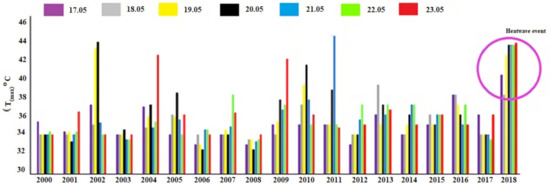
Figure 1.
Temporal variation of T(max) during May (2000–2018). Data is collected from the climate station Karachi, Pakistan. Color shows different days.
Pakistan is densely populated country with more than 200 million people and is extremely vulnerable to climate change. In June 2015, Pakistan endured a deadliest heat wave in Karachi, with over 1300 people dying. Heat waves have a significant impact on Pakistan’s urban and rural areas, as well as economic indicators such as livestock, agriculture, and people [8]. Zhaid and Rasul (2010) reported that climatology of summer season has changed by an increase in 6.2% of humidity and 0.25 °C of T(max) from 1961–2017 over the Pakistan which in turn has increased the magnitude of heat waves in past several years [9].
Regional climate models (RCMs) are used all around the world to extract fine-scale climate data from the global climate models (GCM) [10]. RCMs can resolve better mesoscale phenomena linked with a local climate such as temperature and precipitation systems due to improved surface physics and high resolution [11,12]. Numerical weather prediction models (NWP) models were used to study the mechanism for heat wave and investigate the land-atmosphere interactions [13,14,15]. The current advancement to run the NWP models with high computation power and frequency input data has enable it to forecast the heat wave events with a fine resolution over a large scale. In recent years, the forecasting capability of NWP models has improved that encouraging the researcher their use to simulate weather parameters at a high spatial and temporal resolution for research and operational purposes. WRF model is a state-of-the-art RCM for dynamic downscaling [16]. However, accurate implementation of NWP models to predict the heat wave events and other climatology required a careful selection of model parameterization schemes [17]. In the NWP model, various physical parameterization schemes are used to predict weather forecasts [18]. Therefore, selecting a proper combination of physical parameterization schemes is very extremely important as it strongly affects simulation [15].
Land surface processes have a significant impact on high temperatures. Land surface consists of complex and variant surfaces that are very vital part of the atmosphere boundary. The exchange of energy, water vapor, momentum, and radiative transfer between the land and atmosphere is controlled by land surface processes. Therefore, there is very close relationship between the land surface and high temperature that affect local, regional, and global atmospheric circulation as well as climate change [19]. Reviewing the previous studies, the sensitivity of four LSS in the WRF, namely the simple soil thermal diffusion (STD) scheme, Noah scheme, RUC scheme, and community land model was investigated by Jin, Miller et al. (2010). Their finding reveal that land surface activities have a significant impact on temperature simulations in western United States [20]. Lhotka, Kyselý et al. (2018) studied the performance of model in simulating the land-atmosphere interactions and large-scale circulation associated with heat waves using RCMs. It was concluded that the RCMs overestimated and underestimated the events over the central Europe while the ensemble mean of EURO-CORDEX captures the heat wave extremity index well [21].
Zeng, Wu et al. (2011) concluded that sensitivity of simulation of high temperature to different LSS in East China is higher for the medium timescale forecast. Also, the change in high temperature is consistent with change in SH [22]. Zittis and Hadjinicolaou (2017) quantified the sensitivity of the WRF model to short and long wave radiation schemes by choosing two scheme and concluded that performance of radiation scheme is depending on the season, location, and land use type [23]. Zittis, Hadjinicolaou et al. (2014) analyzed the performance of different physics schemes by testing combination with the cumulus, planetary boundary layer, and micro physics schemes in the WRF and revealed that cloud microphysics scheme has strong impact on temperature particularly in the tropics [24].
Bucchihnani, Cattaneo et al. (2016) investigated the performance of COSMO-CLM related to convection, radiation, surface, and cloud parameterization schemes, showing that incorporating new schemes of albedo and aerosols, the model showed mean absolute error 15 mm/month for rainfall and 1.2 °C for temperature [25]. Constantinidou, Hadjinicolaou et al. (2020) simulated the climate over the Middle East North Africa (MENA) region using WRF model and tested four different LSS in six numerical experiments [26]. Davin, Maisonnave et al. (2016) revealed the effect of LSS on summer temperature modelled over southern Europe [27]. Recently, different models explored the impact of LSS on climate simulation over EURO-CORDEX, and CORDEX-Africa [28,29]. Sun, Hu et al. (2018) studied the heat wave severity in China using Canadian Earth System Model Version 2 (CanESM2) and found that the global warming associated with severe heat waves including longer heat wave season, higher hottest day temperature, and more heat wave days [30]. Mortezazadeh, Jandaghian al. (2021) applied the WRF model to investigate the role of metrological processes on the temperature during the heat wave event in 2017 and concluded that a difference of 4 ms−1 wind speed might result in temperature changes of 4 °C [31]. The WRF is a globally used NWP model for analyzing atmospheric processes and extreme weather conditions such as cold waves, heat waves, and precipitation [32]. Tian and Miao (2019) simulated mountain plain breeze circulation using BouLac PBL (planetary boundary layer), Noah + UCM land surface, and MM5 surface layer schemes in the WRF model in eastern Chengdu, China [33]. Mohan and Gupta (2018); Gunwani and Mohan (2017); Sathyanadh, Prabha et al. (2017) simulated the meteorological variables using the number of physical WRF schemes in various parts of India to boost the WRF results [34,35,36]. In the Iran region, the effect of 26 various PBL, cumulus, and microphysical schemes on summer rainfall was investigated [37]. The sensitivity schemes of the WRF model were checked with a different combination of microphysics schemes across northwest India, and revealed that a combination of physical parameterization schemes such as Kain-Fritsch cumulus, YSU PBL, Dudhia shortwave, RRTM longwave radiation, and one-moment microphysics schemes reproduced better results from the WRF model [32]. Sahoo, Ajilesh et al. (2020) used the WRF physics options WSM6 scheme, Dudhia shortwave, RRTM longwave, cumulus New Kain-Fritsch scheme, YSU PBL scheme, and Noah surface model to simulate extreme rainfall in various sensitivity experiments over Uttarakhand region of India [38]. The physical parameterization schemes of the WRF model were evaluated forsimulation of the rainfall event on Tamil Nadu, India’s northeast coast and resulted that rainfall events in Tamil Nadu, India can be better simulated by combining YSU PBL, Noah LSM, and Goddard microphysics schemes [39]. A study in the Bay of Bengal explored the best scheme by simulating extreme cyclonic storm with WRF model and resulted that the Ferrier scheme provided the best forecast of the cyclone [40]. Similarly, Choudhury, and Das (2017) investigated the sensitivity of the WRF model to simulate the strength and track of cyclones and concluded that Thompson and Goddard schemes better predicted the cyclone strength [41]. The ability of the WRF model prediction with different microphysics schemes was investigated to simulate the frequency of precipitation in western Nepal and suggested that the Thompson microphysics scheme is better to simulate convective events of rainfall [42]. The WRF model employs multiple parameterization schemes such as clouds, turbulence, heat, surface, and cumulus convection are used to predict weather forecasts [18]. The WRF model simulations are quite sensitive to the selection of combination of physics schemes, and it includes several options for parameterizing surface layer microphysics, cumulus parameterization, PBL, ground surface, and clouds.
The inter-annual changes in summer heatwaves at a shorter period are significantly linked with modes of climate variability. For example, heatwaves in eastern and southern China is modulated by the westward extension of the western North Pacific (WNP) subtropical [43,44]. The ENSO, an important scale phenomena with significant impacts on the mean seasonal climate around the world [45,46]. Heatwaves are prominently affected by the ENSO variability in many parts of the world such as East Asia, Southeast Asia, Australia, Canada, and America [47,48,49,50,51,52]. Luo and Lau (2019) found that the heatwaves in southern and eastern China experienced intensive heatwaves during summer due to decaying El Nino [53].
The region of Karachi, Pakistan is historically exposed to increasing heatwave and extreme precipitation that have been increasing in the past and more enhancing in the 21 century. Research on how the model physics influences the simulated climate in the Pakistan region has been still unknown. It is important to investigate extreme events occurrences using numerical weather forecasting skills through the WRF model. There are no such studies before on the assessment of WRF model sensitivity to LSS over the Karachi node, Pakistan. Therefore, the impact of different WRF LSS on heat wave event is study of importance. It can be beneficial to be responsive and adaptable to hazards in the future. The Noah and RUC schemes are at average level of complexity, but RUC scheme has relativity more complex snow scheme. Noah-MP includes the snow depth, surface radiation balance, heat fluxes, vegetation, and canopy temperature difference and runoff etc. The principal objective of present study is evaluating the role of LSS in the simulation of heat wave by choosing different LSS including Noah, Noah-MP, and RUC in WRF model over Karachi, Pakistan. Evaluate the role of LSS coupled with WRF model can lead to a better understanding of heatwave events and how land surface processes affect the regional climate. In particular, we investigate how ocean-land circulations prolong and strengthen the heat wave and tried explaining some reasons. Current study area is very attractive for its worth as major node area in the Belt and Road Initiative (BRI) Project with sharp climatic gradients.
2. Materials and Methods
2.1. Study Area
The study focuses on the Karachi city in Pakistan, located between 24.8607° N, 67.0011° E shown in Figure 2. The study area covers 3780 km2, with an altitude of 10 m above sea level. It has scattered rocky outcrops, coastal marshlands, and mountains. Karachi’s hills form a major part of the Kirthar range with a maximum elevation of 528 m. Karachi has been, after Shanghai, the world’s second-most populous city. Karachi is rated as BWh (Tropical and subtropical desert climate) according to the climate Koppen Geiger zone rating. The average temperature is 25.9 °C per annum. It has a wet, arid climate in winter and hot in summers.
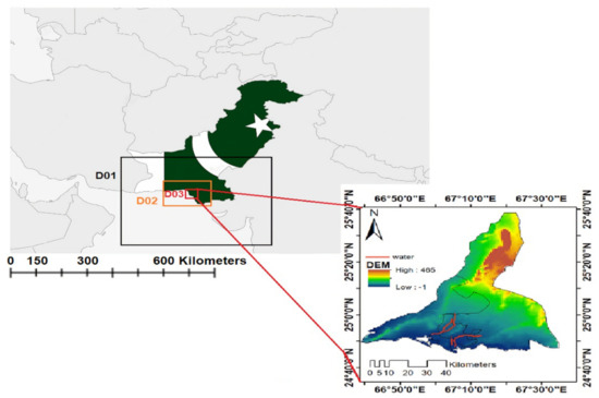
Figure 2.
Study area and WRF model domain location. (D03 is covering study area).
2.2. Model Configuration and Data
In present study, the WRF model version 4.0 was used which is a mesoscale model [17] and widely applied in the teaching community as well as science. The WRF model is ideal for spatial scales ranging from meters to hundreds of kilometers [54]. The model was run to simulate heat waves in Karachi, from 16–23 May 2018. During the WRF run a spin-up phase of model was considered on 16 May 0000 UTC and withdrawn from the study 24 h later.
The initial boundary conditions were derived from the NCEP FNL global operational analysis and forecasted every six hours on a 0.25° × 0.25° grids https://rda.ucar.edu (accessed on 9 September 2019). The WRF model configuration involves a two-way nesting and a 1:3 nesting grid ratio, with a horizontal scale ranging from 9 km × 9 km for the coarse domain (d01, 200 × 184 grid cells; Figure 1) to 3 km × 3 km for the middle domain (d02, 129 × 129 grid cells) to 1 km × 1 km for the innermost domain containing the study area (d03, 120 × 114 grid cells). The model outputs were obtained in an hourly interval. T(max-WRF) was validated with ground station data from the Pakistan meteorological department and simulated heat fluxes (LH&SH) were evaluated against the Climate Forecast system reanalysis data (CFSR) https://app.climateengine.org/climateEngine (accessed on 28 August 2021) using the error finding models as explained in Section 3.3. ENSO is the most crucial atmosphere driver of climate system, we extended this analysis, to study the relationship between ENSO and heat wave event in Karachi node, Pakistan https://sealevel.jpl.nasa.gov/ (accessed on 28 August 2021).
2.3. Experimental Design
WRF version 4.0 has different land surface physics options. The WRF land surface models are driven by water and energy fluxes and moisture in soil layers and predicted soil temperature depending on the LSS option in which RUC has 9 layers, and NOAH and NOAH_MP has four layers. All the WRF LSS utilize the information from the atmospheric surface layer scheme such as wind. In WRF, all the model atmospheric setting were exactly the same except for the LSS. The Rapid Radiative Transfer Model (RRTM) is used for describing long wave radiation transfer to surface and within the atmosphere, and the shortwave scheme selected was developed by Dudhia [55,56]. The microphysics scheme chosen is the WRF Single–Moment 3-class (WSM3) scheme [57]. The Kain-Fritch convection scheme is selected to parameterize cumulus clouds [58]. The Yonsei University (YSU) planetary boundary layer (PBL) scheme is applied to deal with boundary layer processes [59]. It was designed with a different set of schemes to see how different physics schemes affected the simulation of a heat wave in Karachi, Pakistan. Figure 3 and Table 1 have a description of the entire setups. The setups namely are E1, E2, and E3. The cumulus parameterization scheme was not used in d03, because the simulation of the high resolution (1 km × 1 km) was adopted here. This selection was made on the preliminary tests that agreed with the findings of Gbode, I.E., et al. (2019) [60].
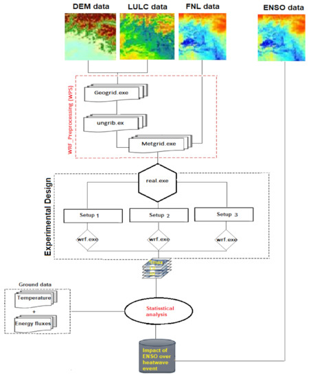
Figure 3.
Brief methodology flow chart with WRF model preprocessing steps.

Table 1.
Details of different setups under schemes used in the WRF model.
The NOAH LSS was validated by many studies both in coupled [61,65] and uncoupled mode [66,67]. National Center for Atmospheric Research (NCAR) and National Centers for Environmental Prediction (NCEP) jointly developed NOAH model [68]. It works well in operational weather and climate models because of its moderate complexity and computational efficiency. It is compatible with NCEP’s global analysis datasets that include soil fields. In Table 2 it can be seen that it includes a soil temperature and moisture model with four layers (0.10, 0.30, 0.60, and 1 m deep), as well as canopy moisture and snow cover prediction. A surface energy balance equation is used to compute the skin surface temperature. Noah’s surface energy fluxes are estimated over a mixed vegetation and bare soil layer. Since it cannot explicitly compute photosynthetically active radiation (PAR), canopy temperature, and related energy, water, and carbon fluxes, such a model restricts its further development as a process based dynamic leaf model [62].
Table 2.
Main characteristics of LSS (NOAH, NOAH_MP, RUC).
NOAH-MP (multiphysics) LSS is a sequel to the Noah model. The most important enhancement is the addition of (1) a vegetation canopy layer for computing individual canopy and ground surface temperatures that is accomplished by using semitile subgrid approach to reflect land surface heterogeneity [69], (2) a modified two stream scheme for radiation transfer through vegetation canopy while accounting for canopy gaps, (3) a Ball Berry scheme for canopy stomatal resistance that links stomatal resistance to photosynthesis of sunlit and shaded leaves, and (4) a short term dynamic vegetation model with two options (on/off) in which leaf area index (LAI) and vegetation greenness fraction (GVF) may be predicted from the model as turned on. For major land-atmosphere interaction processes, the NOAH-MP employs a variety of choices. It has a distinct plant canopy characterized by a canopy top and bottom, as well as leaf physical and radiometric attributes which are used in a two-stream canopy radiation transmission method with shading effects. NOAH-MP includes multilayer snowpack with liquid water storage and refreeze/melt capacity, as well as a snow-interaction model that describes canopy intercepted snow melt/refreeze, loading/unloading, and simulation shown in Table 2. A variety of alternatives are available for surface water penetration and runoff, as well as groundwater transfer and storage, including water table depth.
RUC LSS is primarily concerned with accurate soil characterization up to 6–9 soil levels, down to a depth of 300 cm [70] as presented in Table 2. RUC has a good understanding of snow physics and soil phase shift. It solves the heat diffusion and Richard’s moisture transfer equations at six or more levels [70,71]. Clapp and Hornberger (1978) show soil moisture coefficients as functions of 11 textural classifications of soil plus peat. STATSGO, a 16-category soil categorization system, is utilized in RUC [72]. With appropriate heat capacities and densities, energy, and moisture budgets are solved in a thin layer spanning the ground surface and encompassing half of the topsoil layer and half of the first atmospheric layer, having heat capabilities and densities that match. The impact vegetation on evaporation is considered, with canopy moisture serving as a predictive variable and evapotranspiration parameters varying by vegetation type [73,74].
2.4. Model Evaluation
A wide range of statistical methods are available to judge a model’s performance and credibility [75]. The difference between simulated and observed values was calculated using the error statistics in this study, and the performance of the WRF model was gauged. We used the average grid value simulated with WRF and the station data point value. Statistical error indicators, such as BAISE, mean absolute error (MAE), root means square error (RMSE), coefficient correlation (R), agreement index (IOA), and Nash-Sutcliffe efficiency (NES), were used to evaluate model performance in simulation of maximum temperatures during the heat wave event. The equations and formulas are following [34].
where is the value of observed parameter and is the simulated values of parameter obtained from the WRF model. Furthermore, the efficiency of the predictive power of WRF model was assessed using the NSE coefficient in different physical schemes. The NSE coefficient indicates how best the simulation model is; ranges of 0–0.3, 0.3–0.6, 0.6–0.8, and above 0.8 imply poor, reasonable, good, and excellent, predictive capacity, respectively [76,77].
3. Results
In this section, the simulated WRF results of daily maximum temperature at 2 m T(max_WRF), latent heat LH(WRF), and sensible heat SH(WRF) from 16–23 May 2018 were evaluated by comparing with ground observations to investigate the performances of different WRF schemes.
3.1. Daily Temperature Maximum Analysis
T(max_WRF) was plotted against the in-situ measurements T(max_OBS) in Figure 4, and it was discovered that all setups have a different correlation with the T(max_OBS).
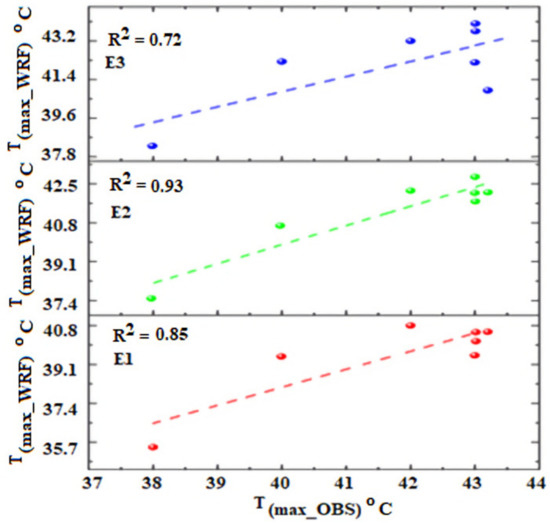
Figure 4.
Scatter plot between T(max_OBS) and WRF simulated T(max_WRF) with different setups.
E2 simulated T(max) very similar to T(max_OBS) while E1 and E3 underestimated and overestimated T(max) shown in Figure 5a, respectively. Figure 5b shows the difference of T(max) and T(mean) during the heatwave period. All setups showed the positive difference that means extreme temperature condition (heatwave). The E2 is an ideal setup, it showed low difference (8.2 °C) on 20 May 2018 and high difference (9.2 °C) on 21 May 2015. Overall, the E2 and E3 setups overestimated the T(max) as compared to T(max_OBS), but the E1 scheme showed underestimating the T(max) during the whole period of heat wave. Figure 6 on 18 May, the temperature became lower as compared to other days with the heat-wave event.
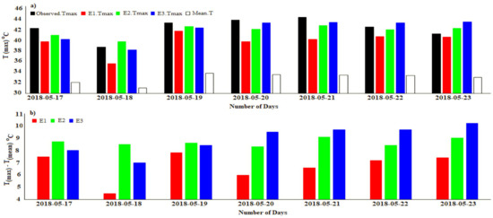
Figure 5.
(a) Daily temporal variation of T(max_WRF) and T(max_OBS), (b) difference between T(max) and T(mean) during the heat-wave period.
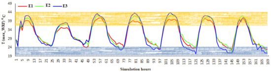
Figure 6.
Hourly variation of T(max_WRF) using three different setups for the period of 7 days. Orange = high T(max_WRF) and Blue = low T(max_WRF).
The spatial distribution of T(max) was exhibited during the daytime (11:00) and nighttime (21:00) UTC is represented in Figure 7 and showed the high temperature during day and low temperature at night in Karachi. The east-south region is warmer and experienced high temperatures magnitude during day. During the nighttime, E1 and E2 showed temperature of urban area is higher while E3 simulated the lower temperature of urban region. In comparison to the urban and east-south parts of Karachi, the west-south area of the city has a lower temperature. Table 3 mainly describes the comparisons between T(max_WRF) and T(max_OBS) based on different WRF setups for the heat-wave duration. Statistical error identifying parameters: BIAS, MAE, R, RMSE, NSE, and IOA were computed to determine the efficiency of temperature simulation (E1, E2, and E3) are listed in Table 3. It is noted that the R2 of T(max_WRF) in E2 (0.93) based on model simulation is higher than the E1 (0.85), and E3 (0.72) based on the model simulation during the heat wave event.
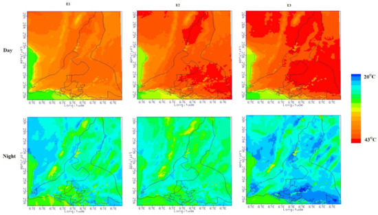
Figure 7.
Spatial distribution of hourly T(max_WRF) (°C) at UTC 11:00 (Daily) and 21:00 (Night) on 20 May 2018. (E1 = first setup; E2 = second setup; and E3 = third setup).
Table 3.
Statistics of T(max-WRF), LHWRF, and SHWRF during the heat wave (16–23 May 2018) with different LSS in the WRF4.0 model. BIAS, daily mean difference; MAE, the daily mean of absolute error; RMSE, the daily mean of root means squared error; R, mean of spatial correlation coefficient and IOA, mean of the index of agreement.
The E2 shows higher R2 and lower RMSE, BIASE, MAE compared to E1 and E3. The RMSEs for E1, E2, and E3 against observation are 3.38 °C, 1.13 °C, and higher 2.65 °C respectively. At the same time, the MAEs of T(max_WRF) for E1 (2.27 °C), and E3 (1.25 °C) is higher than that of E2 (0.69 °C). The BIAS value for the E2 is 0.69 °C and the higher value is 2.27 °C for the E1 as displayed in Figure 8. Overall, it is noted that the IOA of temperature simulation in E2 (0.94) is higher than the E2 (0.72), and E3 (0.84) based on model simulation. Besides, the reliability of WRFV4.0′s predictive capacity using various setups was measured using the NSE coefficient. In the present analysis, the NSE coefficient values are 0.73, 0.84, and 0.77 for E1, E2, and E3, respectively. Throughout the entire heat wave period, E2 has the lowest RMSE, BIAS, and MAE. On the other hand, E3 well-simulated T(max_WRF) on May 18 and 20, 2018 with the lowest BIAS and MAE errors relative to other days and E1 simulated T(max_WRF) with a higher BIAS and MAE errors. Overall results depicted that T(max_WRF) from E2 setup is quite better in Karachi, Pakistan as compared to E1 and E3 as shown in Table 3.
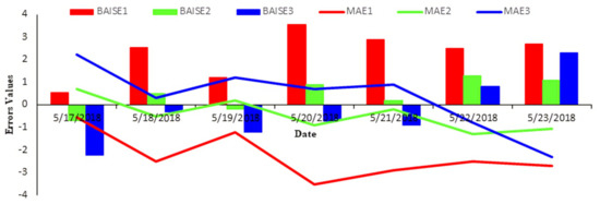
Figure 8.
Daily T(max_WRF) mean BIAS and MAE during the heat wave period by using three different setups.
During the May 2018 heat wave, E3 overestimated the T(max_WRF) while E1 underestimated. The overall BIAS, MAE, RMSE, and IOA values for E3 were found as −0.32 °C, 1.2 °C, 2.65 °C, and 0.84 °C, respectively. E1 underestimated the T(max_WRF) and it has significant BIAS and MAE values suggested that the T(max) during the entire heat wave period was not simulated well. E3 was known as the second best WRF setup to measure T(max) according to the error matrix since it has the lowest errors (BIAS, MAE, RMSE) compared to E1.
3.2. Surface Energy Fluxes Analysis
Surface heat energy fluxes (LH and SH) are very important for understanding the meteorology that is simulated near-surface. The description of three setups E1, E2, and E3 are showed in Table 1. Simulated LH&SH were evaluated against the Climate Forecast System Reanalysis (CFSR) data and freely accessible at https://app.climateengine.org/climateEngine (accessed on 12 June 2020). The LHWRF and SHWRF were modeled using three different setups (E1, E2, and E3) during the heat wave event. To determine the discrepancies between the WRF simulated and satellite-based fluxes different statistical error measuring parameters were used namely BIAS, MAE, RMSE, R, and IOA. Statistical error matrix: BIAS, MAE, R, RMSE, NSE, and IOA were determined to study the efficiency of simulation of model for LH based on E1, E2, and E3 as showed in Table 3. The E2 shows higher R2 and lower RMSE, BIASE, MAE compared to E1 and E3. It can be seen from Figure 9 that R2 of LHWRF (SHWRF) in E2 0.99(0.99) based on model simulation is higher than the E1 0.98(0.98), and E3 0.96(0.99) based on the model simulation during the heat wave event. The RMSEs for E1, E2, and E3 against observation are 62.30 wm−2 (21.71 wm−2), 44.60 wm−2 (26.24 wm−2) and higher 61.50 wm−2 (50.94 wm−2), respectively. At the same time, the MAEs of LHWRF (SHWRF) for E1 61.08 wm−2 (51.11 wm−2), and E3 65.34 wm−2 (24.87 wm−2) is higher than that of E2 42.27 wm−2 (50.26 wm−2). Besides, IOA was computed to know the exact accuracy of simulated results that were 0.99 and 0.99 for LH and SH simulation using the E2 setup. It can be concluded that E2 is best to reproduce LH and SH fluxes because it has low errors (RMSE, MAE, and BAIS) and the highest IOA while the other two setups E1 and E3 are showing high errors and lowest IOA. The NSE coefficient depicts that E2 performed better to simulate the energy fluxes including LH and SH with value 0.89.
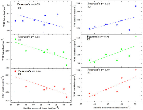
Figure 9.
Scatter plot between mean daily satellite measured latent heat, sensible heat and WRF simulated latent heat, sensible heat during the heat wave period.
During the daytime, the modeled profile of surface energy fluxes for all setups is shown a positive trend while a negative trend at nighttime. The patterned profiles based on three setups gave different results. E2 has been declared the most appropriate setup in Section 3.1. SH is a means of moving energy from one system to another without altering the physical state of the system; SH value is positive during the day, indicating that energy is released from the surface to the atmosphere and reaches its peak value during the daytime as shown in Figure 10. The SH profile at night is negative which means energy is transferred from the ambient surrounding to the ground surface. During day and night, E1, E2, and E3 simulated similar SH patterns. It can be observed that on 18 May 2018 nighttime (17:00–22:00) all setups were measuring maximum negative flux value. The maximum peak value calculated by the E1 is 412 wm−2 at 8:00 and the minimum peak value is −37 wm−2 on 18 May 2018. E2 assessed SH with a maximum peak value of 486 wm−2 at 07:00 and a minimum peak value of −48 wm−2 at 18:00 on 18 May 2018.
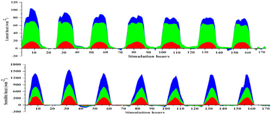
Figure 10.
Time series of LHWRF (Wm−2) and SHWRF (Wm−2) using three setups during the heat wave period Karachi.
E3 calculated SH flux value and simulated a maximum peak value of 646 wm−2 on 18 May 2018 during the day at 07:00 and a minimum peak value of −50 wm−2 at 24:00 on 18 May 2018. SH profile showed that on 21 May 2018 there is a sharp decrease from 353 wm−2 to 331 wm−2 in SH signature based on E2 while also the same sharp decrease was observed on 23 May 2018 for E3 at 06:00 with a change from 400 wm−2 to 276 wm−2. No sharp change has been observed for E1 during the heat-wave period. LH was lower than SH during the entire heat wave event. E2 simulated that LH reached a maximum value of 59 wm−2 at 04:00 and on 2018 May 18 unexpectedly dropped to 49 wm2 at 05:00. LH contributed maximum during the 02:00–12:00 as shown in Figure 10.
Figure 10 and Figure 11 showed that the spatial pattern of LH and SH is lower at night and higher during the day. Figure 11 shows a lower value in the urban area during the day and the same value at night. The WRFLH is showing a higher magnitude throughout the day and night along the coastal line. SHWRF shows the opposite pattern to LHWRF. Conversely, SHWRF is higher in the urban area, especially during the day, and lower at night, as seen in Figure 12. SHWRF is showing a low magnitude in day and night along the coastal line.
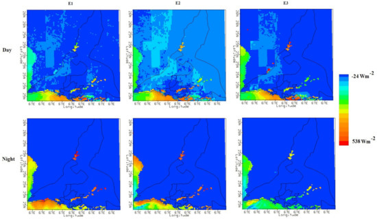
Figure 11.
Spatial distributions of hourly LHWRF (Wm−2) using different setups (E1, E2, and E3) at 10:00 (day) and 21:00 (Night) UTC on 2018 May 20 during heat wave period Karachi (E1 = first setup; E2 = setup; and E3 = third setup).
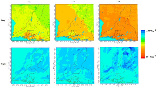
Figure 12.
Spatial distributions of hourly SHWRF (Wm−2) using different setups (E1, E2, and E3) at 10:00 (day) and 21:00 (Night) UTC on 20 May 2018 during heat wave period Karachi. (E1 = first setup; E2 = second setup; and E3 = third setup).
3.3. The Role of Ocean-Atmospheric Coupling
The super EL Nino of 2015–16 was the most powerful in the 21st century thus far. There are similarities between El Nino events, each one has a particular timing and different in impacts. The El Nino event of 2015–16 lasted longer and covered a larger area than the one of 1997–98. Figure 13 shows the anomalies in Pacific Ocean sea surface height (SSH) anomalies during May 2015–16 event. De-trended Temperature anomaly based on monthly means of 2015 was regressed onto the standardized Nino-3.4 index. The correlation was calculated between Nino-3.4 and the temperature anomalies. It shows that the climate variability is linked to ENSO. Figure 14 shows the effects of ENSO over the globe, as well as the association between warm states El Nino with temperature anomalies.
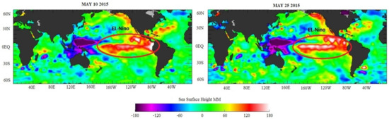
Figure 13.
Central Pacific El Niño event information May 2015.
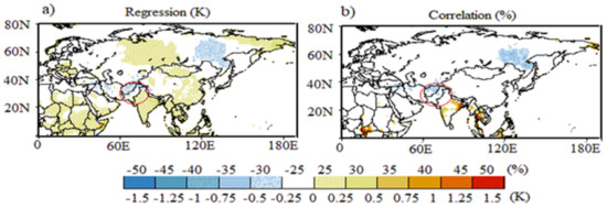
Figure 14.
Correlation between DE trended temperature and standardized Niño-3.4 index during MJJ 2015.
The difference in sea surface temperature between the Arabian Sea and eastern Indian Ocean forms the IOD. The During the study period May 2015, El Nino events were occurred causing positive IOD events [78].
The atmospheric circulation pattern over Arabian Sea was investigated and analyzed to better understand the causes of heat wave occurrence in Karachi node, as illustrated in Figure 15. El Nino 3.4 events resulted in a positive IOD in the western Indian Ocean, reducing cloudiness and moisture levels over adjoining areas of Indian Ocean basin [79,80,81]. The persistence and strengthening of heat wave over Karachi node were largely due to atmospheric circulation patterns. Normal moisture was transported from the Arabian Sea during the month of May (15–16), shown in Figure 15. A ridge was formed over the coastal areas, including Karachi, on 17 May 2015, and atmospheric circulation went anomalous. The sea winds were blocked due to high pressure over the Karachi and low pressure over Arabian Sea. Consequently, it reduced the humidity level and stopped the moisture transportation. The ridge was maintained till 23 May 2015, prolonging the heat wave in the area. Meanwhile, during the heat wave period wind patterns over Karachi remained easterly due to low pressure zones in the northeast Arabian Sea and Bay of Bengal as in Figure 16.
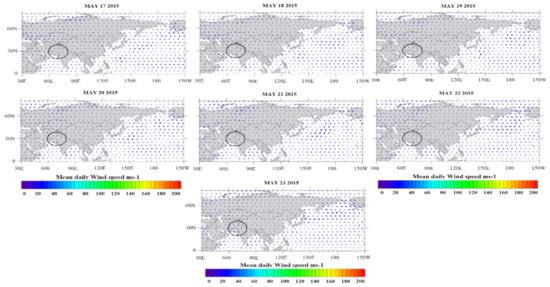
Figure 15.
Mean daily wind speed variation during the heat wave event at Karachi.
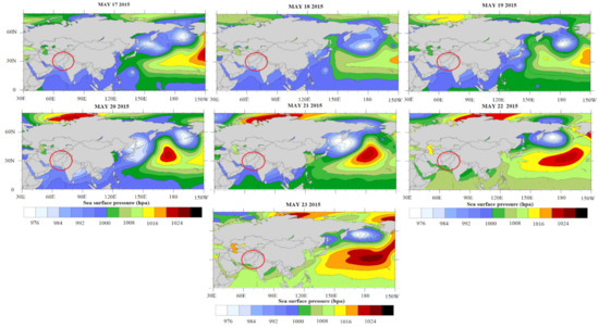
Figure 16.
Mean daily surface pressure variation during the heat wave event at Karachi.
4. Discussion
Rapidly changing weather patterns, including mean warming, rising mean minimum temperature, and rainfall patterns, are causing an increase in the frequency and intensity of heat waves. A best combination of LSS in WRF model in a certain study area may increase the heat wave response and preparedness ability. Pakistan is going through a period of intensive dynamic climate change that may bring unwanted variations in temperature, rainfall, and wind patterns. The heat wave is a climatic hazard, leading to severe damage to life, particularly in vulnerable communities. It is critical to employ NWP skills and RCMs like as WRF to study extreme events in the present and future. Different parameterizations are added into RCMs to simulate extreme weather events that have typical systematic biases yet even after a long history of major development in terms of spatial resolution as well as introducing various physical processes. Later, the RCM was combined with urban canopy models as well as LSMs to apprehend different urban structure to simulate accurately heat wave-related mechanisms.
It can be helpful to be responsive and adaptive to hazards in the future. In the present research, we used WRF model to evaluate the sensitivity of combination of physics schemes and it integrates several choices for parameterizing microphysics of the surface layer, cumulus parameterization, PBL, ground surface, and clouds. Researchers previously used the WRF model to simulate meteorology, but due to change in simulation time, study region, weather conditions, and important goals, their WRF setting combination is not generally applicable. The key goal of the current research is to find the best surface scheme in the WRF model (4.0) to simulate the heat wave event over Karachi, Pakistan. We used three LSS (Noah, Noah-MP, and RUC) in the mesoscale model WRF, Version4.0, to study the sensitivities of T(max) and energy fluxes to different LSS. We designed three setups (E1, E2, and E3) to simulate heat wave event on 16–23 May 2018 in Karachi, node. The present study resulted that Noah-MP produced better daily mean T(max) as compared to Noah and RUC LSS. Overall, Noah underestimated, and RUC LSS overestimated daily mean T(max) during the heat wave event. In the case of energy fluxes (LH&SH), it was determined that Noah-MP is best LSMs for simulating LH and SH fluxes since it has the low errors and highest IOA whereas the other LSS (Noah, and RUC) are showing high errors and lowest IOA. Similarly, Reddy, Srinivas et al. (2020) investigated the impact of land surface physics in WRF on the simulation of sea breeze circulation over the southeast coast of India and resulted that the Noah-MP (LSS) produced a more realistic simulation of air temperature and heat fluxes [82]. Constantinidou, Hadjinicolaou et al. (2020) concluded during the study the performance of LSMs in the WRF model for climate simulation over the MENA-CORDEX domain that Noah-MP simulations are closest to observations [83]. Noah-MP performed well because it incorporates 1-layer canopy, 3-layer snow, and 4-layer soil as well as an interactive energy balance to simulate surface temperature, and a modified two-stream radiation transfer scheme to consider the 3D-canopy.
In our study, temperature is higher in daytime while lower in night. Urbanization caused changes of aerodynamics resistance, ground heat fluxes, and long wave emissivity. It decreases wind speed that would increase the aerodynamics resistance, which is in favor of a weak SH and low temperature in night. The SH flux played a larger role in stimulating the heat wave event in May 2018 due to dense urban canopy, and less vegetated region. It contributes higher than LH to intensify heat waves. The absorbed energy was used to create water vapors from soil moisture, vegetation, and evaporation. This accumulated energy is released into the atmosphere during cloud formation and becomes heated. In the presence of electromagnetic radiations, the Planet is constantly receiving energy from the sun and getting colder. Even at night, the Earth stores energy and transmits the transmission phenomenon: LH, SH is continued until it becomes normal. This energy transfer contributes to the rise in ambient temperature. The difference in temperature between surface and atmosphere makes it possible to induce more processes that may be a cause for temperature rises. Energy is transmitted to the atmosphere during the positive SH cycle, resulting in a decrease in surface pressure as air molecules are transported upward.
El Nino reduces cloudiness, resulting in drier conditions in the affected regions. Day time temperatures are warmer than normal during the El Nino events, and increased evaporation is worsening the effect of lower-than-normal rainfall. The difference in sea surface temperature between the Arabian Sea and eastern Indian Ocean forms the IOD. The IOD phenomena effects the climate of countries along the Indian Ocean Basin including Australia and is a major contributor to temperature and rainfall variability in the region [84,85,86,87]. Through an expansion of Walker Circulation to west and linked Indonesian through flow, IOD has been associated with ENSO episodes. El Nino 3.4 events resulted in a positive IOD in the western Indian Ocean, reducing cloudiness and moisture levels over adjoining areas of Indian Ocean basin. The sea winds were blocked due to high pressure over the Karachi and low pressure over Arabian Sea. The ridge was maintained till 23 May 2015, prolonging the heat wave in the area.
It is very important to know the uncertainties occur in the current study. First, the findings of the present study were derived through numerical simulations, therefore the parametric and structural uncertainties of the WRF model need to be further constrained. Second, to count the problem of systematic errors and to minimize the model drift from the initial boundary conditions, the WRF simulation in this study should have reinitialized every day. This technique would improve the performance of the WRF model prediction at fine scale. The intensity of heat wave changes with local climate. It would be recommended to study the feature of heat waves in different climate zones. In context to climate change mitigation and strategy point of view, the results of this study have significant implications regarding the simulation and projection of regional climate. To combat the harmful effects of heat waves and their synergistic interactions in the climate change condition, particularly urban adaptation strategies are required.
5. Conclusions
This study used the WRF model coupled with three different LSS (NOAH, NOAH_MP, and RUC) and quantitatively evaluated the role of land surface processes in the regional climate (heat wave). The coupling of different LSS represent our most recent effort to improve the land surface simulation in the regional climate. Results show that the selection strongly of LSS affect the temperature simulations. The performance of the WRF model in simulating the temperature and energy fluxes (LH&SH) and their relation with the pacific variability were first evaluated and then concluded flowing points:
- Overall based on statistical analysis, E2 performs best to simulate T(max), LH, and SH during the heat wave events. It is concluded that E2 works best for the present study area and may be used to simulate the other meteorological variables for further implementation of the WRF model. Noah_MP (LSS) performs better than the Noah and RUC.
- Results concluded that surface physics schemes like the Noah MP function well with the higher NSE, agreement, and low errors compared to the RUC, and Noah (LSS) to predict the T(max) and LH&SH. The combination of Dudhia short wave, RRTM long wave, and Noah_MP parameterization schemes best to simulate the heat wave events.
- The combination of Dudhia short wave, RRTM long wave, and RUC LSS overestimated T(max), LH, and SH fluxes with larger BIAS, MAE, RMSE, and low IOA respectively when compared with ground observations.
- Noah-MP model gives better results because it considers the multi-surface temperatures and distinct canopy to forecast while the other model does not account for such multi-surface temperatures. Noah-MP forecasts the temperature same to reality based on considering the multi factors: temperature leaf, temperature canopy, temperature snow, and temperature ground.
- ENSO event 2015–16 and atmospheric circulation played vital role to prolong and strengthen the heat wave in Karachi, Pakistan. EL Nino event modifies the IOD that stopped the moisture transportation along the coastal regions.
More through modelling experiments are necessary to better estimate the temperature in WRF, more extensive modelling experiments are required. These setups comprise tests with several combinations of different cumulus schemes, micro physics schemes, radiation schemes, and PBL schemes that have been coupled in the state-of-the-art WRF model.
Author Contributions
Conceptualization, B.C. and A.D.; methodology, A.D., B.C. and S.L.; software, A.D.; validation, A.D., A.A. and Y.H.; formal analysis, A.D., investigation, A.D., S.L., A.A., M.A.Q., A.K., Y.H., H.Z. and F.W.; resources, B.C.; data curation, A.D., A.A., S.M., Y.H., L.G., M.S.; writing—original draft preparation, A.D.; writing—review and editing, B.C., A.D. and A.A.; visualization, A.D.; supervision, B.C.; project administration, B.C.; funding acquisition, B.C. All authors have read and agreed to the published version of the manuscript.
Funding
This work was supported by the Strategic Priority Research Program of Chinese Academy of Sciences (Grant No. XDA 20030302), the National Key R&D Program of China [Grant # 2018YFA0606001 & 2017YFA0604301], the research grants [41771114 & 41271116] funded by the National Natural Science Foundation of China, and the research grant [O88RA901YA] funded by the State Key Laboratory of Resources and Environment Information System.
Institutional Review Board Statement
Not applicable.
Informed Consent Statement
Not applicable.
Data Availability Statement
Data sharing is not applicable to this article as no new data was generated.
Acknowledgments
First author wants to thank National Center for Atmospheric Research (NCAR), https://ncar.ucar.edu/ (accessed on 12 January 2019) and Computational and the Research Data Archive managed by Information System Laboratory https://rda.ucar.edu/ (accessed on 9 September 2019) for proving open access WRF model and its inputs data. Also, thanking to Jet Propulsion Laboratory, California Institute of Technology under The National Aeronautics and Space Administration (NASA) https://sealevel.jpl.nasa.gov/ (accessed on 28 August 2021) for providing open access data for ENSO.
Conflicts of Interest
The authors declare no conflict of interest.
References
- IPCC. Intergovernmental Panel on Climate Change. 2013. Summary for Policymakers of Climate Change 2013: The Physical Science Basis. Contribution of Working Group I to the Fifth Assessment Report of the Intergovernmental Panel on Climate Change; Cambridge University Press: Cambridge, UK, 2013. [Google Scholar]
- Ciais, P.; Reichstein, M.; Viovy, N.; Granier, A.; Ogée, J.; Allard, V.; Aubinet, M.; Buchmann, N.; Bernhofer, C.; Carrara, A.; et al. An unprecedented reduction in the primary productivity of Europe during 2003 caused by heat and drought. Nature 2005, 437, 529–533. [Google Scholar] [CrossRef] [PubMed]
- Dai, A. Increasing drought under global warming in observations and models. Nat. Clim. Chang. 2012, 3, 52–58. [Google Scholar] [CrossRef]
- Shrestha, N.K.; Wang, J. Water Quality Management of a Cold Climate Region Watershed in Changing Climate. J. Environ. Inform. 2019, 35. [Google Scholar] [CrossRef]
- Sun, W.; Mu, X.; Song, X.; Wu, D.; Cheng, A.; Qiu, B. Changes in extreme temperature and precipitation events in the Loess Plateau (China) during 1960–2013 under global warming. Atmos. Res. 2016, 168, 33–48. [Google Scholar] [CrossRef]
- Hanif, U. Socio-Economic Impacts of Heat Wave in Sindh. Pak. J. Meteorol. 2017, 13, 87–96. [Google Scholar]
- Perkins, S.E.; Alexander, L.; Nairn, J.R. Increasing frequency, intensity and duration of observed global heatwaves and warm spells. Geophys. Res. Lett. 2012, 39, 1053361. [Google Scholar] [CrossRef]
- Saeed, F.; Salik, K.M.; Ishfaq, S. Climate Induced Rural-to-Urban Migration in Pakistan. 2016. Available online: https://sdpi.org/ (accessed on 19 January 2016).
- Zahid, M.; Rasul, G. Rise in summer heat index over Pakistan. Pak. J. Meteorol. 2010, 6, 85–96. [Google Scholar]
- Beniston, M.; Stephenson, D.B.; Christensen, O.B.; Ferro, C.A.T.; Frei, C.; Goyette, S.; Halsnæs, K.; Holt, T.; Jylhä, K.; Koffi, B.; et al. Future extreme events in European climate: An exploration of regional climate model projections. Clim. Chang. 2007, 81 (Suppl. 1), 71–95. [Google Scholar] [CrossRef] [Green Version]
- Giorgi, F.; Bates, G.T. The climatological skill of a regional model over complex terrain. Mon. Weather. Rev. 1989, 117, 2325–2347. [Google Scholar] [CrossRef] [Green Version]
- Li, Z.; Li, J.J.; Shi, X.P. A Two-Stage Multisite and Multivariate Weather Generator. J. Environ. Inform. 2019, 35, 424. [Google Scholar] [CrossRef]
- Feudale, L.; Shukla, J. Influence of sea surface temperature on the European heat wave of 2003 summer. Part I: An observational study. Clim. Dyn. 2010, 36, 1691–1703. [Google Scholar] [CrossRef]
- Kharin, V.V.; Zwiers, F.W.; Zhang, X.; Hegerl, G. Changes in Temperature and Precipitation Extremes in the IPCC Ensemble of Global Coupled Model Simulations. J. Clim. 2007, 20, 1419–1444. [Google Scholar] [CrossRef] [Green Version]
- Fischer, E.M.; Seneviratne, S.; Lüthi, D.; Schär, C. Contribution of land-atmosphere coupling to recent European summer heat waves. Geophys. Res. Lett. 2007, 34, 1029068. [Google Scholar] [CrossRef] [Green Version]
- Ren, J.; Huang, G.; Li, Y.; Zhou, X.; Lu, C.; Duan, R. Stepwise-clustered heatwave downscaling and projection for Guangdong Province. Int. J. Clim. 2021. [Google Scholar] [CrossRef]
- Skamarock, W.C.; Klemp, J.B.; Dudhia, J.; Gill, D.O.; Barker, D.M.; Wang, W.; Powers, J.G. A Description of the Advanced Research WRF; Version 3; National Center for Atmospheric Research: Boulder, CO, USA, 2008. [Google Scholar]
- Shrivastava, R.; Dash, S.K.; Oza, R.B.; Sharma, D.N. Evaluation of Parameterization Schemes in the WRF Model for Estimation of Mixing Height. Int. J. Atmos. Sci. 2014, 2014, 451578. [Google Scholar] [CrossRef] [Green Version]
- Sellers, P.J.; Dickinson, R.E.; Randall, D.A.; Betts, A.K.; Hall, F.G.; Berry, J.A.; Collatz, G.J.; Denning, A.S.; Mooney, H.A.; Nobre, C.A.; et al. Modeling the exchanges of energy, water, and carbon between continents and the atmosphere. Science 1997, 275, 502–509. [Google Scholar] [CrossRef] [Green Version]
- Jin, J.; Miller, N.L.; Schlegel, N.-J. Sensitivity Study of Four Land Surface Schemes in the WRF Model. Adv. Meteorol. 2010, 2010, 167436. [Google Scholar] [CrossRef] [Green Version]
- Lhotka, O.; Kyselý, J.; Plavcová, E. Evaluation of major heat waves’ mechanisms in EURO-CORDEX RCMs over Central Europe. Clim. Dyn. 2018, 50, 4249–4262. [Google Scholar] [CrossRef]
- Zeng, X.-M.; Wu, Z.; Xiong, S.; Song, S.; Zheng, Y.; Liu, H. Sensitivity of simulated short-range high-temperature weather to land surface schemes by WRF. Sci. China Earth Sci. 2011, 54, 581–590. [Google Scholar] [CrossRef]
- Zittis, G.; Hadjinicolaou, P. The effect of radiation parameterization schemes on surface temperature in regional climate simulations over the MENA-CORDEX domain. Int. J. Clim. 2016, 37, 3847–3862. [Google Scholar] [CrossRef]
- Zittis, G.; Hadjinicolaou, P.; Lelieveld, J. Comparison of WRF Model Physics Parameterizations over the MENA-CORDEX Domain. Am. J. Clim. Chang. 2014, 3, 490–511. [Google Scholar] [CrossRef] [Green Version]
- Bucchignani, E.; Cattaneo, L.; Panitz, H.-J.; Mercogliano, P. Sensitivity analysis with the regional climate model COSMO-CLM over the CORDEX-MENA domain. Theor. Appl. Clim. 2016, 128, 73–95. [Google Scholar] [CrossRef]
- Constantinidou, K.; Hadjinicolaou, P.; Zittis, G.; Lelieveld, J. Sensitivity of simulated climate over the MENA region related to different land surface schemes in the WRF model. Theor. Appl. Clim. 2020, 141, 1431–1449. [Google Scholar] [CrossRef]
- Davin, E.L.; Maisonnave, E.; Seneviratne, S.I. Is land surface processes representation a possible weak link in current Regional Climate Models? Environ. Res. Lett. 2016, 11, 074027. [Google Scholar] [CrossRef]
- Soares, P.M.M.; Careto, J.A.M.; Cardoso, R.M.; Goergen, K.; Trigo, R.M. Land-Atmosphere Coupling Regimes in a Future Climate in Africa: From Model Evaluation to Projections Based on CORDEX-Africa. J. Geophys. Res. Atmos. 2019, 124, 11118–11142. [Google Scholar] [CrossRef]
- Knist, S.; Goergen, K.; Buonomo, E.; Christensen, O.B.; Colette, A.; Cardoso, R.M.; Fealy, R.; Fernández, J.; García-Díez, M.; Jacob, D.; et al. Land-atmosphere coupling in EURO-CORDEX evaluation experiments. J. Geophys. Res. Atmos. 2017, 122, 79–103. [Google Scholar] [CrossRef] [Green Version]
- Sun, Y.; Hu, T.; Zhang, X. Substantial Increase in Heat Wave Risks in China in a Future Warmer World. Earth’s Futur. 2018, 6, 1528–1538. [Google Scholar] [CrossRef] [Green Version]
- Mortezazadeh, M.; Jandaghian, Z.; Wang, L.L. Integrating CityFFD and WRF for modeling urban microclimate under heatwaves. Sustain. Cities Soc. 2021, 66, 102670. [Google Scholar] [CrossRef]
- Patil, R.; Kumar, P.P. WRF model sensitivity for simulating intense western disturbances over North West India. Model. Earth Syst. Environ. 2016, 2, 82. [Google Scholar] [CrossRef] [Green Version]
- Tian, Y.; Miao, J. A Numerical Study of Mountain-Plain Breeze Circulation in Eastern Chengdu, China. Sustainability 2019, 11, 2821. [Google Scholar] [CrossRef] [Green Version]
- Gunwani, P.; Mohan, M. Sensitivity of WRF model estimates to various PBL parameterizations in different climatic zones over India. Atmos. Res. 2017, 194, 43–65. [Google Scholar] [CrossRef]
- Mohan, M.; Gupta, M. Sensitivity of PBL parameterizations on PM10 and ozone simulation using chemical transport model WRF-Chem over a sub-tropical urban airshed in India. Atmos. Environ. 2018, 185, 53–63. [Google Scholar] [CrossRef]
- Sathyanadh, A.; Prabha, T.V.; Balaji, B.; Resmi, E.; Karipot, A. Evaluation of WRF PBL parameterization schemes against direct observations during a dry event over the Ganges valley. Atmos. Res. 2017, 193, 125–141. [Google Scholar] [CrossRef]
- Zeyaeyan, S.; Fattahi, E.; Ranjbar, A.; Azadi, M.; Vazifedoust, M. Evaluating the Effect of Physics Schemes in WRF Simulations of Summer Rainfall in North West Iran. Climate 2017, 5, 48. [Google Scholar] [CrossRef] [Green Version]
- Sahoo, S.K.; Ajilesh, P.P.; Gouda, K.C.; Himesh, S. Impact of land-use changes on the genesis and evolution of extreme rainfall event: A case study over Uttarakhand, India. Theor. Appl. Clim. 2020, 140, 915–926. [Google Scholar] [CrossRef]
- Singh, K.; Bonthu, S.; Purvaja, R.; Robin, R.; Kannan, B.; Ramesh, R. Prediction of heavy rainfall over Chennai Metropolitan City, Tamil Nadu, India: Impact of microphysical parameterization schemes. Atmos. Res. 2018, 202, 219–234. [Google Scholar] [CrossRef]
- Rao, G.V.; Reddy, K.V.; Navatha, Y. Assessment of Microphysical Parameterization Schemes on the Track and Intensity of Titli Cyclone Using ARW Model. In Advances in Intelligent Systems and Computing; Springer Science and Business Media LLC.: Berlin/Heidelberg, Germany, 2020; pp. 35–42. [Google Scholar]
- Choudhury, D.; Das, S. The sensitivity to the microphysical schemes on the skill of forecasting the track and intensity of tropical cyclones using WRF-ARW model. J. Earth Syst. Sci. 2017, 126, 57. [Google Scholar] [CrossRef]
- Karki, R.; Hasson, S.U.; Gerlitz, L.; Talchabhadel, R.; Schenk, E.; Schickhoff, U.; Scholten, T.; Böhner, J. WRF-based simulation of an extreme precipitation event over the Central Himalayas: Atmospheric mechanisms and their representation by microphysics parameterization schemes. Atmos. Res. 2018, 214, 21–35. [Google Scholar] [CrossRef]
- Luo, M.; Lau, N.-C. Heat Waves in Southern China: Synoptic Behavior, Long-Term Change, and Urbanization Effects. J. Clim. 2017, 30, 703–720. [Google Scholar] [CrossRef]
- Liu, Q.; Zhou, T.; Mao, H.; Fu, C. Decadal Variations in the Relationship between the Western Pacific Subtropical High and Summer Heat Waves in East China. J. Clim. 2019, 32, 1627–1640. [Google Scholar] [CrossRef]
- Zhao, X.; Rao, J.; Mao, J. The salient differences in China summer rainfall response to ENSO: Phases, intensities and flavors. Clim. Res. 2019, 78, 51–67. [Google Scholar] [CrossRef]
- Rao, J.; Ren, R. Modeling study of the destructive interference between the tropical Indian Ocean and eastern Pacific in their forcing in the southern winter extratropical stratosphere during ENSO. Clim. Dyn. 2020, 54, 2249–2266. [Google Scholar] [CrossRef]
- Gao, T.; Luo, M.; Lau, N.; Chan, T.O. Spatially Distinct Effects of Two El Niño Types on Summer Heat Extremes in China. Geophys. Res. Lett. 2020, 47, 86982. [Google Scholar] [CrossRef]
- Yeo, S.; Yeh, S.; Lee, W.-S. Two Types of Heat Wave in Korea Associated With Atmospheric Circulation Pattern. J. Geophys. Res. Atmos. 2019, 124, 7498–7511. [Google Scholar] [CrossRef]
- Lin, L.; Chen, C.; Luo, M. Impacts of El Niño-Southern Oscillation on heat waves in the Indochina peninsula. Atmos. Sci. Lett. 2018, 19, e856. [Google Scholar] [CrossRef]
- Loughran, T.F.; Pitman, A.J.; Perkins-Kirkpatrick, S.E. The El Niño–Southern Oscillation’s effect on summer heatwave development mechanisms in Australia. Clim. Dyn. 2019, 52, 6279–6300. [Google Scholar] [CrossRef]
- Kenyon, J.; Hegerl, G.C. Influence of Modes of Climate Variability on Global Temperature Extremes. J. Clim. 2008, 21, 3872–3889. [Google Scholar] [CrossRef]
- Loikith, P.C.; Broccoli, A.J. The Influence of Recurrent Modes of Climate Variability on the Occurrence of Winter and Summer Extreme Temperatures over North America. J. Clim. 2014, 27, 1600–1618. [Google Scholar] [CrossRef]
- Luo, M.; Lau, N. Increasing Heat Stress in Urban Areas of Eastern China: Acceleration by Urbanization. Geophys. Res. Lett. 2018, 45, 13060–13069. [Google Scholar] [CrossRef]
- Skamarock, W.C.; Klemp, J.B.; Dudhia, J.; Gill, D.O.; Barker, D.M.; Wang, W.; Powers, J.G. A Description of the Advanced Research WRF; Version 2; National Center for Atmospheric Research Mesoscale and Microscale: Boulder, CO, USA, 2005. [Google Scholar]
- Dudhia, J. Numerical study of convection observed during the winter monsoon experiment using a mesoscale two-dimensional model. J. Atmos. Sci. 1989, 46, 3077–3107. [Google Scholar] [CrossRef]
- Mlawer, E.J.; Taubman, S.J.; Brown, P.D.; Iacono, M.J.; Clough, S.A. Radiative transfer for inhomogeneous atmospheres: RRTM, a validated correlated-k model for the longwave. J. Geophys. Res. Space Phys. 1997, 102, 16663–16682. [Google Scholar] [CrossRef] [Green Version]
- Hong, S.Y.; Dudhia, J.; Chen, S.H. A revised approach to ice microphysical processes for the bulk parameterization of clouds and precipitation. J. Amer. Met. Soc. 2004, 132, 103–120. [Google Scholar] [CrossRef]
- Kain, J.S.; Fritsch, J.M. Convective Parameterization for Mesoscale Models: The Kain-Fritsch Scheme. In The Representation of Cumulus Convection in Numerical Models; Emanuel, K.A., Raymond, D.J., Eds.; American Meteorological Society: Boston, MA, USA, 1993; Volume 46, pp. 165–170. [Google Scholar]
- Hong, S.-Y.; Pan, H.-L. Nonlocal boundary layer vertical diffusion in a medium-range forecast model. Mon. Weather. Rev. 1996, 124, 2322–2339. [Google Scholar] [CrossRef] [Green Version]
- Gbode, I.E.; Dudhia, J.; Ogunjobi, K.O.; Ajayi, V.O. Sensitivity of different physics schemes in the WRF model during a West African monsoon regime. Theor. Appl. Clim. 2019, 136, 733–751. [Google Scholar] [CrossRef] [Green Version]
- Betts, A.K.; Chen, F.; Mitchell, K.E.; Janjić, Z.I. Assessment of the Land Surface and Boundary Layer Models in Two Operational Versions of the NCEP Eta Model Using FIFE Data. Mon. Weather. Rev. 1997, 125, 2896–2916. [Google Scholar] [CrossRef]
- Niu, G.-Y.; Yang, Z.-L.; Mitchell, K.E.; Chen, F.; Ek, M.B.; Barlage, M.; Kumar, A.; Manning, K.; Niyogi, D.; Rosero, E.; et al. The community Noah land surface model with multiparameterization options (Noah-MP): 1. Model description and evaluation with local-scale measurements. J. Geophys. Res. Space Phys. 2011, 116, 116. [Google Scholar] [CrossRef] [Green Version]
- Mukul Tewari, N.C.A.R.; Tewari, M.; Chen, F.; Wang, W.; Dudhia, J.; LeMone, M.A.; Mitchell, K.; Ek, M.; Gayno, G.; Wegiel, J.; et al. Implementation and verification of the unified NOAH land surface model in the WRF model (Formerly Paper Number 17.5). In Proceedings of the 20th Conference on Weather Analysis and Forecasting/16th Conference on Numerical Weather Prediction, Seattle, WA, USA, 14 January 2004. [Google Scholar]
- Benjamin, S.G.; Grell, G.A.; Brown, J.M.; Smirnova, T.G.; Bleck, R. Mesoscale Weather Prediction with the RUC Hybrid Isentropic–Terrain-Following Coordinate Model. Mon. Weather. Rev. 2004, 132, 473–494. [Google Scholar] [CrossRef]
- Ek, M.B.; Mitchell, K.E.; Lin, Y.; Rogers, E.; Grunmann, P.; Koren, V.; Gayno, G.; Tarpley, J.D. Implementation of Noah land surface model advances in the National Centers for Environmental Prediction operational mesoscale Eta model. J. Geophys. Res. Space Phys. 2003, 108. [Google Scholar] [CrossRef]
- Wood, E.F.; Lettenmaier, D.P.; Liang, X.; Lohmann, D.; Boone, A.; Chang, S.; Chen, F.; Dai, Y.; Dickinson, R.E.; Duan, Q.; et al. The Project for Intercomparison of Land-surface Parameterization Schemes (PILPS) Phase 2(c) Red–Arkansas River basin experiment: 1. Experiment description and summary intercomparisons. Glob. Planet. Chang. 1998, 19, 115–135. [Google Scholar] [CrossRef]
- Robock, A.; Luo, L.; Wood, E.; Wen, F.; Mitchell, K.E.; Houser, P.; Schaake, J.C.; Lohmann, D.; Cosgrove, B.; Sheffield, J.; et al. Evaluation of the North American Land Data Assimilation System over the southern Great Plains during the warm season. J. Geophys. Res. Space Phys. 2003, 108. [Google Scholar] [CrossRef]
- Chen, F.; Dudhia, J. Coupling an advanced land surface–hydrology model with the Penn State–NCAR MM5 modeling system. Part I: Model implementation and sensitivity. Mon. Weather. Rev. 2001, 129, 569–585. [Google Scholar] [CrossRef] [Green Version]
- Iacono, M.; Delamere, J.S.; Mlawer, E.J.; Shephard, M.W.; Clough, S.A.; Collins, W. Radiative forcing by long-lived greenhouse gases: Calculations with the AER radiative transfer models. J. Geophys. Res. Space Phys. 2008, 113, 113. [Google Scholar] [CrossRef]
- Smirnova, T.G.; Brown, J.M.; Benjamin, S.; Kim, D. Parameterization of cold-season processes in the MAPS land-surface scheme. J. Geophys. Res. Space Phys. 2000, 105, 4077–4086. [Google Scholar] [CrossRef]
- Smirnova, T.G.; Brown, J.M.; Benjamin, S.; Kenyon, J.S. Modifications to the Rapid Update Cycle Land Surface Model (RUC LSM) Available in the Weather Research and Forecasting (WRF) Model. Mon. Weather. Rev. 2016, 144, 1851–1865. [Google Scholar] [CrossRef]
- Clapp, R.B.; Hornberger, G.M. Empirical equations for some soil hydraulic properties. Water Resour. Res. 1978, 14, 601–604. [Google Scholar] [CrossRef] [Green Version]
- McCumber, M.C. A Numerical Simulation of the Influence of Heat and Moisture Fluxes upon Mesoscale Circulations; University of Virginia: Charlottesville, WV, USA, 1980. [Google Scholar]
- Smirnova, T.G.; Brown, J.M.; Benjamin, S.G. Performance of Different Soil Model Configurations in Simulating Ground Surface Temperature and Surface Fluxes. Mon. Weather. Rev. 1997, 125, 1870–1884. [Google Scholar] [CrossRef]
- Bennett, N.D.; Croke, B.; Guariso, G.; Guillaume, J.; Hamilton, S.; Jakeman, A.; Libelli, S.M.; Newham, L.T.; Norton, J.P.; Perrin, C.; et al. Characterising performance of environmental models. Environ. Model. Softw. 2013, 40, 1–20. [Google Scholar] [CrossRef]
- Moriasi, D.N.; Arnold, J.G.; Van Liew, M.W.; Bingner, R.L.; Harmel, R.D.; Veith, T.L. Model Evaluation Guidelines for Systematic Quantification of Accuracy in Watershed Simulations. Trans. ASABE 2007, 50, 885–900. [Google Scholar] [CrossRef]
- Nash, J.E.; Sutcliffe, J.V. River flow forecasting through conceptual models part I—A discussion of principles. J. Hydrol. 1970, 10, 282–290. [Google Scholar] [CrossRef]
- Annamalai, H.; Hamilton, K.; Sperber, K.R. The South Asian Summer Monsoon and Its Relationship with ENSO in the IPCC AR4 Simulations. J. Clim. 2007, 20, 1071–1092. [Google Scholar] [CrossRef]
- Chang, P.; Yamagata, T.; Schopf, P.; Behera, S.; Carton, J.; Kessler, W.S.; Meyers, G.; Qu, T.; Schott, F.; Shetye, S.; et al. Climate Fluctuations of Tropical Coupled Systems—The Role of Ocean Dynamics. J. Clim. 2006, 19, 5122–5174. [Google Scholar] [CrossRef]
- Allan, R.; Chambers, D.; Drosdowsky, W.; Hendon, H.; Latif, M.; Nicholls, N.; Smith, I.; Stone, R.; Tourre, Y. Is there an Indian Ocean dipole and is it independent of the El Niño-Southern Oscillation. CLIVAR Exch. 2001, 21, 18–22. [Google Scholar]
- Ashok, K.; Guan, Z.; Yamagata, T. Impact of the Indian Ocean dipole on the relationship between the Indian monsoon rainfall and ENSO. Geophys. Res. Lett. 2001, 28, 4499–4502. [Google Scholar] [CrossRef] [Green Version]
- Reddy, B.R.; Srinivas, C.V.; Shekhar, S.S.R.; Baskaran, R.; Venkatraman, B. Impact of land surface physics in WRF on the simulation of sea breeze circulation over southeast coast of India. Theor. Appl. Clim. 2020, 132, 925–943. [Google Scholar] [CrossRef]
- Constantinidou, K.; Hadjinicolaou, P.; Zittis, G.; Lelieveld, J. Performance of Land Surface Schemes in the WRF Model for Climate Simulations over the MENA-CORDEX Domain. Earth Syst. Environ. 2020, 4, 647–665. [Google Scholar] [CrossRef]
- Yamagata, T.; Behera, S.K.; Luo, J.-J.; Masson, S.; Jury, M.R.; Rao, S.A. Coupled Ocean-Atmosphere Variability in the Tropical Indian Ocean. Magma Redox Geochem. 2013, 147, 189–211. [Google Scholar] [CrossRef]
- Pillai, P.A.; Rao, S.A.; George, G.; Rao, D.N.; Mahapatra, S.; Rajeevan, M.; Dhakate, A.; Salunke, K. How distinct are the two flavors of El Niño in retrospective forecasts of Climate Forecast System version 2 (CFSv2)? Clim. Dyn. 2017, 48, 3829–3854. [Google Scholar] [CrossRef]
- Ham, Y.-G.; Choi, J.-Y.; Kug, J.-S. The weakening of the ENSO–Indian Ocean Dipole (IOD) coupling strength in recent decades. Clim. Dyn. 2017, 49, 249–261. [Google Scholar] [CrossRef]
- Devika, M.V.; Pillai, P.A. Recent changes in the trend, prominent modes, and the interannual variability of Indian summer monsoon rainfall centered on the early twenty-first century. Theor. Appl. Clim. 2020, 139, 815–824. [Google Scholar] [CrossRef]
Publisher’s Note: MDPI stays neutral with regard to jurisdictional claims in published maps and institutional affiliations. |
© 2021 by the authors. Licensee MDPI, Basel, Switzerland. This article is an open access article distributed under the terms and conditions of the Creative Commons Attribution (CC BY) license (https://creativecommons.org/licenses/by/4.0/).