Depths Inferred from Velocities Estimated by Remote Sensing: A Flow Resistance Equation-Based Approach to Mapping Multiple River Attributes at the Reach Scale

Abstract

Remote sensing of flow conditions in stream channels could facilitate hydrologic data collection, particularly in large, inaccessible rivers. Previous research has demonstrated the potential to estimate flow velocities in sediment-laden rivers via particle image velocimetry (PIV). In this study, we introduce a new framework for also obtaining bathymetric information: Depths Inferred from Velocities Estimated by Remote Sensing (DIVERS). This approach is based on a flow resistance equation and involves several assumptions: steady, uniform, one-dimensional flow and a direct proportionality between the velocity estimated at a given location and the local water depth, with no lateral transfer of mass or momentum. As an initial case study, we performed PIV and inferred depths from videos acquired from a helicopter hovering at multiple waypoints along a large river in central Alaska. The accuracy of PIV-derived velocities was assessed via comparison to field measurements and the performance of an optimization-based approach to DIVERS was quantified by comparing calculated depths to those observed in the field. We also examined the ability of two variants of DIVERS to reproduce the discharge recorded at a gaging station. This analysis indicated that the accuracy of PIV-based velocity estimates varied considerably from hover to hover along the reach, with observed vs. predicted R² values ranging from 0.22 to 0.97 and a median of 0.57. Calculated depths were also reasonably accurate, with median normalized biases from −4% to 9.9% for the two versions of DIVERS, but tended to be under-predicted in meander bends. Discharges were reproduced to within 1% and 4% when applying the optimization-based technique to individual hovers or reach-aggregated data, respectively. The results of this investigation suggest that, in addition to the velocity field derived via PIV, DIVERS could provide a plausible, first-order approximation to the reach-scale bathymetry. This framework could be refined by incorporating hydraulic processes that were not represented in the initial iteration of the approach described herein.

1. Introduction

Information on streamflow and hydraulic characteristics in rivers is essential to a range of applications in water resource management. For example, such data are crucial for monitoring water supply, maintaining infrastructure, assessing flood hazards, and characterizing aquatic habitat. However, measuring velocity, depth, and discharge via conventional field methods can be difficult, dangerous, and expensive, particularly in remote areas with limited access. In the U.S., this problem is most acute in Alaska, where the state’s 1,200,000 km of rivers and streams are currently monitored by only 111 continuously operating stream gages; the density of this observational network is far less than that of the contiguous U.S. [1]. A primary reason so many of Alaska’s rivers remain ungaged is the logistical challenge of making periodic streamflow measurements and maintaining gages. Collecting more detailed, spatially distributed data on flow velocities and depths within a reach represents an even more daunting task and would pose additional risk to field personnel. Moreover, because many of the existing gages are located in roadless areas, hydrographers often must be transported to these sites by helicopter. To address these issues, the U.S. Geological Survey (USGS) is actively pursuing non-contact methods of estimating streamflow from various platforms. The motivation for these ongoing efforts is to improve safety, increase efficiency, and expand the monitoring network. Remotely sensed data sets and approaches employed for this purpose include (1) images acquired from satellites and analyzed based on various hydraulic approximations [2,3,4]; and (2) near-field techniques that include data collected from bridges [5,6], small unmanned aircraft systems (UAS, or drones) [7,8,9], helicopters [10], and fixed-wing aircraft [11]. In this study, we build upon previous work on remote sensing of flow velocities by introducing a new method for also inferring water depths.

Particle image velocimetry (PIV) has become a well-established, widely used method of measuring velocity that does not require placing a sensor in direct contact with the flow. Though first developed for use in a laboratory setting (i.e., flume), PIV is increasingly applied in natural channels to estimate surface flow velocities, where the technique is often referred to as large-scale PIV, e.g., [12,13,14,15,16,17,18]. Such studies typically focus on small streams and tend to use images acquired by ground-based cameras or instruments deployed from UAS. Moreover, flows are often seeded with artificial tracers to enhance particle detection and tracking. However, this approach is not feasible in larger rivers because introducing an adequate density of tracers across the entire channel and over time is impractical, particularly for rivers that are not easily accessible.

Thermal image time series have also proven useful for estimating surface flow velocities via PIV, e.g., [5,7,11,19]. Although thermal PIV does not require seeding the flow, this approach is limited in other ways. For example, thermal features generated by turbulence within the water column are expressed at the surface as subtle differences in temperature that can only be detected reliably by highly sensitive (and expensive) cooled mid-wave infrared cameras. Even with appropriate instrumentation, the success of a PIV application often depends on the air-water temperature contrast.

Although seeding the flow is not feasible in the large Alaskan rivers in which we are interested and thermal PIV also has proven to be problematic in these environments, our prior work demonstrated the utility of an alternative approach to deriving flow velocities from standard RGB (red, green, blue) video [10]. For rivers transporting large amounts of fine-grained sediment in suspension, turbulence originating at the bed propagates upward through the water column and produces sediment boil vortices that are expressed at the surface as differences in brightness and color that can be detected and tracked by PIV algorithms. In a recent investigation of the Tanana River, we used video acquired from a helicopter hovering at a single location above the channel to create a map of flow velocities that agreed closely ($R^2$ up to 0.99) with depth-averaged velocities measured directly in the field. Although this approach is only applicable where and when concentrations of suspended sediment are high, the ability to exploit sediment as a natural tracer offers significant advantages over introducing artificial material. In this study, we more thoroughly evaluate this approach and assess its potential for reach-scale application by analyzing videos collected at multiple hovering waypoints distributed along 2.6 km of the Tanana River.

Significant progress has been made in remote sensing of flow velocities, but calculating river discharge also requires information on the cross-sectional area of the channel and measuring bathymetry (i.e., water depth) via non-contact methods remains challenging. For example, the use of spectrally based passive optical techniques for this purpose is constrained by water clarity, as is bathymetric lidar, e.g., [20]. As a result, these depth retrieval methods cannot be applied to the large, sediment-laden, and thus highly turbid rivers that are most amenable to optical PIV. This situation implies a conundrum: although one could measure depths in shallow, clear-flowing streams or velocities in rivers with high suspended sediment concentrations, one cannot reasonably expect to map both hydraulic attributes in the same river at the same time from a single remotely sensed data set. In this paper, we propose a solution to this dilemma by introducing a framework for inferring water depths from remotely sensed flow velocities. In addition to the continuous, two-dimensional, high-spatial-resolution velocity fields that can be obtained via PIV, this approach adds value by also providing detailed, spatially distributed bathymetric information. Such data on water depth can enhance habitat assessment, facilitate flow modeling, and help to inform morphologic sediment budget analyses by highlighting patterns of erosion and deposition.

The approach described herein is based on a relatively simple flow resistance equation that relates the depth-averaged velocity U to the flow depth H, the slope S of the water surface, and some index of roughness, denoted by k. Expressions of this kind typically are used to calculate U, but in this study we manipulate a power law-based flow resistance equation to instead solve for H. For this reason, we refer to the new framework as Depths Inferred from Velocities Estimated by Remote Sensing (DIVERS). Specifying the roughness parameter k can be problematic, but if the river discharge at the time the remotely sensed data are acquired is known, this information can be used as input to an optimization algorithm to identify the value of k that minimizes the difference between the known discharge and that calculated via the flow resistance equation. This approach, which we refer to as Flow Resistance Optimization (FRO), is analogous in some respects to recent work by Bandini et al. [21], who used an optimization technique to jointly estimate discharge and roughness in small streams given prior knowledge of the bathymetry.

In this paper, we describe the DIVERS framework, illustrate its application to the Tanana River, and evaluate the performance of these new methods by comparing the velocities and depths derived from remotely sensed data to those measured directly in the field. This analysis is based on videos acquired from a helicopter hovering above the channel at a series of locations distributed along the river to obtain reach-scale coverage. Although we focus herein on a large, sediment-laden river, the proposed technique is highly general and can be applied to any stream for which spatially distributed estimates of flow velocity have been made. Such data could be obtained from UAS for short reaches, manned aircraft for longer river segments, and potentially satellites for broader coverage. In this study, we evaluate two different approaches to inferring water depths from flow velocities: (1) flow resistance optimization (FRO) of the roughness parameter k so as to match a known discharge on a per-hover basis; and (2) aggregating cross sections over the entire reach (i.e., pooling across the individual hovers) and then identifying the roughness value that leads to the closest match between the measured and calculated discharges.

The remainder of this paper is organized around the following objectives:

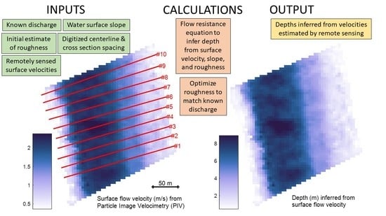
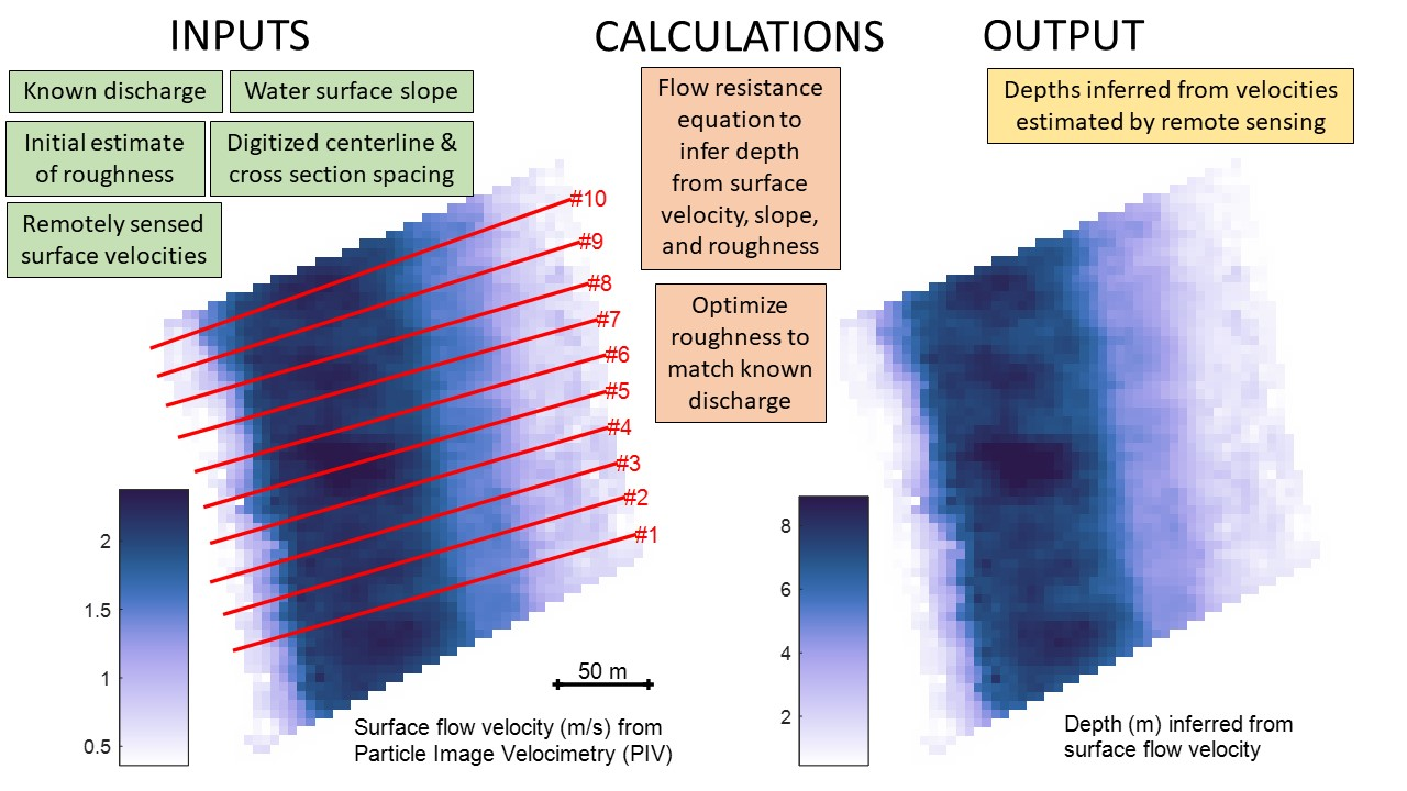
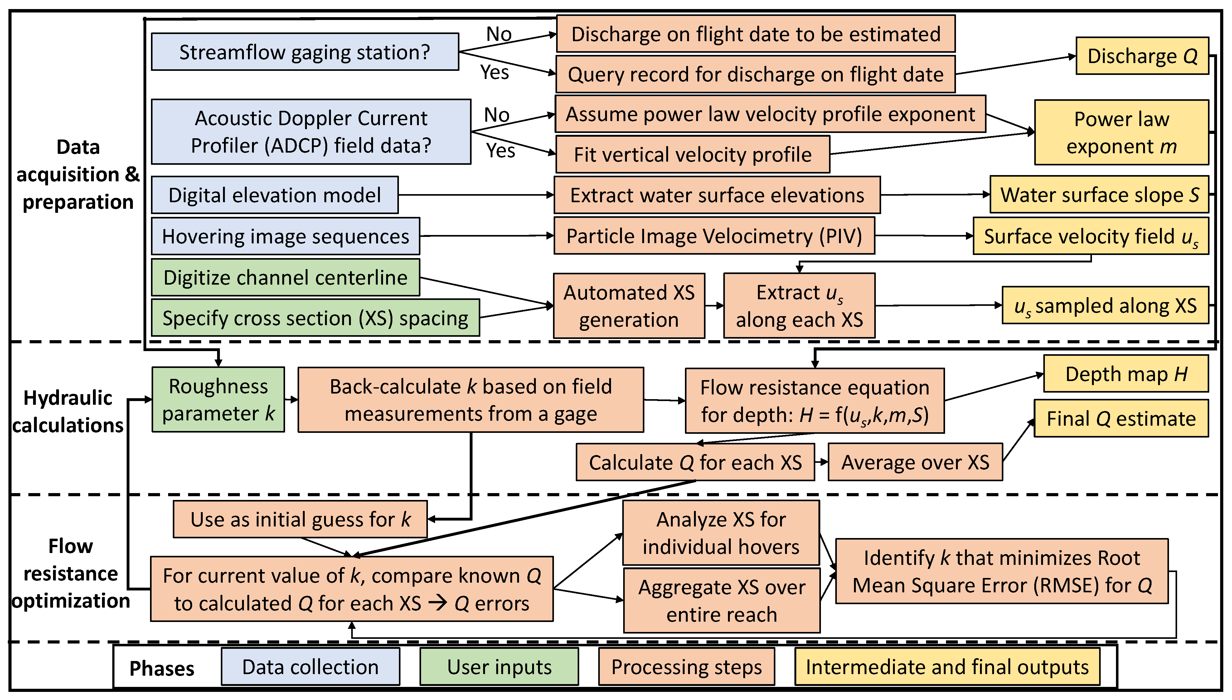
• Introduce the Depths Inferred from Velocities Estimated by Remote Sensing (DIVERS) framework for calculating depths from remotely sensed velocities via a flow resistance equation that expresses depth as a function of velocity, slope, and roughness.
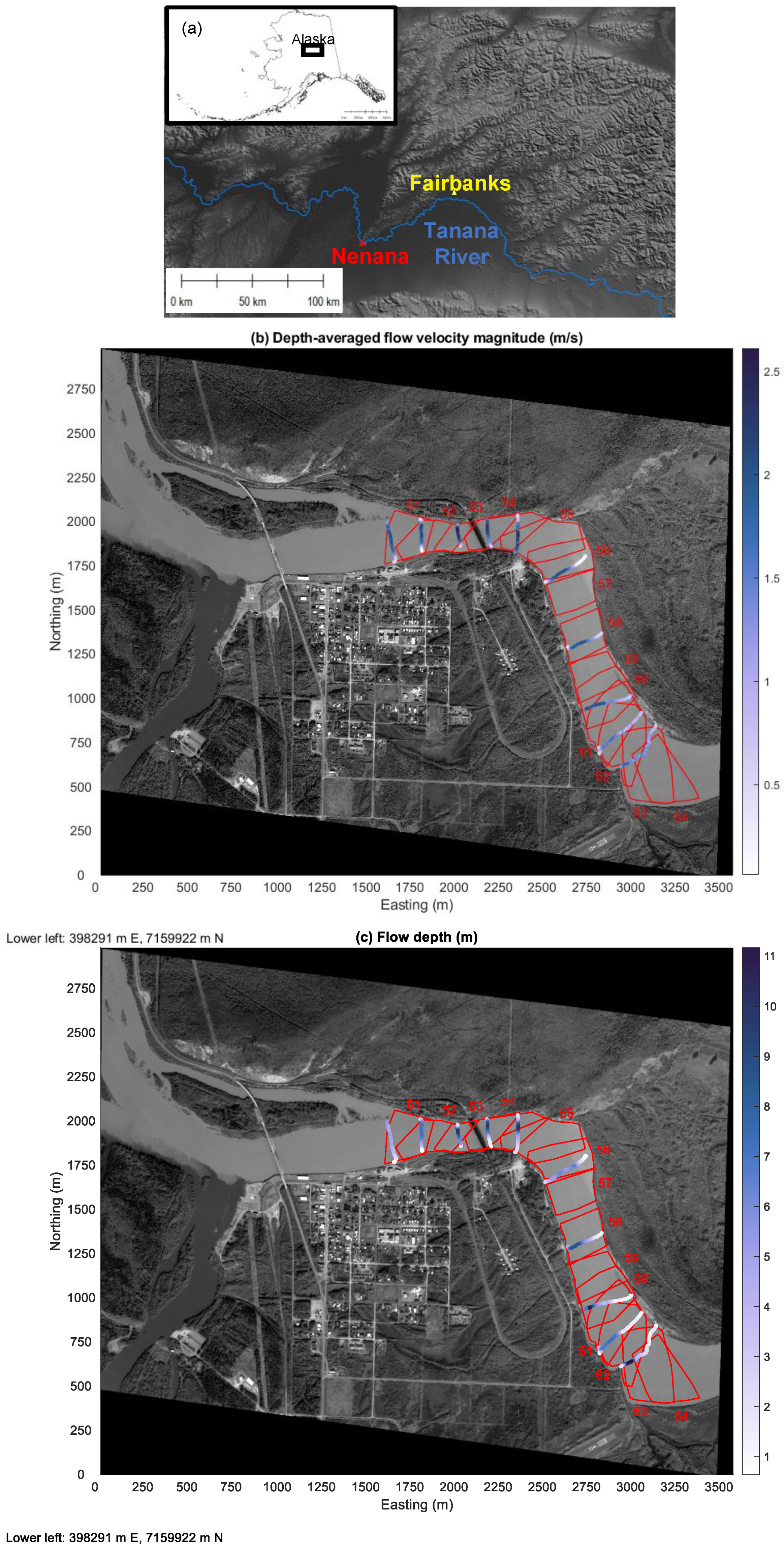
• Evaluate the potential of this approach by conducting a case study on a large, sediment-laden river in Alaska, the Tanana.
• Assess the suitability of a power law-based flow resistance equation for inferring depth from velocity by applying the relation directly to field measurements.
• Scale up a PIV-based workflow developed based on an image time series acquired from a helicopter hovering at a single location above the channel to a larger reach by applying the procedure to multiple hovers distributed along the river.
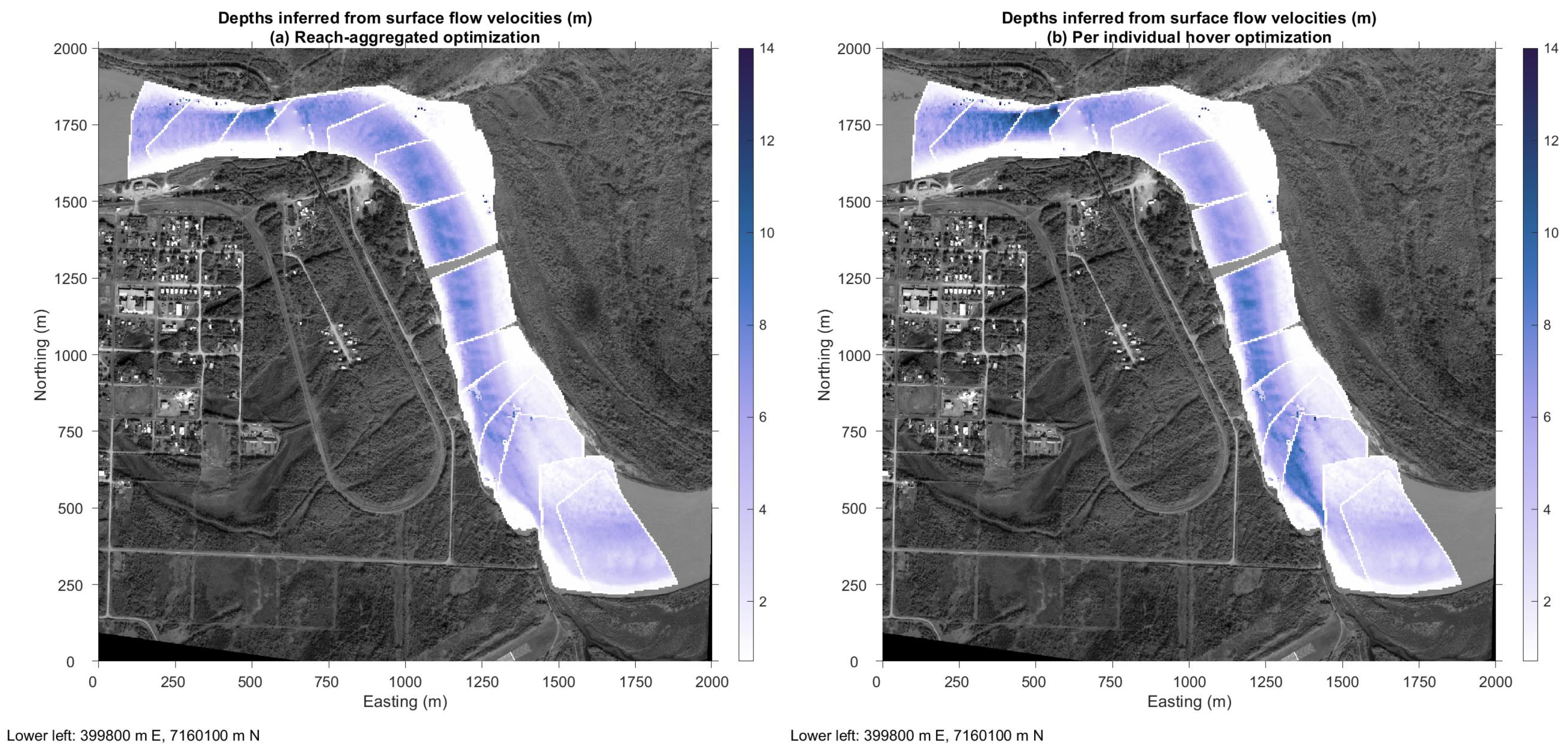
• Compare different methods of setting the roughness parameter, including per-hover or reach-aggregated flow resistance optimization (FRO) to match a known discharge.
• Quantify the accuracy of velocities, depths, and discharges inferred from remotely sensed data via comparison to field measurements.

2. Materials and Methods

The field measurements and remotely sensed data used in this study are publicly available via a data release hosted by the USGS ScienceBase catalog. Legleiter and Kinzel [22] provide a landing page with links to field measurements of flow depth and velocity and videos acquired from a helicopter.

2.1. Study Area

Alaska is the largest state in the USA and remains sparsely gaged due to the remote, inaccessible location of many of its rivers [1]. Non-contact methods of measuring river discharge are particularly valuable in this context and developing such techniques is an area of active research by the USGS. To support these ongoing efforts, this study focused on the Tanana River, a large, sediment-laden river typical of Alaskan waterways. Located southwest of the city of Fairbanks in the center of the state (Figure 1a), the 2.6 km reach examined herein was immediately upstream of the USGS gaging station at Nenana (#15515500), where the drainage area is 66,200 km${}^2$. The gage discharge on 24 July 2019, the date on which field observations and remotely sensed data were acquired, was 1722 m${}^3$/s, approximately the median of the mean daily values observed on this date over the 58 year period of record [23]. The water surface slope on this date was measured from a lidar DEM acquired the same day and was 0.00014.

The Tanana drains a large, glaciated watershed that delivers a steady supply of outwash and ensures consistently high concentrations of suspended sediment [24]. The presence of abundant suspended material within the water column is indicated by the bright tone of the Tanana River in the background satellite image shown in Figure 1b, whereas the more clear-flowing tributary entering from the south appears much darker. Legleiter and Kinzel [10] used 139 measurements of suspended sediment concentration (SSC) to establish a power function relating SSC to discharge; this expression yielded an estimated SSC of 2185 mg/L on the day the videos used in this study were obtained. More importantly, previous research at this site demonstrated that such high SSC allows surface flow velocities to be inferred under natural flow conditions, obviating the need to seed the flow with artificial tracer particles for PIV. This approach has a sound physical foundation: turbulence originating at the bed propagates upward through the water column to produce sediment boil vortices [25,26]. These ubiquitous features are expressed at the water surface as differences in color and brightness that can be tracked from frame to frame as they are carried downstream by the flow [10,27,28].

2.2. Remotely Sensed Data

As described in greater detail by Legleiter and Kinzel [10], the remotely sensed data used in this study consist of RGB (red, green, blue) videos acquired using a Zenmuse X5 camera [29] deployed from a Robinson R44 helicopter. This relatively basic, low-cost sensor was housed within an enclosure attached to the nose of the helicopter and mounted on a gimbal to improve stability. A remote control system allowed an operator onboard the helicopter to trigger the camera once the aircraft began hovering above each one of a series of 14 predefined waypoints distributed along the channel to provide reach-scale coverage. The videos/hovers were numbered sequentially from 51 to 64, increasing in the upstream direction (Figure 1b,c). The duration of the videos varied slightly among the 14 hovers but was at least one minute in all cases; all videos were truncated to 60 s. In total, acquisition of the videos used in this study spanned a period of 30 min. The flying height of the helicopter above ground level during data collection was $591\pm 3.9$ m. The original video files had a native frame rate of 30 Hz but we retained only every 30th frame based on the finding that reducing the frame rate to 1 Hz did not adversely affect the accuracy of PIV-based velocity estimates [10]. Because the Zenmuse camera was not integrated with a Global Positioning System/Inertial Motion Unit (GPS/IMU), the resulting image sequence could not be directly geo-referenced but did serve as suitable input to the workflow outlined by Legleiter and Kinzel [10] and summarized briefly in Section 2.4. Because the Tanana River was too deep and turbid to apply more traditional, spectrally based approaches to depth retrieval from passive optical data, we could not evaluate these methods as part of this study.

2.3. Field Data

We used direct field measurements of flow depth and velocity collected in situ on the same day as the helicopter flight to assess the accuracy of image-derived estimates of these two hydraulic attributes. The field data were collected within three hours of when the images were acquired during a period of steady discharge and thus were representative of the flow conditions captured in the videos. The field data were acquired with a TRDI RiverRay acoustic Doppler current profiler (ADCP) [30] that was integrated with a Hemisphere A101 differential GPS receiver that defined the location of each measurement with a horizontal precision of 0.6 m [31]. The ADCP was mounted on a small catamaran towed behind a boat while traversing the river along a series of ten cross sections (XS) oriented perpendicular to the mean flow direction. Each of these transects consisted of a single pass and spanned the full width of the channel. During field data collection, an operator in the boat controlled the RiverRay using TRDI WinRiver II software. This program enabled real-time visualization of the velocity field over the entire depth of flow as the boat traversed the river. The ADCP data were post-processed in WinRiver II, imported into the USGS Velocity Mapping Toolbox [32], and exported as a text file containing the easting and northing spatial coordinates, flow depth, and depth-averaged velocity magnitude at each measurement location.

For consistency with our previous work at this site and recent research by Pearce et al. [14], we used this simple summary of the ADCP data as is, without applying a velocity index [33] to convert depth-averaged velocities measured in the field to surface flow velocities that might have been more comparable to the velocities estimated via PIV. Instead, the DIVERS framework for inferring depths from image-derived velocities that is the primary focus of this study explicitly incorporates a site-specific velocity index to account for the difference between depth-averaged and surface velocities. As reported in greater detail by Legleiter and Kinzel [34], the value of this index was derived from the original ADCP data using the “extrap” module of the Qrev software package developed by the USGS [35,36]. The mean velocity index for the ten XS measured on the Tanana River was 0.88 and this value was used for all subsequent calculations.

2.4. Particle Image Velocimetry (PIV)

We derived spatially distributed velocity estimates from each of the 14 videos by following the PIV workflow established through previous research on the Tanana River. A more detailed description of this process was provided by Legleiter and Kinzel [10] and the interested reader is referred to the original publication for further information. This sequence of operations was implemented primarily within MATLAB and can be summarized as follows:

• Acquire video while hovering above the channel, select the frame rate to retain for analysis, extract the corresponding sequence of images, and convert the images from RGB to grayscale;
• Stabilize the image frames relative to one another to account for motion of the helicopter during acquisition. We used the TrakEM2 plugin [37] to the FIJI image processing package [38] for this purpose;
• Geo-reference the first image in the stabilized stack to a suitable base image. Tie points are used to define an affine transformation that is applied to each image to project the stack into a common real world coordinate system;
• Prepare the images for PIV by using FIJI to apply a finite Fourier transform bandpass filter and a histogram equalization contrast stretch;
• Extract the actual spatial footprint of each frame by outlining the boundary of the non-zero pixels in the image;
• Overlay the footprints of all the images in the stack to identify the area of common coverage and digitize a region of interest (ROI) for PIV;
• Crop all of the images in the stack to a common bounding box based on the digitized ROI and apply a binary raster mask to each image to obtain a series of co-registered, pre-processed, water-only images for PIV;
• Perform the PIV analysis using the ensemble correlation algorithm included within PIVlab, a widely used add-in to MATLAB developed by Thielicke and Stamhuis [39,40]. PIV settings to be specified by the user include the size (in pixels) of the interrogation area within which feature displacements are estimated by computing correlations between successive images and the step size that controls the spacing of the velocity vectors output from PIVlab. In this study, a fixed interrogation area of 64 pixels and a step size of 32 pixels was used to process all of the hovers;
• Post-process the PIV output by discarding spurious vectors that fall below a minimum velocity threshold, differ from the mean velocity magnitude by more than three standard deviations, or fail to pass a normalized median check [39]. To fill any gaps resulting from these filters and obtain continuous coverage, the remaining vectors are linearly interpolated;
• Scale the PIV output by using the ground sampling distance of the images (0.15 m in this study) to establish the number of pixels per meter and multiplying by the frame rate (1 Hz for this study) to obtain velocities in m/s. The geo-referencing information for the stack also is used to transform the vectors to the same real world coordinate system as the images.

Applying this workflow to the videos acquired at each of the 14 hovering locations along the Tanana River resulted in a set of spatially continuous, image-derived velocity fields. The filtered, interpolated PIV output vectors for each hover were used to produce regular grids of surface velocity magnitudes with a spacing of 4.8 m, the product of the image pixel size and the PIV step size parameter. These remotely sensed surface velocities were then used to infer flow depths via the DIVERS approach described next.

2.5. Depths Inferred from Velocities Estimated by Remote Sensing (DIVERS): A Flow Resistance Equation-Based Framework for Calculating Depth from Surface Velocity

The framework for estimating depths in addition to the velocities derived via PIV described herein is based upon a relatively simple flow resistance equation and predicated upon a number of critical assumptions. The assumptions involved in modeling flow and sediment transport in river channels, as well as their implications, are described in Nelson et al. [41]; only a few of particular relevance to this study are highlighted here. For example, the DIVERS approach approximates the flow field as steady, uniform, and one-dimensional, neglecting any flux of mass or momentum in the vertical or cross-stream directions. The flow is considered fully turbulent and treated as a boundary layer throughout the entire depth. However, rather than using the logarithmic velocity profile associated with a parabolic vertical distribution of eddy viscosity, the velocity profile is approximated by a more mathematically convenient power law formulation. Similarly, the flow is assumed to be hydrostatic so that the pressure gradient can be replaced by the water surface slope. The most significant assumption we make is that a flow resistance equation typically used to characterize bulk, cross-sectionally averaged (i.e., one-dimensional) hydraulics can be applied on a per-pixel basis to calculate local flow depths. This approximation allows velocity and depth to vary laterally from one node of the PIV output grid to the next across the channel, but each of these nodes is independent of those adjacent to it, with no information transferred from areas upstream, downstream, or to either side. In essence, each pixel is treated as an isolated water column and characterized via a one-dimensional, steady, uniform flow approximation. An important implication of this assumption is that secondary flows involving cross-stream currents such as those associated with meander bends are neglected. Moreover, our approach assumes strict proportionality between depth and velocity at a given location such that areas where the flow shoals and accelerates, as might occur over a point bar, or becomes deeper and slows down, as might occur within a pool, are not represented accurately. In addition to these spatial factors, we assumed that flow conditions were steady in time. For example, we did not consider temporal variations that might be associated with the passage of a flood wave and could lead to a hysteretic effect in the relationship between stage and discharge. The DIVERS framework thus offers, at best, a basic, first-order approximation to the actual hydraulic conditions present within a particular channel of interest.

With these assumptions and limitations borne in mind from the outset, the following derivation provides the basis for our approach to inferring water depths from remotely sensed velocities. Following Smart and Biggs [42], we begin with a power law velocity profile given by

$$\frac{u\left(z\right)}{u_{*}}=a{\left(\frac{z}{k}\right)}^m$$

(1)

where $u\left(z\right)$ is the flow velocity at a height z above the channel bed, $u_{*}$ is the shear velocity, k is a roughness length scale, and a and m denote a fitted (or assumed) coefficient and exponent, respectively. The velocity $u_s$ at the water surface, where $z=H$ and H represents the total flow depth, thus becomes

$$u_s=a{u}_{*}{\left(\frac{H}{k}\right)}^m$$

(2)

Similarly, integrating Equation (1) from the bed to the water surface and dividing by H yields the depth-averaged velocity U:

$$U=\frac{a{u}_{*}}{(m+1)}{\left(\frac{H}{k}\right)}^m$$

(3)

Smart and Biggs [42] also provide a parallel development for a specific, widely used flow resistance equation, Manning’s, which they show to be equivalent to a power law velocity profile with an exponent of $m=1/6$. In this study, we used Equation (1) for greater generality and to avoid dimensional issues associated with the roughness coefficient, n, used in Manning’s equation; k has units of length and thus a more readily interpretable physical basis.

In any case, taking the ratio of the depth-averaged velocity to the surface velocity yields a velocity index, $\alpha$, that is widely used to convert surface velocities derived from remotely sensed data to depth-averaged velocities e.g., [43]:

$$\alpha =\frac{U}{u_s}=\frac{1}{(m+1)}$$

(4)

The depth-averaged velocities needed to estimate discharge can thus be calculated as

$$U=u_s\alpha =\frac{u_s}{(m+1)}$$

(5)

To also infer the other hydraulic attribute required to compute river discharge, water depth, we next rearrange Equation (2) and make a substitution for the shear velocity: $u_{*}=\sqrt{gHS}$, where g is acceleration due to gravity and S is the water surface slope, to obtain an expression for depth H as a function of surface velocity $u_s$, slope S, and roughness k:

$$H={\left[\frac{k^m}{a\sqrt{gS}}{u}_s\right]}^{\frac{1}{\left(\frac{1}{2}+m\right)}}$$

(6)

In this study, we assume that the power law velocity profile given by Equation (1) adequately describes the flow at any location within the channel and, consequently, that Equations (5) and (6) can be used to derive the depth-averaged velocity and flow depth, respectively, from remotely sensed data. More specifically, in a spatial context, these two equations can be applied to each node (i.e., pixel) of a PIV output grid consisting of surface flow velocity magnitudes to produce a continuous map of depth.

To calculate the river discharge Q for a cross section extracted from the PIV output, we can then sum the resulting depth-velocity products laterally across the channel, assuming a uniform width increment $\Delta w$ between adjacent “verticals”:

$$Q=\Delta w\sum _{j=1}^N{U}_j{H}_j$$

(7)

where j indexes the N verticals along a cross section. Substituting Equations (5) and (6), we arrive at the following expression for discharge

$$Q=\Delta w\sum _{j=1}^N\left(\frac{1}{(m+1)}{u}_{s,j}\right){\left[\frac{k^m}{a\sqrt{gS}}{u}_{s,j}\right]}^{\frac{1}{\left(\frac{1}{2}+m\right)}}$$

(8)

This development provides a foundation for mapping water depth, by way of surface flow velocity, from remotely sensed data and, potentially, estimating river discharge. Image time series can be used to derive spatially distributed estimates of $u_s$ via PIV and water surface slope can be measured from a digital elevation model (DEM), which has become common practice and has been shown to provide water surface elevations with an accuracy comparable to conventional field methods (e.g., pressure transducers on rivers in Alaska [44]). The other variables in Equation (6) are the power law coefficient a and exponent m and the roughness parameter k. Ferguson [45] introduced a separate coefficient $a_1$, expressed U as a function of the median bed material grain size D rather than k, and assumed $m=1/6$ as in Manning’s equation to arrive at the following expression

$$U=a_1{u}_{*}{\left(\frac{H}{D}\right)}^{\frac{1}{6}}$$

(9)

Using a large compilation of field data, Ferguson [45] proposed a value of 7.5 for $a_1$. Equating (5) with (9) and letting $k=D$ yields a plausible, broadly applicable value of $a=6.43$. This approach is convenient because if one assumes a value of m, such as $1/6$ for Manning’s equation or $m=0.1765$ for the widely used default velocity index of $\alpha =0.85$, or calibrates m using measured velocity profiles e.g., [33,35,36], the only remaining unknown is the roughness parameter k.

Rather than specifying k a priori, remotely sensed surface velocities can be combined with measurements of Q made directly in the field or recorded at a gaging station and used to estimate k. This approach involves using an optimization algorithm to iteratively vary k so as to minimize the difference $ϵ$ between the measured discharge Q and the discharge $\widehat{Q}$ calculated from remotely sensed data via Equation (8) for a single cross-section

$$ϵ=Q-\widehat{Q}$$

(10)

For multiple cross sections, the objective function to be minimized becomes the root mean squared error (RMSE) between Q and $\widehat{Q_i}$ calculated for each of the $i=1,\dots ,M$ transects:

$$RMSE=\sqrt{\frac{1}{M}\sum _{i=1}^M{ϵ}_i^2}=\sqrt{\frac{1}{M}\sum _{i=1}^M{(Q-\widehat{Q_i})}^2}$$

(11)

Once k is calibrated in this manner, Equation (6) can be used to calculate H at each location of the PIV output grid and thus obtain a continuous map of flow depth to complement the surface velocity field derived via PIV.

2.6. Application to the Tanana River

Given this theoretical foundation and the assumptions described above, we evaluated the potential to infer water depths from remotely sensed surface velocities by applying the DIVERS workflow depicted graphically in Figure 2 to the Tanana River. For this case study, the inputs listed in the “Data acquisition and preparation” phase of the flowchart were obtained as follows. We queried the streamflow record for the USGS gaging station at Nenana to obtain the known discharge on the day the videos were acquired: $Q=1722$ m${}^3$/s. Similarly, we used ADCP data collected on the same date to fit vertical velocity profiles in Qrev and estimated the mean velocity index across the ten ADCP transects as $\alpha =0.88$. We then rearranged Equation (4) and used this value of $\alpha$ to calculate the power law exponent as $m=0.1364$; this value of m was assumed constant and used for all subsequent analyses. Water surface elevations were extracted from a lidar DEM that was acquired from the helicopter on the same day as the videos with a pixel size of 0.5 m and used to determine the water surface slope: $S=0.00014$. To obtain the transects of surface flow velocity $u_s$ required to calculate depth and discharge as outlined above, we digitized a channel centerline and used the automated procedure described by Legleiter [46] to extract cross sections from the velocity magnitude grids derived from the PIV output for each hover; the spacing between XS was set to 20 m, approximately 10% of the channel width.

For the “Hydraulic calculation” and “flow resistance optimization” phases of the workflow, we considered two different approaches: (1) using the known Q to identify the optimal value of k on a per-hover basis; and (2) aggregating XS over the entire reach by pooling across the hovers prior to the optimization of k to match the known Q. Hereafter, we refer to these two approaches as per-hover and reach-aggregated, respectively. The PIV workflow summarized above was applied in a consistent manner to provide a common set of input flow velocities to each approach for inferring water depth.

For both of these FRO-based approaches, we used MATLAB’s fminsearch routine as the optimization algorithm. This derivative-free method finds the minimum of an unconstrained multivariate function via the Nelder–Mead simplex search algorithm described in Lagarias et al. [47]. Using fminsearch required us to make an initial guess for k, the variable to be optimized. To obtain a plausible estimate of k, we back-calculated k from field measurements made during a site visit by USGS hydrographers to the gaging station at Nenana on the same day the videos were acquired. In addition to the official discharge reading, NWIS also reports the channel width, cross-sectional area, and mean flow velocity that were measured and used to compute the discharge. On 24 July 2019, these values were 211.5 m, 1059 m${}^2$, and $U=1.63$ m/s, respectively. We obtained the mean depth for the XS by dividing the area by the width: $H=5.01$ m. Substituting the depth-averaged velocity U for the surface velocity $u_s$ based on Equation (5) and rearranging Equation (6) then yielded an expression for k in terms of U and H:

$$k={\left[\frac{H^{\left(\frac{1}{2}+m\right)}a\sqrt{gS}}{U(m+1)}\right]}^{\frac{1}{m}}$$

(12)

Inserting the values of U and H derived from the field measurement at the gaging station into this equation, along with the values of m and S specified above, led to a value of $k=0.00054$ m for the known k approach. Our subsequent analysis indicated that the optimization algorithm was not highly sensitive to the initial guess for k.

2.7. Accuracy Assessment

To assess the accuracy of the velocity magnitudes and water depths inferred via PIV and the DIVERS framework, respectively, we compared the remotely sensed estimates to ADCP field measurements of depth-averaged velocity and depth. To make these comparisons, we used only those field observations located within a specified distance of a PIV output grid node. The search radius was set to 2.4 m, half the product of the step size in pixels, which dictated the spacing of the velocity vectors produced by PIVlab, and the image pixel size. This search strategy ensured that a given ADCP measurement would not be compared to multiple remotely sensed estimates. Where the search window encompassed several field measurements, all of the ADCP data within 2.4 m of the grid node were averaged to obtain a single value for comparison to the velocity and depth estimated at the center of the window [10].

After pairing the velocities and depths derived from the videos with those measured in situ by the ADCP, we computed several metrics for quantitative accuracy assessment. The root mean squared error (RMSE) provided an indication of the precision of the remotely sensed estimates while the mean bias served as an index of their absolute accuracy. The bias was calculated as the difference between the ADCP-measured velocities and depths and those derived from the videos. Given this definition, a positive value of the mean bias implied under-prediction, on average, of the ADCP-based observations by the PIV algorithm and DIVERS framework. Conversely, a negative bias implied that the velocities and depths inferred via remote sensing tended to exceed those measured in the field. We also normalized the RMSE and mean bias by by the mean of the ADCP measurements used to make the comparison to express these two metrics in non-dimensional terms as percentages of the mean velocity and depth [10].

In addition, we performed observed (ADCP) vs. predicted (PIV) (OP) regressions [48] and used the resulting $R^2$ values as a summary of the correspondence between the velocities and depths measured in the field and those obtained via remote sensing. The intercept and slope coefficients of the OP regression equations provided further information on the performance of the various image-based approaches we evaluated. For example, whereas an intercept of 0 and a slope of 1 would indicate perfect agreement, any deviation from these values would imply that the remotely sensed velocities and/or depths were biased (i.e., a non-zero intercept) or were not scaled correctly (i.e., a slope coefficient less than or greater than 1).

3. Results

3.1. Application of the Flow Resistance Equation to Field Measurements

As an initial test of the utility of the DIVERS framework for inferring water depths from observations of flow velocity described in Section 2.5, as well as the hydraulic assumptions inherent to the approach, we first applied DIVERS to the ADCP field data itself. More specifically, we used the depth-averaged velocities measured by the ADCP to predict the corresponding depths. These calculations involved making the substitution $u_s=U(m+1)$, per Equation (5), in Equation (6) and then using the measured values of U to solve for H. In performing these computations, we used the values of the water surface slope S and velocity exponent m given in Section 2.6. To specify the roughness, we used the k value back-calculated from the discharge field measurement made at the gaging station on the flight date.

The results of this analysis are summarized in Figure 3. An OP regression of the depths measured by the ADCP vs. those calculated from the corresponding velocity data via the flow resistance equation led to a modest $R^2$ value of 0.51 (Figure 3a). The large, positive intercept of the regression equation, 1 m, differed from the ideal value of 0 and indicated that the predicted depths were biased relative to the field measurements. Similarly, a slope coefficient less than 1 suggested that the depth estimates were not scaled correctly either. The distribution of depth estimation errors depicted in Figure 3b provided additional information on the discrepancies between the measured and calculated depths. The mean error of 0.37 m indicated that depths estimated via Equation (6) tended to under-predict the depths measured directly in the field. The standard deviation of these errors was 2.16 m, implying that the flow resistance-based framework did not provide precise depth estimates even when using in situ velocity observations as input. Moreover, the positive skew of the error distribution, with a long tail of large errors, in excess of 10 m in some cases, suggests that this approach could lead to major underestimates of depth.

The results presented in Figure 3 were based on ADCP data from throughout the entire reach, which encompassed a range of hydraulic environments.To minimize any potential confounding factors associated with river morphology, we performed a similar but more focused analysis that considered only those data from a single ADCP transect located in a straight section of the channel included within hover 58 (Figure 1b). In this case, a regression of measured vs. calculated depths produced a higher $R^2$ of 0.61 and a smaller, negative intercept term (Figure 4a). The regression slope coefficient remained less than 1 but was closer to this ideal value for the single transect case than when data from throughout the reach were used in the OP regression (Figure 3a). Although the mean depth estimation error of 1.53 m for the transect in hover 58 was larger than for the reach-aggregated data set, the standard deviation of the errors was less, 1.69 m vs. 2.16 m. However, the error distribution summarized in Figure 4b also featured a strong positive skew, with a secondary mode at 3.5 m and a maximum depth estimation error of over 5 m. As for the reach-aggregated case, these results implied that the flow resistance equation-based framework tended to underestimate the observed depths.

3.2. Image Stabilization and Geo-Referencing

The second and third steps in the PIV workflow summarized in Section 2.4 involved stabilizing and geo-referencing the image sequences. Co-registration errors associated with either or both of these processes could have introduced some degree of uncertainty into the subsequent PIV analysis and resulting velocity vectors. This possibility was examined in detail by Legleiter and Kinzel [10] for one of the hovers, 52, which we assumed to be representative of the other 13 hovers along the reach because all of the videos were acquired by the same sensor within a period of 30 min and were processed using a common workflow.

For hover 52, the TrakEM2 plugin used for image stabilization reported minimum, mean, and maximum displacement errors of 0.626, 0.853, and 1.069 pixels, respectively. For the 0.15 m ground sampling distance of this image sequence, these errors represented distances of 0.094, 0.13, and 0.16 m, respectively. Typical stabilization errors were less than the size of a single image pixel, which is the minimum distance a feature must move between frames to be detected by the PIV algorithm, and thus did not introduce significant uncertainty to the resulting velocity estimates.

Once stabilized, the image stack for each hover had to be geo-referenced so that PIV-derived velocities and inferred water depths could be compared to ADCP field measurements for accuracy assessment. For hover 52, we identified six tie points between the first image in the stack and the background satellite image, obtained via the Global Mapper software package [49], used as a base for geo-referencing. The affine transformation derived from these control points was used to predict the real world coordinates of the tie points from their (row, column) pixel coordinates in the Zenmuse image. Comparing these predictions to the actual spatial locations of the tie points on the base image led to a geo-referencing RMSE of 4.88 m. This error was uniform throughout the stack because the images had been stabilized relative to one another and the same transformation was applied to each frame.

Geo-referencing error did not influence the PIV output because the velocity estimates were based on relative displacements of water surface features between successive frames in the stabilized image sequence [10]. However, the absolute magnitude of the geo-referencing error could have affected the comparison of PIV-derived and ADCP-measured velocities. These two data sets were linked at a spatial resolution set by the cell size of the velocity magnitude grid produced from the PIV output, 4.8 m in this study. A typical geo-referencing error of 4.88 m thus was similar to the distance between PIV-derived velocity estimates, implying that the pairing of ADCP measurements with remotely sensed velocities and calculated depths might have been ambiguous in some cases. However, because these hydraulic attributes did not vary abruptly over distances on the order of 5 m on a river as large as the Tanana, we did not consider this type of geospatial error to be a major source of uncertainty.

3.3. Reach-Scale Mapping of Flow Velocities

The stabilized and geo-referenced image sequences for each hover were used to complete the remainder of the PIV workflow (steps 4–10 listed in Section 2.4). Whereas Legleiter and Kinzel [10] focused on a single hover, 52, during the initial development and testing of these procedures, this study assessed the potential to scale up the approach to map flow velocities over a longer river reach. This analysis involved producing a velocity field from the video acquired at each hover location, comparing the resulting PIV-derived velocity estimates to the ADCP field measurements located within that particular hover, and calculating the metrics of performance described in Section 2.7. Two of the hovers, 57 and 59, did not encompass any of the ADCP transects and quantitative accuracy assessment thus was not possible for these subsets of the reach.

The results for the other hovers are summarized in Figure 5 and

Table 1. Summary of accuracy assessment of PIV-derived surface flow velocity estimates via comparison to ADCP field measurements. n is the number of ADCP data points within each hover; OP = observed vs. predicted; int. = intercept; RMSE = root mean squared error; Norm. = normalized (by the mean of the field measurements within the hover).

Hover	n	OP ${\mathit{R}}^2$	OP int.	OP Slope	Bias (m/s)	RMSE (m/s)	Norm. Bias	Norm. RMSE
51	81	0.898	0.079	0.989	−0.062	0.222	−0.041	0.147
52	60	0.869	0.179	0.888	0.018	0.227	0.010	0.129
53	61	0.549	−0.390	1.091	0.223	0.563	0.121	0.305
54	70	0.390	0.614	0.667	−0.022	0.452	−0.012	0.254
55	26	0.547	0.549	0.639	0.184	0.258	0.090	0.127
56	48	0.974	0.194	0.994	−0.187	0.231	−0.164	0.202
57	0
58	43	0.926	0.221	0.945	−0.145	0.215	−0.105	0.156
59	0
60	56	0.887	0.107	0.983	−0.081	0.185	−0.056	0.128
61	118	0.381	0.437	0.764	−0.154	0.468	−0.129	0.390
62	93	0.502	0.179	0.992	−0.170	0.373	−0.136	0.300
63	62	0.599	−0.070	1.049	0.008	0.220	0.007	0.176
64	29	0.221	0.514	0.539	0.082	0.202	0.064	0.157
Median	58	0.574	0.187	0.964	−0.042	0.229	−0.027	0.166

. The OP regression $R^2$ varied from 0.22 to 0.97, with a median value of 0.57 across the 12 hovers. Correspondence between the velocities observed in the field and those predicted from the remotely sensed data was quite strong at the downstream end of the study reach (hovers 51 and 52) but then weakened for hovers 53–55. Farther upstream, the OP $R^2$ reached its highest value for hover 56 (0.97) and was nearly as high for hovers 58 (0.93) and 60 (0.89). The agreement between ADCP-measured and PIV-derived velocities presumably was also strong for hovers 57 and 59, but no field data were collected within the footprints of these two image sequences. At the upstream end of the study area, the OP $R^2$ values decreased.

The other metrics of accuracy and precision also varied spatially from hover to hover throughout the reach. The bias of the PIV-derived velocity estimates relative to the ADCP field measurements ranged from −0.17 m/s to 0.22 m/s across the hovers, with a median value of −0.04 m/s. When scaled by the mean of the field measurements within each hover, these values correspond to normalized mean biases from −13.6% to 12.1%, with a median of −2.7%, indicating that PIV provided accurate velocity estimates. Moreover, Figure 5 shows that velocities derived from remotely sensed data did not consistently under-or over-predict depth-averaged velocities observed in the field.

The precision of the remotely sensed velocities was quantified in terms of the RMSE relative to the ADCP measurements. The RMSE varied from 0.19 m/s to 0.56 m/s among the 12 hovers for which field data were available for accuracy assessment, with a median of 0.23 m/s. When normalized by the mean of the measured velocities within each hover, these minimum, maximum, and median values were 12.7%, 39%, and 16.6%. The spatial variation of the RMSE generally mirrored that of the OP $R^2$ metric discussed above, with lower RMSE values for hovers 51 and 52 at the downstream end of the reach as well as hovers 58 and 60 in the section between the two meander bends. Conversely, larger errors occurred for hovers 53, 54, 61, and 62, locations which also had low OP $R^2$ values. However, some locations with high OP $R^2$ values had relatively large RMSE (e.g., hover 56), whereas other areas with very low OP $R^2$ values did not have unusually high RMSE (e.g., hover 62). These discrepancies were a consequence of the number of field measurements located within each hover and their variability. ADCP transects that captured a small range of velocities could lead to low OP $R^2$ values and yet have relatively small RMSE. In any case, the remotely sensed velocities derived via PIV provided the input required to infer water depths using the DIVERS workflow.

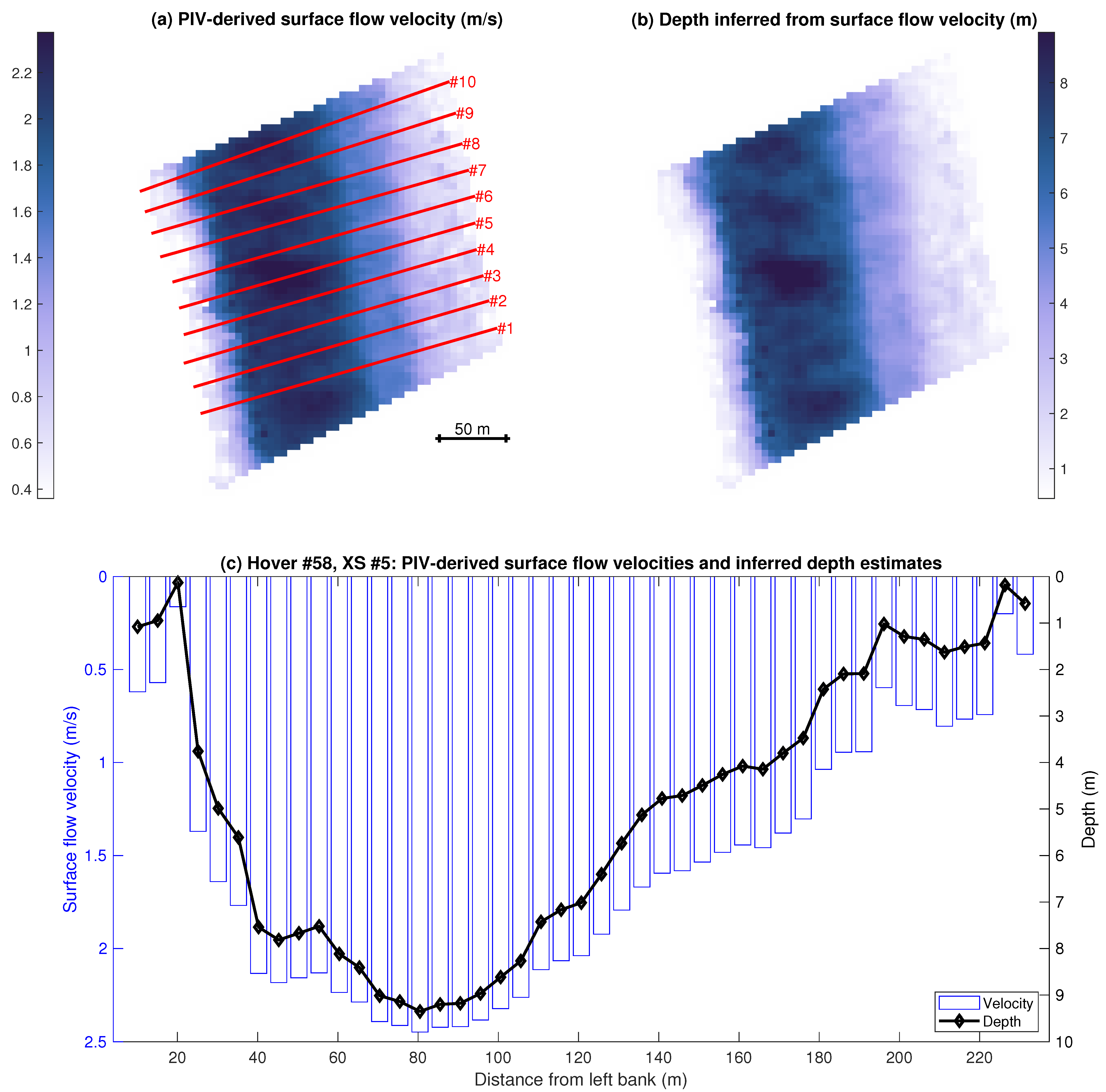
3.4. DIVERS Output from a Single Hover

To illustrate the inputs to and outputs from the DIVERS framework, we selected a single hover, produced maps of velocity and depth, and plotted a transect showing how the estimated depths and velocities varied laterally across the channel (Figure 6). Although we highlighted hover 58 as a representative example because this video captured a straight reach of the channel and included an ADCP transect that encompassed a broad range of velocities and depths, similar analyses were conducted for all of the other hovers as well. The velocity field depicted in Figure 6a was produced via the PIV workflow summarized in Section 2.4 and features higher surface velocities, up to 2.3 m/s, near the left bank.We digitized a centerline on the PIV map and used an automated procedure [46] to generate the 10 XS shown in Figure 6a. The surface velocities extracted from the PIV output along each of these transects served as input to the DIVERS framework, along with the known discharge and water surface slope listed in Section 2.6. For the case illustrated in Figure 6, we optimized the roughness parameter k using only the XS within this particular hover (i.e., the per-hover FRO approach). As an initial guess for k, we used the value back-calculated from the discharge field measurement made on the flight date. Given these inputs, implementing the workflow represented in Figure 2 led to the depth map shown in Figure 6b. The greatest predicted depths, over 9 m, occurred on the left side of the channel, with much shallower water to the right of the centerline.

The relationship between velocity and depth became even more evident when examined in a cross-sectional plane, as illustrated in Figure 6c. The surface velocities derived from the hover 58 video via PIV are represented by blue bars and the depths inferred from these velocities via Equation (6) are depicted by the black line. The two plots closely parallel one another, with the greatest predicted depths occurring 80 m from the left bank where the surface velocities are fastest. Conversely, slower flow less than 1 m/s, at cross-stream distances greater than 180 m translated into shallower depth estimates less than about 3 m. Each subtle variation in the PIV-derived velocity field, such as the locally lower values of $u_s$ 20 and 190 m from the left bank, translate into positive features in the inferred bottom profile.

An accuracy assessment of the depths inferred from the remotely sensed data by way of the PIV-derived surface velocity field for hover 58 is summarized in Figure 7. Comparison of the calculated depths with those measured in the field via OP regression indicated fairly strong agreement, with an $R^2$ value of 0.78, much higher than when depths were predicted directly from field measurements of velocity ($R^2=0.61$; Figure 4a). Moreover, the intercept of the regression equation in Figure 7 was only slightly less than 0 and the slope coefficient was closer to 1, implying that the depths derived from remotely sensed data were nearly unbiased and properly scaled. Similarly, the distribution of depth estimation errors has a mean of 0.67 m, less than half that based on the ADCP data (Figure 4b), as well as a smaller standard deviation (1.2 m for remote sensing vs. 1.69 m for the ADCP). The error distribution again is positively skewed, with a tail of relatively large positive values indicating under-predictions of depth from the remotely sensed data. Overall, however, these results suggest that, at least on a per-hover basis and for this particular hover, the DIVERS approach proposed herein was capable of providing bathymetric information that was as accurate as, if not to superior to, that obtained by applying the flow resistance equation to field measurements of velocity. We attribute this surprising result to the coarse spatial resolution of the remotely sensed data, with a PIV output grid node spacing of 4 m, relative to the point measurements from the ADCP, which thus provided a much larger sample size. Also, whereas the image-based analysis produced depth estimates that were evenly spaced across the channel, the ADCP data might have included more points in some areas where the boat was moving more slowly, such as along the east bank where the depths recorded by the ADCP were much greater than those calculated from the velocity measurements via the flow resistance equation; these points are represented on the right side of Figure 4a. In any case, the key finding is that the DIVERS framework yielded reasonably accurate depth estimates when applied to remotely sensed data.

To gain further insight on this approach and provide some more intuitive, graphical representation of the FRO process, we analyzed the sensitivity of the predicted depths and discharges to the roughness parameter k for hover 58. As illustrated in Figure 2, our workflow involved identifying the value of k that led to the best match between the discharges predicted from the PIV output via Equations (6) and (8) and the known discharge specified as input. An initial guess for k also must be specified and in this study we used a value of 0.00054 m, or 0.54 mm, back-calculated from the field measurement made by USGS hydrographers at the Nenana gage on the day of the flight. Given this starting point, the fminsearch optimization algorithm iteratively adjusted k so as to minimize the objective function, the discharge RMSE given by Equation (11). An additional output from this procedure is the optimal k, which was 1.29 mm for hover 58, more than twice our initial guess. Despite this large discrepancy between the initial and optimal values of k, the fminsearch algorithm converged and nearly reproduced the known discharge of 1722 m${}^3$/s, with a mean discharge of 1714 m${}^3$/s averaged over the 10 XS used as input; the corresponding value of the objective function was an RMSE of 115 m${}^3$/s.

For the sensitivity analysis, we used k values ranging from half to twice the optimal value in Equations (6) and (8) to calculate depths and discharges for each value of k. The discharge error and RMSE and the normalized mean bias and RMSE of the resulting depth estimates were then plotted as a function of k (Figure 8). This graphical representation provided a glimpse into the parameter space explored by the fminsearch optimization algorithm and confirmed that the optimal k of 1.29 mm resulted in the closest match to the known discharge, within 1.5% (Figure 8a), and the smallest discharge RMSE, 6.7% of the known discharge (Figure 8b). Values of k less than the optimum led to larger positive discharge errors, indicating under-prediction of the known discharge, and correspondingly greater RMSE. Conversely, as k increased beyond the optimal value of 1.29 mm, the discharge error became negative, implying over-predictions, and the RMSE began to increase again after reaching its minimum.

Another important input to the flow resistance equation is the water surface slope S, which in this study was calculated based on water surface elevations extracted from a lidar DEM acquired on the same day as the videos and field observations. Measurements of S are subject to some degree of uncertainty, however, particularly for the more typical situation where lidar data are not available and elevations must be extracted from a coarser, presumably less accurate DEM. To assess the potential impact of any errors in S on the discharges and depths inferred via DIVERS, we performed a sensitivity analysis analogous to that for k, again focusing on hover 58. For the slope sensitivity analysis, we held k fixed at the optimal value of 1.29 mm and varied the input S from one half to twice the slope derived from the lidar DEM, 0.00014. The same four error metrics examined in the k sensitivity analysis were calculated and plotted as a function of S (Figure 9). This analysis indicated that using the water surface slope measured from the lidar DEM led to the smallest discharge error (1.5%) and minimized the discharge RMSE (6.7%). If a smaller value of S were used as input, larger underestimates would have occurred, with an error of −71% and RMSE of 72% for a slope that was half the measured value. For input values of S that were too steep, the discharge was less sensitive to S but was overestimated by 42% for an S twice as large as that measured from the lidar DEM. Depth estimation errors followed a similar pattern, with increasingly large underestimates for water surface slopes less than the true value and overestimates for values of S that were too large. The normalized RMSE of the depth estimates reached a minimum of 24% for an input water surface slope of 0.000126, 10% less than that measured from the lidar DEM, but increased for smaller or larger values of S.

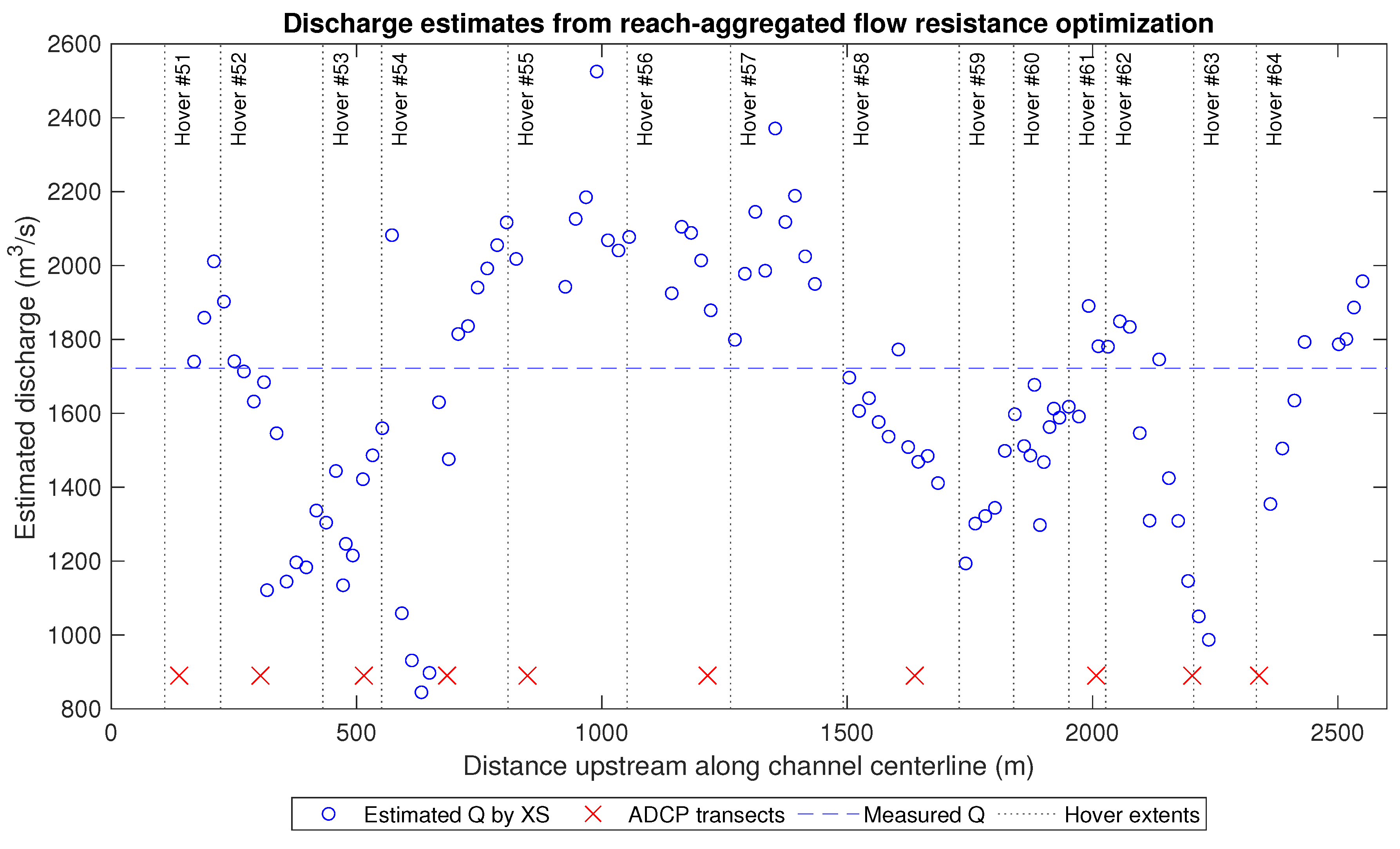
3.5. Reach-Aggregated Flow Resistance Optimization

The results presented in the previous section were produced by applying the FRO version of the DIVERS workflow to a single hover using only the XS extracted from the PIV-derived velocity magnitude grid for that particular hover. As an alternative to this type of per-hover analysis, we also considered a reach-aggregated approach in which XS from all of the hovers were pooled together and the resulting compilation used as input to the optimization algorithm. The spatial footprints for several of the hovers crossed the channel at an oblique angle, rather than being perpendicular to the mean flow direction as would have been the ideal geometry. As a result, we could not use a single centerline for the entire reach to automatically generate XS because many of the transects would not have extended across the full channel width, which was essential for the discharge calculation that is a central component of the DIVERS framework. Instead, we ensured that all XS spanned the entire channel by digitizing a centerline and extracting XS separately for each hover before aggregating them over the reach.

This process resulted in a total of 104 XS distributed across the 14 hovers as shown in Figure 10. Also indicated on this figure are the along-channel locations of the centroids of the ten ADCP transects. Pooling the XS for input to the optimization led to a single estimate of the roughness parameter k for the entire reach, 0.001 m, and using this value in Equations (6) and (8) yielded a discharge estimate for each XS. The calculated values of Q varied considerably throughout the reach, from as little as 800 m${}^3$/s to nearly 2600 m${}^3$/s, but the mean value of 1650 m${}^3$/s was within 4.2% of the discharge recorded at the gaging station on the day of the flight. These results indicate that although the discharge estimated at any one of the XS extracted from the PIV-derived velocity fields might not be highly reliable, pooling the XS over the entire reach yielded a more accurate mean discharge estimate.

Given the single value of k inferred via FRO for the entire reach, Equation (6) provides a means of inferring a flow depth at every node of the PIV output grid for each hover. An accuracy assessment of the depths calculated via this approach is summarized in Figure 11. For the reach-aggregated compilation of estimated depths, the OP $R^2$ value of 0.45 was much lower than that for hover 58, presented above (Figure 11) as an example of the per-hover version of the DIVERS framework. The OP regression equation intercept of 1.69 indicated that the image-derived depth estimates were biased and a slope coefficient of 0.539, well below the ideal value of 1, implied that the depths were not scaled correctly, either. The histogram of depth estimation errors depicted in Figure 11b corroborated these results. A mean error of 0.46 m indicated that the calculated depths tended to underestimate those measured directly in the field, but the median error was only 0.01 m because the distribution was positively skewed, with a long tail of very large under-predictions up to 10.2 m. The standard deviation of the errors was 2.21 m, suggesting that the reach-aggregated approach did not yield precise depth estimates. The normalized mean bias and RMSE for this version of the DIVERS workflow were 10% and 48.3%, respectively, of the mean depth observed in the field.

3.6. Accuracy Assessment Summary and Comparison of Approaches

The performance of the two FRO-based variants of DIVERS is summarized in Figure 12. The strength of the association between the calculated depths and the ADCP field measurements was summarized in terms of the OP regression $R^2$ and was higher for the per-hover than for the reach-aggregated FRO for 8 of the 12 hovers for which ADCP data were available. The more detailed information presented in

Table 2. Summary of accuracy assessment of depths inferred from surface flow velocity estimates via comparison to ADCP field measurements for the two approaches evaluated in this study. n XS is the number of cross sections extracted from each hover; n is the number of ADCP data points within each hover; OP = observed vs. predicted; int. = intercept; RMSE = root mean squared error; Norm. = normalized (by the mean of the field measurements within the hover.

Hover	k Method	n XS	Fit k (m)	n	OP ${\mathit{R}}^2$	OP int.	OP Slope	Norm. Bias	Norm. RMSE
51	Per-hover	8	0.000708	84	0.751	−0.636	1.101	0.039	0.277
52	Per-hover	9	0.003242	61	0.627	−0.779	1.247	−0.122	0.358
53	Per-hover	9	0.002227	64	0.758	−0.624	1.131	−0.024	0.330
54	Per-hover	10	0.000619	70	0.430	2.436	0.481	0.086	0.384
55	Per-hover	7	0.000303	26	0.400	3.097	0.349	−0.152	0.338
56	Per-hover	5	0.000420	48	0.614	−1.207	1.019	0.249	0.430
57	Per-hover	9	0.000359
58	Per-hover	10	0.001289	44	0.783	−0.016	0.878	0.125	0.254
59	Per-hover	10	0.001803
60	Per-hover	9	0.001078	56	0.634	2.284	0.553	−0.125	0.495
61	Per-hover	6	0.001062	118	0.425	1.360	0.694	−0.083	0.573
62	Per-hover	4	0.005958	93	0.320	3.364	0.458	−0.104	0.594
63	Per-hover	4	0.001248	62	0.536	2.268	0.264	0.161	0.772
64	Per-hover	4	0.000597	29	0.597	1.038	0.642	−0.056	0.209
Median	Per-hover	8.5	0.001070	62	0.606	1.199	0.668	−0.040	0.371
Aggregated	Reach-agg.	104	0.001	712	0.452	1.691	0.539	0.099	0.483

also indicated that the intercept and slope terms in the OP regression equations differed between the per-hover and reach-aggregated FRO approaches. The intercept was typically closer to 0 and the slope closer to 1 for the per-hover FRO than for the reach-aggregated version, implying that performing the optimization on a per-hover basis tended to lead to depth estimates that were less biased and scaled more appropriately. However, even when optimized for each hover, the intercept and slope coefficients were far removed from the ideal values of 0 and 1, respectively, that would occur if agreement between observed and predicted depths were perfect.

Considering the distributions of the depth estimation errors for the different versions of DIVERS provided additional insight. Scaling the errors by the mean of the field-measured depths within each hover and computing their average to obtain the normalized mean bias indicated that the per-hover FRO approach led to less biased estimates of depth, with a median value of −4%, whereas reach-aggregated FRO yielded a mean bias of 10%. These results suggest that depths tended to be slightly over-predicted for the per-hover FRO approach but under-predicted for the reach-aggregated approach. However, examining the variation of the bias from hover to hover along the reach (Figure 12) revealed that this metric fluctuated among the hovers and that in most cases (hovers 51–54 and 56–63) the per hover FRO approach led to negative biases; and biases were positive for only two of the 12 hovers with ADCP data (55 and 64). In addition, the normalized RMSE provided a metric of the precision of the depth estimates generated by the two different implementations of DIVERS. For the individual hovers, the per-hover FRO approach had RMSE values that tended to be greater for per-hover FRO (median of 37%)than for reach-aggregated FRO, which led to less precise depth estimates with an RMSE of 48%.

In addition to the depth accuracy assessment, we also compared the two DIVERS approaches in terms of their ability to reproduce the known discharge recorded at the USGS gaging station on the day the images were acquired. Errors were defined as the difference between the discharge measured at the gage and the mean of the discharges calculated for each of the cross sections extracted from the PIV output grids. Similarly, the discharge RMSE was computed using Equation (11). The results of this analysis are summarized in Figure 13 and

Table 3. Summary of accuracy assessment of discharges inferred from surface flow velocity estimates via comparison to the known discharge of 1722 m³/s measured at the gaging station for the two approaches evaluated in this study. Errors are calculated as known minus estimated. n XS is the number of cross sections extracted from each hover; RMSE = root mean squared error; Norm. = normalized (by the known discharge).

Hover	k Method	XS	Q error (m${}^3$/s)	Q RMSE (m${}^3$/s)	Norm. Error (%)	Norm. RMSE (%)
51	Per-hover	8	7.63	114.44	0.44	6.65
52	Per-hover	9	18.78	179.69	1.09	10.44
53	Per-hover	9	121.75	457.99	7.07	26.60
54	Per-hover	10	63.71	331.29	3.70	19.24
55	Per-hover	7	11.07	138.55	0.64	8.05
56	Per-hover	5	3.32	76.20	0.19	4.43
57	Per-hover	9	9.74	129.44	0.57	7.52
58	Per-hover	10	7.70	115.35	0.45	6.70
59	Per-hover	10	17.90	175.50	1.04	10.19
60	Per-hover	9	18.22	176.75	1.06	10.26
61	Per-hover	6	27.37	217.22	1.59	12.61
62	Per-hover	4	19.85	184.85	1.15	10.73
63	Per-hover	4	18.04	176.28	1.05	10.24
64	Per-hover	4	2.33	63.88	0.14	3.71
Median	Per-hover	8.5	17.97	175.89	1.04	10.21
Aggregated	Reach-agg.	104	71.99	352.04	4.18	20.44

. The accuracy of the discharge estimates varied considerably from hover to hover but in almost all cases was significantly better for the per-hover FRO approach than for the reach-aggregated version. The precision of the discharges inferred via the various DIVERS workflows, as indexed by the RMSE of the discharges calculated for the individual XS, also fluctuated from hover to hover within the reach (Figure 13). Attempting to match a known discharge by applying the FRO algorithm on a per-hover basis led to the smallest RMSE values, ranging from less than 4% for hover 64 to 27% for hover 53, with a median of 10% (Table 3). Aggregating the XS over the entire reach before applying the FRO technique more than doubled the RMSE of the estimated discharges, to over 20%.

4. Discussion

4.1. A Field Test of the DIVERS Framework

The motivation for the analysis summarized in Section 3.1, in which the DIVERS framework was applied to field data collected with an ADCP, was to evaluate the degree to which the relatively simple approach outlined in Section 2.5 could be used to relate depth and velocity when both attributes were measured directly in the field, without the complications and uncertainties introduced by estimating velocities from remotely sensed data. By instead inferring depth from in situ velocity observations, we sought to assess the potential to apply this framework in a remote sensing context, identify the limitations of the approach, and establish realistic expectations.

Initially, we considered ADCP data from the entire reach, which led to a modest OP $R^2$ of 0.51 and many large underestimates of depth (Figure 3). However, aggregating field observations from throughout the study area, which included both relatively simple hydraulic settings as well as more complex areas (e.g., meander bends with pronounced secondary flow patterns), obfuscated the effects of channel morphology on the performance of the DIVERS framework. To reduce these complications and facilitate interpretation, we also performed a separate analysis focused on a single ADCP transect in a straight section of the channel within the footprint of the hover 58 video. Although comparing the DIVERS-based depth estimates for this cross section to those measured in the field resulted in a higher OP $R^2$ of 0.61 and less variable errors, depths still tended to be underestimated (Figure 4).

To gain further insight regarding these errors, we also examined their spatial distribution by plotting depth estimation errors in the context of the cross section along which the data were collected. The map presented in Figure 14 revealed that the calculated depths agreed closely (i.e., errors near 0) with the field measurements toward the right bank and in the center of the channel, with a few locations where the predicted depths exceeded the observations, as represented by the blue point symbols. However, to the left of the channel centerline, and especially near the left bank, applying Equation (6) to the velocity measurements led to large underestimates of depth, up to 5 m shallower than the depths recorded by the ADCP in this area.

Taking a broader perspective on the study reach by reexamining Figure 1c showed that the river’s bathymetry was strongly asymmetric in the vicinity of hover 58, with greater depths along the left side of the channel and much shallower flow over a bar on the right. This morphology was a consequence of the meander bend at the upstream end of our study area, which led to faster, deeper flow along the outer (left) bank that persisted well downstream of the bend apex, including the area covered by hover 58 and depicted in Figure 14. As a result of the flow field inherited from upstream, the ADCP transect we examined was strongly influenced by secondary (i.e., cross-stream) flows that were not incorporated into the simple flow resistance equation based solely on velocity magnitude, not along- and across-stream components. These results indicate that omitting such effects limited the predictive ability of Equation (6), even when using field measurements of velocity to estimate flow depths. Moreover, the low OP $R^2$ values and large, positively biased depth estimation errors obtained when using only in situ observations imply that the accuracy of depths from inferred remotely sensed surface velocities could be constrained by the inherent deficiencies of the flow resistance equation at the core of the DIVERS framework.

4.2. Spatial Variations in Performance and Limitations of the Flow Resistance Equation

The results summarized in Figure 5 and Table 1 indicated significant along-reach variability in the performance of the DIVERS framework and served to highlight some important limitations of the approach. For example, although agreement between depths measured directly in the field and those inferred from remotely sensed data was strong at the lower end of the reach (hovers 51 and 52), the OP $R^2$ decreased for hovers 53–55. This deterioration might reflect the presence of a railroad bridge that created artifacts during image processing and/or a more complex flow field where the channel curved to the west (Figure 1b,c). We observed further evidence of the influence of channel morphology on the accuracy of DIVERS-based depth estimates at the upstream end of the study area, where the OP $R^2$ values decreased as the flow field was influenced by another meander bend, this time where the river began flowing to the north.

The effects of the fluvial processes operating within this sinuous channel on the performance of the DIVERS framework were also expressed at a more local scale. For example, in the more detailed analysis of the output from a single hover presented in Section 3.4, the pattern of bathymetry illustrated in Figure 6b mirrored that of the velocity field in Figure 6a and was a reflection of meander-related flow structure. As a result of the complex hydraulics in this area, the largest underestimates of depth occurred on the left side of the channel where the river was deepest and the flow resistance equation failed to account for secondary flows associated with meandering, as described above in the context of Figure 14.

The similarity between the maps of velocity and depth shown in Figure 6 is a consequence of Equation (6), which summarizes a direct proportionality between H and $u_s$. Although this expression is not linear, for the value of m used in this study, the exponent on $u_s$ is 1.57, so the relation is only weakly non-linear. As a result, differences in predicted depth closely track fluctuations in the PIV-derived velocity field. Moreover, because Equation (6) is applied in an aspatial manner on a per-pixel basis, without reference to nearby velocities, the depth inferred at a given location depends exclusively on the remotely sensed surface velocity at that same location. In essence, therefore, the flow resistance equation merely serves to convert the velocity field into a depth map without any significant modification of the spatial pattern generated by the PIV algorithm. An important implication of these results is that the simple, flow resistance equation-based DIVERS framework cannot account for more complex hydraulics where the local depth does not scale with the local velocity, as might occur near the inner bank above the apex of a meander bend where the flow shoals and accelerates over a point bar to produce a higher velocity but a shallower depth.

In addition, the sensitivity analysis to the roughness parameter k presented in Section 3.4 revealed further limitations of the flow resistance equation-based approach outlined herein. Considering the influence of k on the predicted depths provided a plausible physical explanation for the results summarized in Figure 8. For lower values of the roughness coefficient k, the flow resistance due to friction against the channel boundary was reduced and a given discharge could be conveyed with a shallower depth, given the same velocity. As a result, depths tended to be under-predicted for low values of k, as indicated by the large positive normalized mean bias values on the left side of Figure 8c. As k increased, however, the flow resistance became greater and the conveyance of a given discharge was accomplished with greater depths for a given velocity. Depths were thus under-predicted to a lesser degree, resulting in lower values of the normalized mean bias for larger k in Figure 8c. For the greatest k values considered in this sensitivity analysis, depth estimation errors approached 0 and then became slightly negative, implying that depths might be over-predicted if the roughness used in Equation (6) were too high. Similarly, the normalized depth RMSE decreased as k increased, even for k values larger than that identified as optimal by minimizing the discharge RMSE (Figure 8d). In this case, a slightly greater k of approximately 1.8 mm would have minimized the normalized RMSE of the depth estimates. These results suggest that optimizing the roughness so as to match the known discharge might not lead to the most accurate depth estimates because discharge depends not only on depth but also velocity.

The sensitivity analysis to water surface slope summarized in Figure 9 also provided insight on the influence of uncertainty in this important input parameter on estimated discharges and depths. As for the effects of k described above, these results could be interpreted in terms of the associated physical processes. For S values that were too gentle, the flow resistance equation led to underestimates of depth (large negative values on the right side of Figure 9c) for a given velocity and thus negative discharge errors (right side of Figure 9a). Conversely, if the input slope were too steep, depths calculated via Equation (6) would be too high, leading to a positive mean bias for depth and an overestimate of the discharge (left side of Figure 9a,c). As was the case for the roughness sensitivity analysis, the normalized RMSE for depth occurred at a value of S smaller than that measured from the lidar DEM (Figure 9d), again implying that an optimization based on discharge might not lead to the most accurate depth estimates due to the co-dependence of discharge on both velocity and depth.

4.3. Different Versions of DIVERS and Potential for Reach-Scale Mapping

Given these limitations, understanding the relative merits of the two different versions of the DIVERS framework we examined took on added significance as a means of assessing which implementation might provide the most reliable output in a particular situation. The agreement between the discharge measured at the gage and that estimated using the per-hover FRO approach was stronger than for the discharge estimated using the reach-aggregated version of DIVERS. On a per-hover basis, FRO successfully matched the measured discharge to within 1% for 6 of the 14 hovers, with a median value of 1.04%. The smallest errors coincided with the areas where Figure 5 showed that the PIV-derived velocity estimates were most accurate (hovers 51, 56, and 58). Conversely, sub-reaches with less reliable velocity estimates also had larger discharge errors (hovers 53 and 54).

When the XS were aggregated over the entire reach prior to FRO, the discharge error increased to 72 m${}^3$/s, or 4.18%, implying that the optimization was more effective when the number of XS to be reconciled with one another was smaller. The superior ability of the per-hover FRO approach to reproduce the discharge measured at the gage, relative to the reach-aggregated FRO, implied that the DIVERS framework was more effective when implemented on a local basis. Nevertheless, the ability of even the reach-aggregated version of DIVERS to reproduce the measured discharge to within 5% suggests that the FRO algorithm was robust, closely matching the known discharge for a given set of input XS. Moreover, in the reach-aggregated case a relatively high level of global accuracy could be achieved even in the presence of significant XS-to-XS variability.

The motivation for exploring the reach-aggregated approach was to produce a continuous, smoothly varying depth map encompassing the entire study area. Figure 15a suggests that the technique was successful in this regard. This map was assembled as a mosaic of the bathymetries inferred for the individual hovers using the globally optimized value of k and captures along- and across-channel variations in depth without noticeable discontinuities between hovers. In contrast, when the depth maps produced for the individual hovers based on k values estimated by applying the FRO algorithm on a per-hover basis were compiled in this manner, pronounced seams were evident, most notably between hovers 62 and 63 at the upstream end of the reach (Figure 15b). These results imply that although depths inferred via the reach-aggregated approach might have been less reliable on a point-by-point basis, the reach-scale output was more internally consistent than when the analysis was performed on a per-hover basis and the output compiled afterward. These findings suggest that a compromise must be reached between local accuracy and larger-scale continuity.

4.4. Future Research Directions

An unanticipated outcome of this investigation was the finding that velocities derived from remotely sensed data via PIV did not consistently under- or over-predict depth-averaged velocities observed in the field (Figure 5). This result is noteworthy because no adjustment was made to the PIV output to convert surface velocities to depth-averaged velocities prior to comparison with the field data. In other words, to perform this accuracy assessment we did not account for the difference between remotely sensed surface velocities and in situ depth-averaged velocities by applying a velocity index. These results, which corroborate those reported in a previous study at this site [10], imply that sediment boil vortices, the features tracked in this particular application, might have integrated hydraulic process vertically throughout the water column to a greater degree than floating, purely surficial tracers would have, thus obviating the need to convert PIV output from surface to depth-averaged velocities. Although we did not apply a velocity index to PIV estimates before quantifying their agreement with ADCP measurements, the DIVERS framework presented herein explicitly includes a velocity index for converting surface to depth-averaged velocities to allow for greater generality and enable application of DIVERS to velocity fields inferred via PIV of surficial tracers. In this study, we used a site-specific velocity index of 0.88 in the DIVERS equations, but an important objective for future research is to resolve the question of whether velocities inferred by tracking sediment boil vortices can be interpreted as a depth-integrated expression of hydraulic processes, as opposed to surface velocities that might be obtained by measuring the displacement of particles floating on top of the water.

Another important topic for further study is specification of the roughness parameter k. We showed how k can be back-calculated from field measurements of bulk flow hydraulics made routinely at gaging stations, but k also could be estimated on the basis of sediment grain size data and, in rivers with mobile sand beds, surveys of bedform geometry. These alternatives merit further consideration. For example, Ferguson [45] provided a relation between grain size and flow resistance that was developed for gravel- and boulder-bedded channels, but the bed of the Tanana River was comprised of much finer sediment and also featured bedforms [50]. van Rijn [51] presented an equation expressing roughness as a function of grain size and the height and steepness of dunes, thus accounting for both grain- and form-related sources of flow resistance, which can be significant in sand-bed channels such as the Tanana. Characterizing various types of flow resistance in a range of river environments and developing generally applicable, readily parameterized roughness formulations is an important topic for additional research.

The most significant limitation of DIVERS, acknowledged when the approach was first introduced in Section 2.5 and revisited in the preceding discussion, is the relatively simple flow resistance equation upon which the entire framework is based. To reiterate, we treated the flow as steady, uniform, and one-dimensional and applied a flow resistance equation intended for bulk, cross-sectionally averaged hydraulics independently to each node of PIV output grids to calculate local flow depths. Importantly, although this approach allowed depth to vary laterally in direct proportion to the PIV-derived velocity field, no information was transferred between adjacent grid nodes to account for cross-stream transfers of mass and momentum. As a result, secondary flows such as those that occur in meander bends are not explicitly accounted for by the initial formulation presented herein. Regardless, the approach provided plausible depth estimates in this case study and these first-order approximations could provide the bathymetric input data required by more sophisticated numerical models that do impose conservation of mass and momentum in two or even three dimensions. Future research will focus on refining DIVERS to incorporate spatial information (i.e., fluxes from adjacent grid nodes) as an at least heuristic means of relaxing, to a degree, some of the assumptions inherent to the original iteration of the framework presented herein.

Finally, given the variability in performance from one hover to the next observed in this study, as well as the challenges involved in processing images from multiple hovers, we intend to explore alternatives to helicopter-based image acquisition. Although the ability of a helicopter to remain stationary above several individual subsections of a reach allows this type of platform to provide long time series of images for a given portion of the channel, the sensitivity analysis to image sequence duration reported by Legleiter and Kinzel [10] indicated that dwell times could be reduced to 15–20 s without compromising the accuracy of PIV-derived velocity estimates. This finding implies that other means of image acquisition could also provide suitable input data for PIV and thus DIVERS. For example, we have also assessed the feasibility of inferring flow velocities from space using satellite video [34]. Using typical small UAS to obtain videos would be subject to many of the same limitations as helicopter-based data and might be impractical for large rivers such as the Tanana, but a new generation of high-altitude, long-endurance UAS capable of staring at a given location on the Earth’s surface from the stratosphere offer significant potential in this context. For the time being, however, the most viable approach to remote sensing of flow velocities and depths over long river reaches might be to acquire images from conventional, fixed-wing manned aircraft. Certain types of planes can safely fly low enough and slowly enough to obtain image sequences with sufficient spatial resolution and along-track overlap for PIV using readily available camera systems. This approach could help to avoid the hover-to-hover variability associated with helicopter-based data and provide images and derived products that are more internally consistent. We are currently planning flights along the Tanana River to assess the potential of manned aircraft to support the type of reach-scale mapping of multiple river attributes enabled by the DIVERS framework.

5. Conclusions

Characterizing spatially explicit hydraulic conditions in stream channels via conventional field methods is logistically challenging and at times dangerous, particularly for large rivers that are difficult to access. Remote sensing provides an appealing alternative means of quantifying spatial variations in key attributes such as flow velocity and water depth and could form the basis of a non-contact approach to streamgaging. This study built upon previous work demonstrating the feasibility of estimating velocities from videos of sediment-laden rivers by introducing a flow resistance equation-based approach that allows depth information to also be obtained. We refer to this new framework as Depths Inferred from Velocities Estimated by Remote Sensing (DIVERS). We evaluated the potential to map multiple river attributes at the reach scale by applying two versions of DIVERS to videos acquired from a helicopter hovering at a series of waypoints along a large river in Alaska. The accuracy of remotely sensed velocities and depths was assessed via comparison to field measurements. We also evaluated the ability to reproduce the discharge observed at a gaging station using an optimization-based technique applied on both a per-hover and reach-aggregated basis. To recap the results of this analysis, we present the following principal conclusions:

• The DIVERS framework is based upon a number of critical assumptions that limit its applicability and performance. The flow is treated as steady, uniform, and one-dimensional, with no cross-stream transfer of mass or momentum. Moreover, DIVERS involves applying a flow resistance equation that is typically used to characterize bulk, cross-sectionally averaged hydraulics to calculate depths on a per-pixel basis. In essence, each node of the PIV output grid is considered in isolation such that the water depth at a given location is directly proportional to the local flow velocity and is not influenced by adjacent grid nodes.
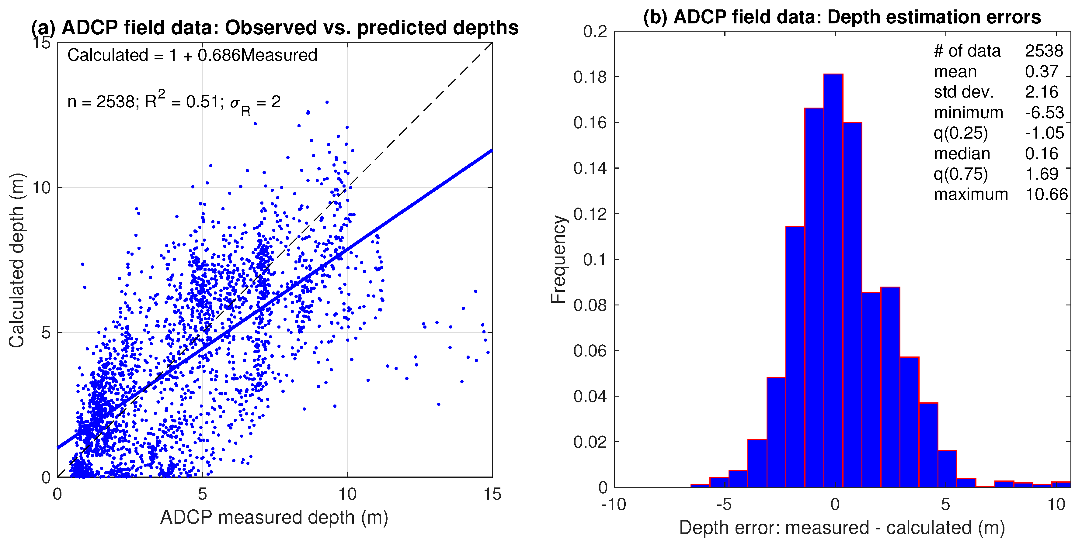
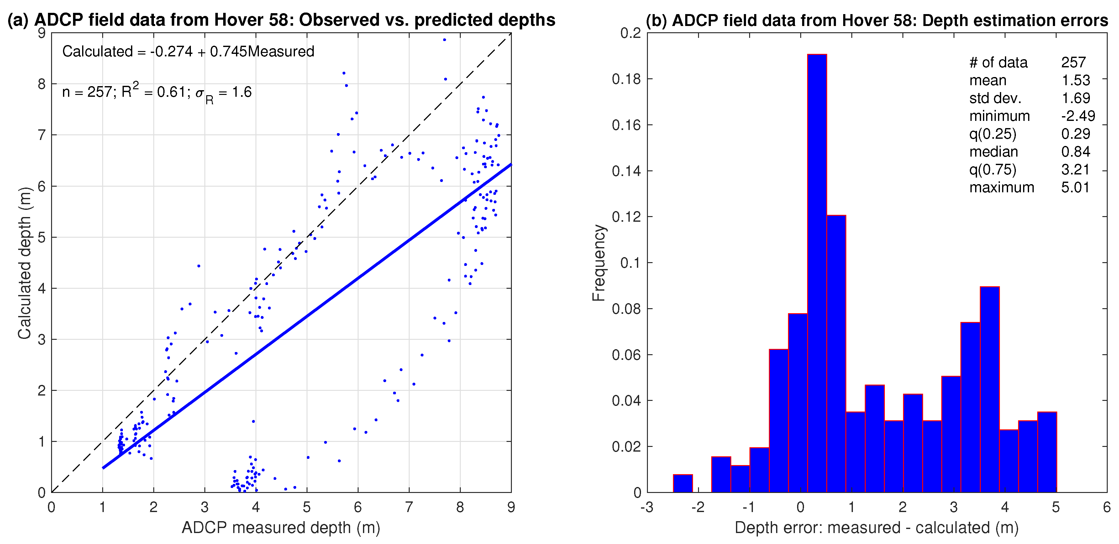
• Application of the DIVERS framework to field data resulted in modest agreement between observed and predicted depths ($R^2$ = 0.51 for the entire reach and 0.61 for a single transect in a straight section of the channel) and many large underestimates of depth, implying that the inherent limitations of the approach might constrain the accuracy with which depths can be inferred from remotely sensed velocities.
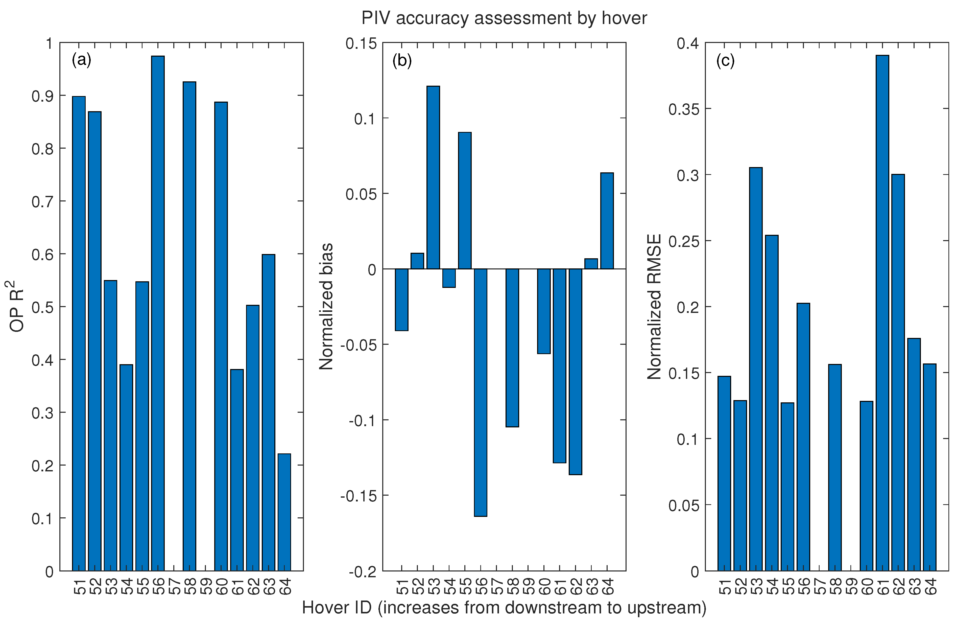
• Agreement between velocities measured directly in the field and estimated from remotely sensed data via PIV varied from hover to hover within the reach, with OP $R^2$ values ranging from 0.22 to 0.97 and a median value of 0.57. PIV-based velocities, which were not adjusted to convert surface velocities to depth-averaged velocities, did not consistently over-or under-predict the field observations. The median normalized mean bias was −2.7% and the median RMSE was 16.6%. These results suggest that velocities estimated by tracking naturally occurring sediment boil vortices were reasonably accurate and precise.
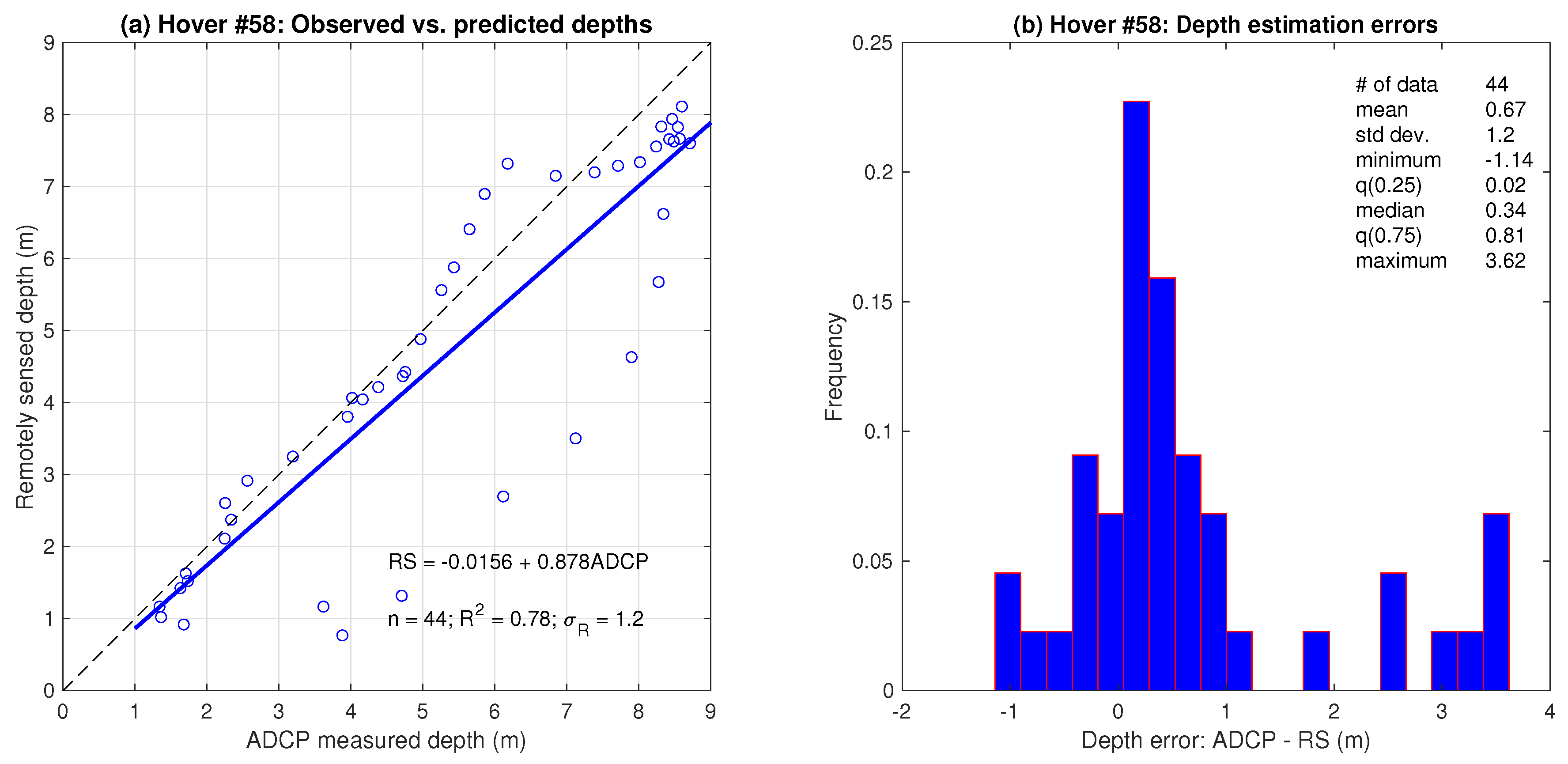
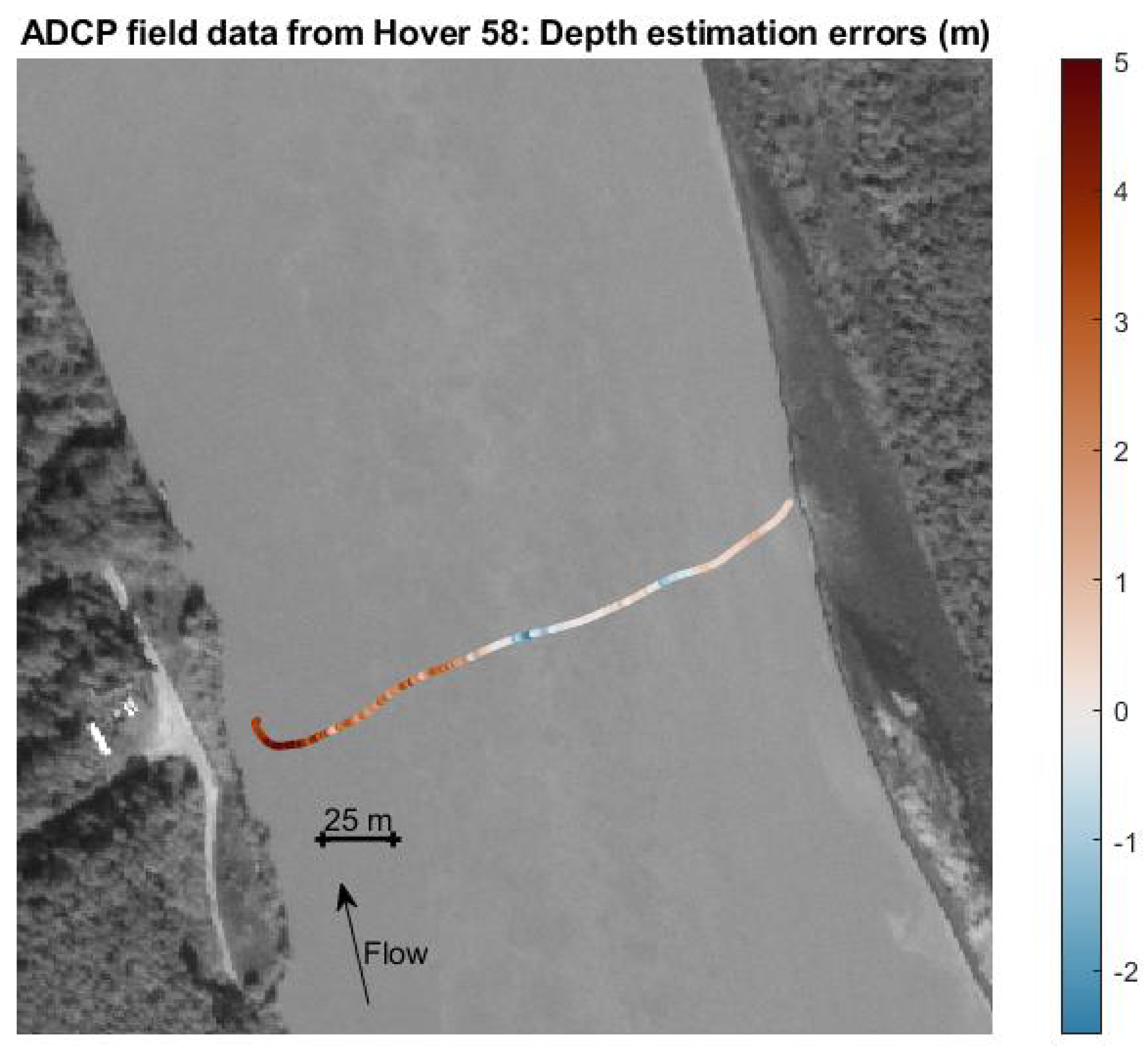
• For a single hover in a straight section, agreement between depths inferred via DIVERS and field measurements was stronger (OP $R^2$ of 0.78), with a smaller mean and standard deviation of errors than when DIVERS was applied to field data. Plotting a cross section illustrated the direct proportionality between PIV-derived velocities and depths calculated via DIVERS.
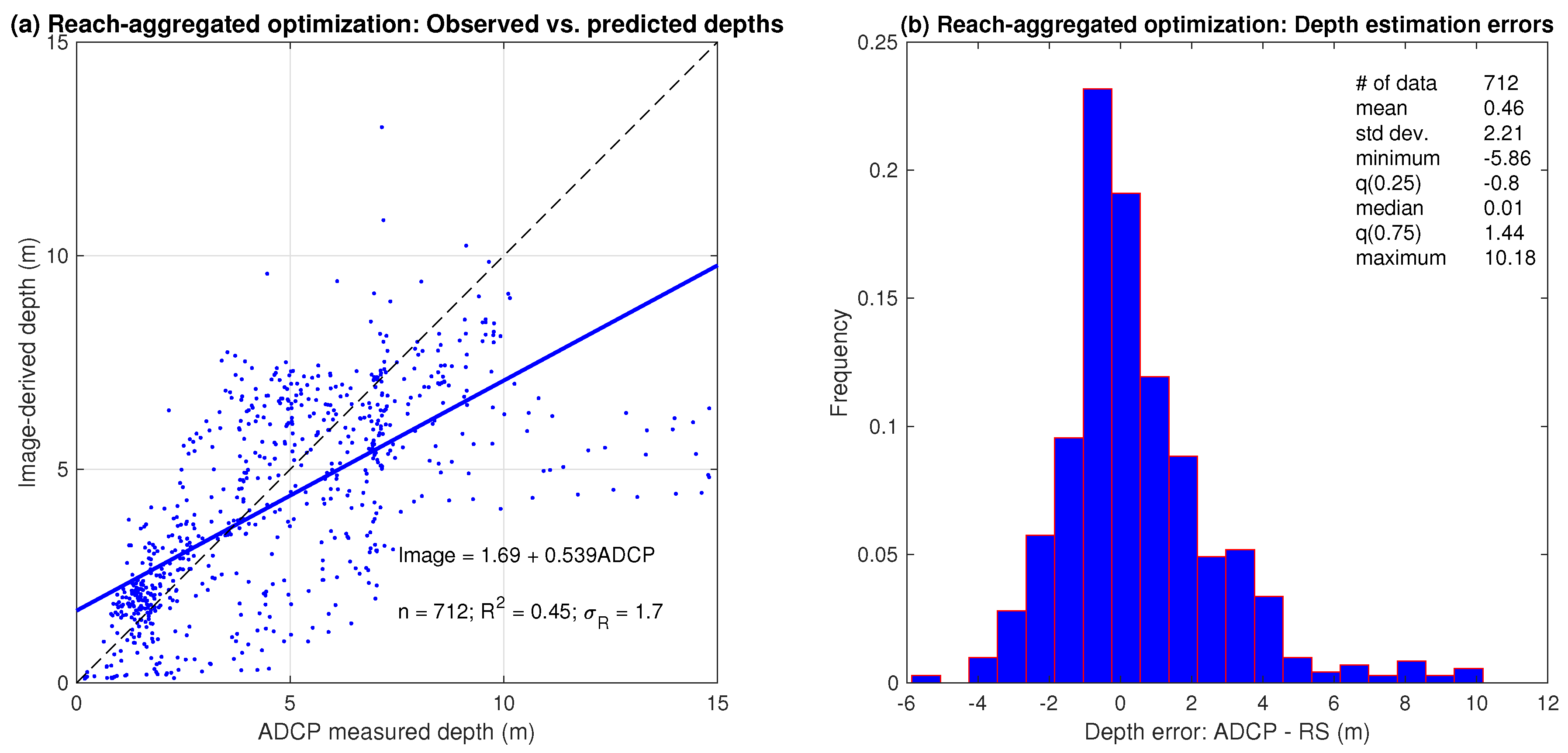
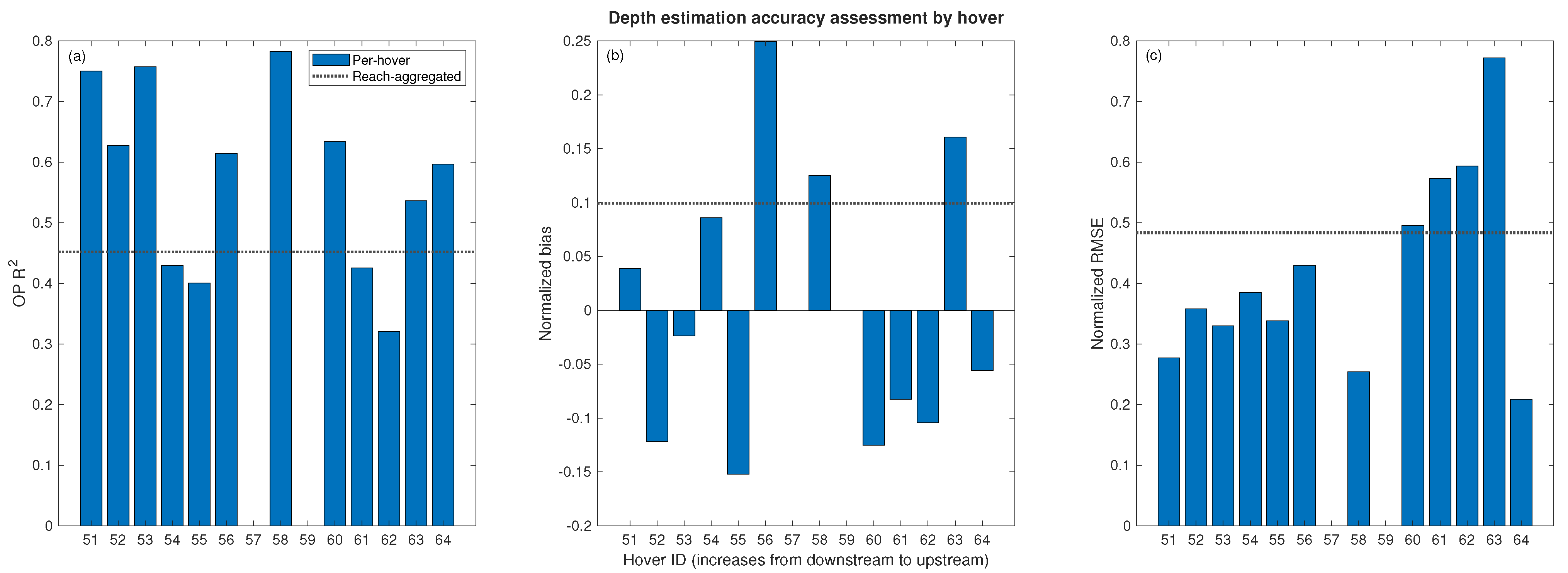
• Depth estimates were more accurate for a per-hover flow resistance optimization (FRO) approach (median normalized median bias of −4%) than for reach-aggregated FRO (10%). The precision of the two DIVERS variants was quantified in terms of the normalized RMSE, with values of 37% and 48% for the per-hover and reach-aggregated FRO methods, respectively.
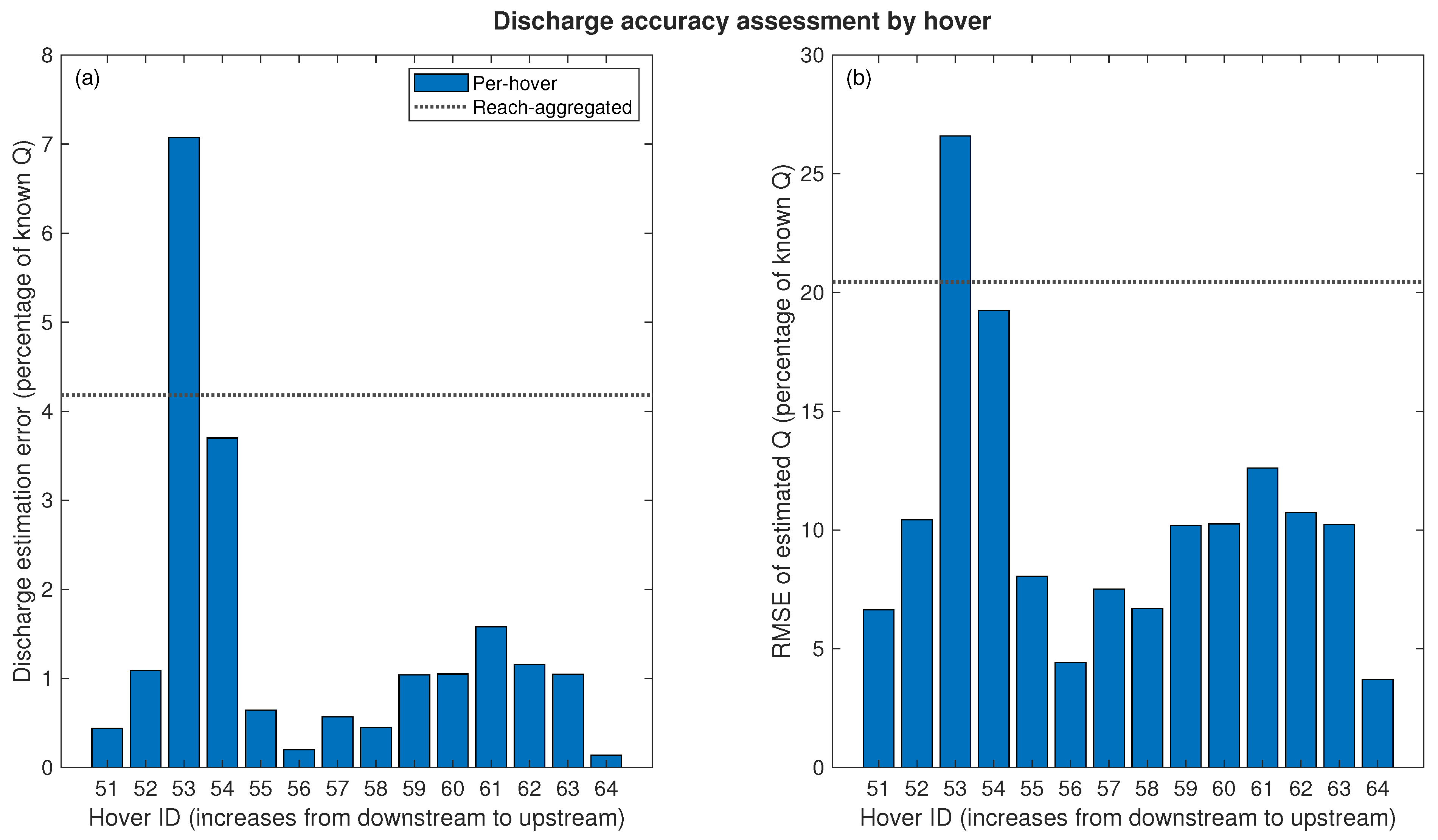
• The FRO algorithm successfully reproduced the discharge recorded at a gaging station to within a median of 1% on a per-hover basis and within 4% when cross sections were aggregated over the entire reach. The median normalized RMSE values for the discharge estimates from these approaches were 10% for per-hover FRO and 20% for reach-aggregated FRO.
• Although the assumptions inherent to the DIVERS framework impose some important limitations, this study demonstrated the potential of this approach to provide plausible, first-order approximations of water depth throughout the reach. These estimates could be refined through further research focused on incorporating more sophisticated numerical modeling techniques that account for processes, such as lateral transfer of momentum in meander bends, that are not represented in the initial iteration of DIVERS.

References

1. Conaway, J.; Eggleston, J.; Legleiter, C.; Jones, J.; Kinzel, P.; Fulton, J. Remote sensing of river flow in Alaska—New technology to improve safety and expand coverage of USGS streamgaging. U. S. Geol. Surv. Fact Sheet 2019, 2019, 4. [Google Scholar] [CrossRef] [Green Version]
2. Bjerklie, D.M.; Birkett, C.M.; Jones, J.W.; Carabajal, C.; Rover, J.A.; Fulton, J.W.; Garambois, P.A. Satellite remote sensing estimation of river discharge: Application to the Yukon River Alaska. J. Hydrol. 2018, 561, 1000–1018. [Google Scholar] [CrossRef] [Green Version]
3. Altenau, E.H.; Pavelsky, T.M.; Moller, D.; Pitcher, L.H.; Bates, P.D.; Durand, M.T.; Smith, L.C. Temporal variations in river water surface elevation and slope captured by AirSWOT. Remote Sens. Environ. 2019, 224, 304–316. [Google Scholar] [CrossRef] [Green Version]
4. Gleason, C.J.; Durand, M.T. Remote Sensing of River Discharge: A Review and a Framing for the Discipline. Remote Sens. 2020, 12, 1107. [Google Scholar] [CrossRef] [Green Version]
5. Legleiter, C.J.; Kinzel, P.J.; Nelson, J.M. Remote measurement of river discharge using thermal particle image velocimetry (PIV) and various sources of bathymetric information. J. Hydrol. 2017, 554, 490–506. [Google Scholar] [CrossRef]
6. Fulton, J.W.; Mason, C.A.; Eggleston, J.R.; Nicotra, M.J.; Chiu, C.L.; Henneberg, M.F.; Best, H.R.; Cederberg, J.R.; Holnbeck, S.R.; Lotspeich, R.R.; et al. Near-Field Remote Sensing of Surface Velocity and River Discharge Using Radars and the Probability Concept at 10 U.S. Geological Survey Streamgages. Remote Sens. 2020, 12, 1296. [Google Scholar] [CrossRef] [Green Version]
7. Kinzel, P.; Legleiter, C. sUAS-Based Remote Sensing of River Discharge Using Thermal Particle Image Velocimetry and Bathymetric Lidar. Remote Sens. 2019, 11, 2317. [Google Scholar] [CrossRef] [Green Version]
8. Fulton, J.W.; Anderson, I.E.; Chiu, C.L.; Sommer, W.; Adams, J.D.; Moramarco, T.; Bjerklie, D.M.; Fulford, J.M.; Sloan, J.L.; Best, H.R.; et al. QCam: sUAS-Based Doppler Radar for Measuring River Discharge. Remote Sens. 2020, 12, 3317. [Google Scholar] [CrossRef]
9. Bandini, F.; Sunding, T.P.; Linde, J.; Smith, O.; Jensen, I.K.; Köppl, C.J.; Butts, M.; Bauer-Gottwein, P. Unmanned Aerial System (UAS) observations of water surface elevation in a small stream: Comparison of radar altimetry, LIDAR and photogrammetry techniques. Remote Sens. Environ. 2020, 237, 111487. [Google Scholar] [CrossRef]
10. Legleiter, C.; Kinzel, P.J. Inferring Surface Flow Velocities in Sediment-Laden Alaskan Rivers from Optical Image Sequences Acquired from a Helicopter. Remote Sens. 2020, 12, 1282. [Google Scholar] [CrossRef] [Green Version]
11. Dugan, J.P.; Anderson, S.P.; Piotrowski, C.C.; Zuckerman, S.B. Airborne Infrared Remote Sensing of Riverine Currents. IEEE Trans. Geosci. Remote Sens. 2014, 52, 3895–3907. [Google Scholar] [CrossRef]
12. Muste, M.; Fujita, I.; Hauet, A. Large-scale particle image velocimetry for measurements in riverine environments. Water Resour. Res. 2008, 44, W00D19. [Google Scholar] [CrossRef] [Green Version]
13. Tauro, F.; Porfiri, M.; Grimaldi, S. Surface flow measurements from drones. J. Hydrol. 2016, 540, 240–245. [Google Scholar] [CrossRef] [Green Version]
14. Pearce, S.; Ljubičić, R.; Peña-Haro, S.; Perks, M.; Tauro, F.; Pizarro, A.; Dal Sasso, S.; Strelnikova, D.; Grimaldi, S.; Maddock, I.; et al. An Evaluation of Image Velocimetry Techniques under Low Flow Conditions and High Seeding Densities Using Unmanned Aerial Systems. Remote Sens. 2020, 12, 232. [Google Scholar] [CrossRef] [Green Version]
15. Strelnikova, D.; Paulus, G.; Käfer, S.; Anders, K.H.; Mayr, P.; Mader, H.; Scherling, U.; Schneeberger, R. Drone-Based Optical Measurements of Heterogeneous Surface Velocity Fields around Fish Passages at Hydropower Dams. Remote Sens. 2020, 12, 384. [Google Scholar] [CrossRef] [Green Version]
16. Eltner, A.; Sardemann, H.; Grundmann, J. Technical Note: Flow velocity and discharge measurement in rivers using terrestrial and unmanned-aerial-vehicle imagery. Hydrol. Earth Syst. Sci. 2020, 24, 1429–1445. [Google Scholar] [CrossRef] [Green Version]
17. Tosi, F.; Rocca, M.; Aleotti, F.; Poggi, M.; Mattoccia, S.; Tauro, F.; Toth, E.; Grimaldi, S. Enabling Image-Based Streamflow Monitoring at the Edge. Remote Sens. 2020, 12, 2047. [Google Scholar] [CrossRef]
18. Perks, M.T. KLT-IV v1.0: Image velocimetry software for use with fixed and mobile platforms. Geosci. Model Dev. Discuss. 2020, 13, 6111–6130. [Google Scholar] [CrossRef]
19. Lin, D.; Grundmann, J.; Eltner, A. Evaluating Image Tracking Approaches for Surface Velocimetry With Thermal Tracers. Water Resour. Res. 2019, 55, 3122–3136. [Google Scholar] [CrossRef]
20. Legleiter, C.; Harrison, L.R. Remote Sensing of River Bathymetry: Evaluating a Range of Sensors, Platforms, and Algorithms on the Upper Sacramento River, California, USA. Water Resour. Res. 2019, 55, 2142–2169. [Google Scholar] [CrossRef]
21. Bandini, F.; Lüthi, B.; Peña-Haro, S.; Borst, C.; Liu, J.; Karagkiolidou, S.; Hu, X.; Lemaire, G.G.; Bjerg, P.L.; Bauer-Gottwein, P. A Drone-Borne Method to Jointly Estimate Discharge and Manning’s Roughness of Natural Streams. Water Resour. Res. 2021, 57, e2020WR028266. [Google Scholar] [CrossRef]
22. Legleiter, C.; Kinzel, P. Helicopter-based videos and field measurements of flow depth and velocity from the Tanana River, Alaska, acquired on 24 Jul 2019. U. S. Geol. Surv. Data Release 2021, 12, 1282. [Google Scholar] [CrossRef]
23. USGS National Water Information System: USGS 15515500 TANANA R AT NENANA AK. Available online: https://waterdata.usgs.gov/nwis/inventory/?site_no=15515500 (accessed on 11 May 2021).
24. Wada, T.; Chikita, K.A.; Kim, Y.; Kudo, I. Glacial Effects on Discharge and Sediment Load in the Subarctic Tanana River Basin, Alaska. Arctic Antarct. Alp. Res. 2011, 43, 632–648. [Google Scholar] [CrossRef] [Green Version]
25. Chickadel, C.C.; Horner-Devine, A.R.; Talke, S.A.; Jessup, A.T.C.L. Vertical boil propagation from a submerged estuarine sill. Geophys. Res. Lett. 2009, 36, L10601. [Google Scholar] [CrossRef] [Green Version]
26. Talke, S.A.; Horner-Devine, A.R.; Chickadel, C.C.; Jessup, A.T. Turbulent kinetic energy and coherent structures in a tidal river. J. Geophys. Res. Ocean. 2013, 118, 6965–6981. [Google Scholar] [CrossRef] [Green Version]
27. Fujita, I.; Komura, S. Application of Video Image Analysis for Measurements of River-Surface Flows. Proc. Hydraul. Eng. JSCE 1994, 38, 733–738. [Google Scholar] [CrossRef]
28. Fujita, I.; Hino, T. Unseeded and Seeded PIV Measurements of River Flows Videotaped from a Helicopter. J. Vis. 2003, 6, 245–252. [Google Scholar] [CrossRef]
29. DJI Zenmuse X5. Available online: https://www.dji.com/zenmuse-x5 (accessed on 13 April 2021).
30. Teledyne Marine RiverRay ADCP. Available online: http://www.teledynemarine.com/riverray-adcp?ProductLineID=13 (accessed on 13 April 2021).
31. Hemisphere GNSS A101 Smart Antenna User Guide. Available online: https://www.hemispheregnss.com/wp-content/uploads/2019/01/hemispheregnss_a101_userguide_875-0324-000_b1.pdf (accessed on 13 April 2021).
32. Parsons, D.R.; Jackson, P.R.; Czuba, J.A.; Engel, F.L.; Rhoads, B.L.; Oberg, K.A.; Best, J.L.; Mueller, D.S.; Johnson, K.K.; Riley, J.D. Velocity Mapping Toolbox (VMT): A processing and visualization suite for moving-vessel ADCP measurements. Earth Surf. Process. Landforms 2013, 38, 1244–1260. [Google Scholar] [CrossRef]
33. Mueller, D.S. extrap: Software to assist the selection of extrapolation methods for moving-boat ADCP streamflow measurements. Comput. Geosci. 2013, 54, 211–218. [Google Scholar] [CrossRef]
34. Legleiter, C.J.; Kinzel, P.J. Surface Flow Velocities From Space: Particle Image Velocimetry of Satellite Video of a Large, Sediment-Laden River. Front. Water 2021, 3, 652213. [Google Scholar] [CrossRef]
35. Mueller, D.S. QRev—Software for Computation and Quality Assurance of Acoustic Doppler Current Profiler Moving-Boat Streamflow Measurements—User’s Manual for Version 2.8. In U. S. Geological Survey Open-File Report 2016-1052; US Department of the Interior, US Geological Survey: Reston, VA, USA, 2016. [Google Scholar] [CrossRef] [Green Version]
36. Mueller, D.S. QRev—Software for Computation and Quality Assurance of Acoustic Doppler Current profiler Moving-Boat Streamflow Measurements—Technical Manual for Version 2.8. In U. S. Geological Survey Open-File Report 2016-1068; US Department of the Interior, US Geological Survey: Reston, VA, USA, 2016. [Google Scholar] [CrossRef]
37. Cardona, A.; Saalfeld, S.; Schindelin, J.; Arganda-Carreras, I.; Preibisch, S.; Longair, M.; Tomancak, P.; Hartenstein, V.; Douglas, R.J. TrakEM2 Software for Neural Circuit Reconstruction. PLoS ONE 2012, 7, e38011. [Google Scholar] [CrossRef] [PubMed] [Green Version]
38. FIJI-ImageJ. Available online: https://imagej.net/Fiji (accessed on 14 April 2021).
39. Thielicke, W.; Stamhuis, E.J. PIVlab—Towards User-friendly, Affordable and Accurate Digital Particle Image Velocimetry in MATLAB. J. Open Res. Softw. 2014, 2, e30. [Google Scholar] [CrossRef] [Green Version]
40. Thielicke, W.; Stamhuis, E.J. PIVlab-Time-Resolved Digital Particle Image Velocimetry Tool for MATLAB. Figshare Dataset 2019, 12, 1092508.v19. [Google Scholar]
41. Nelson, J.M.; Bennett, S.J.; Wiele, S.M. Flow and sediment transport modeling. In Tools in Fluvial Geomorphology; Kondolf, G.M., Piegay, H., Eds.; Wiley: New York, NY, USA, 2003; pp. 539–576. [Google Scholar]
42. Smart, G.M.; Biggs, H.J. Remote gauging of open channel flow: Estimation of depth averaged velocity from surface velocity and turbulence. Proc. River Flow 2020, 2020, 1–10. [Google Scholar]
43. Le Coz, J.; Hauet, A.; Pierrefeu, G.; Dramais, G.; Camenen, B. Performance of image-based velocimetry (LSPIV) applied to flash-flood discharge measurements in Mediterranean rivers. J. Hydrol. 2010, 394, 42–52. [Google Scholar] [CrossRef] [Green Version]
44. Kinzel, P.J.; Legleiter, C.J.; Nelson, J.M.; Conaway, J.S.; LeWinter, A.L.; Gadomski, P.J.; Filiano, D. Near-field remote sensing of Alaska Rivers. In Proceedings of the 2019 Federal Interagency Sedimentation and Hydrologic Modeling Conference (SEDHYD), Reno, NV, USA, 24–28 June 2019. [Google Scholar]
45. Ferguson, R. Flow resistance equations for gravel- and boulder-bed streams. Water Resour. Res. 2007, 43, W05427. [Google Scholar] [CrossRef] [Green Version]
46. Legleiter, C. Calibrating remotely sensed river bathymetry in the absence of field measurements: Flow REsistance Equation-Based Imaging of River Depths (FREEBIRD). Water Resour. Res. 2015, 51, 2865–2884. [Google Scholar] [CrossRef]
47. Lagarias, J.C.; Reeds, J.A.; Wright, M.H.; Wright, P.E. Convergence Properties of the Nelder–Mead Simplex Method in Low Dimensions. SIAM J. Optim. 1998, 9, 112–147. [Google Scholar] [CrossRef] [Green Version]
48. Pineiro, G.; Perelman, S.; Guerschman, J.P.; Paruelo, J.M. How to evaluate models: Observed vs. predicted or predicted vs. observed? Ecol. Model. 2008, 216, 316–322. [Google Scholar] [CrossRef]
49. Global Mapper-All-in-one GIS Software. 2020. Available online: https://www.bluemarblegeo.com/products/global-mapper.php (accessed on 15 April 2021).
50. Toniolo, H. Bed Forms and Sediment Characteristics along the Thalweg on the Tanana River near Nenana, Alaska, USA. Nat. Resour. 2013, 4, 20–30. [Google Scholar] [CrossRef] [Green Version]
51. van Rijn, L.C. Sediment Transport, Part III: Bed forms and Alluvial Roughness. J. Hydraul. Eng. 1984, 110, 1733–1754. [Google Scholar] [CrossRef]
Figure 1. (a) Location of the study area along the Tanana River within the state of Alaska. The spatial footprints of the videos acquired while hovering above the channel are overlain on a background satellite image and ADCP field measurements of (b) depth-averaged flow velocity and (c) flow depth collected with an ADCP. Flow direction is from east to west (i.e., lower right to upper left). The red lines and corresponding numbers in (b,c) indicate helicopter hover ID numbers.
Remotesensing 13 04566 g001
Figure 2. Conceptual diagram outlining the data, user inputs, processing steps, and outputs of the DIVERS workflow for inferring water depths from remotely sensed surface flow velocities.
Remotesensing 13 04566 g002
Figure 3. Accuracy assessment of depths estimated from ADCP measurements of depth-averaged flow velocity for the entire reach: (a) Observed (measured in the field with an ADCP) vs. predicted (estimated from ADCP measurements of depth-averaged velocity using a flow resistance equation) regression output. (b) Distribution of depth estimation errors, defined as ADCP measurements minus estimates from flow resistance equation.
Remotesensing 13 04566 g003
Figure 4. Accuracy assessment of depths estimated from ADCP measurements of depth-averaged flow velocity for a single cross section located within Hover 58: (a) Observed (measured in the field with an ADCP) vs. predicted (estimated from ADCP measurements of depth-averaged velocity using a flow resistance equation) regression output. (b) Distribution of depth estimation errors, defined as ADCP measurements minus estimates from flow resistance equation.
Remotesensing 13 04566 g004
Figure 5. Accuracy assessment of particle image velocimetry (PIV)-derived surface flow velocity estimates by hover. Metrics of performance include (a) observed (measured in the field with an ADCP) vs. predicted (inferred from PIV) regression R 2 ; (b) Normalized bias of velocity estimation errors, with errors defined as ADCP-measured minus remotely sensed; and (c) normalized root mean square error (RMSE) of velocity estimation errors. Bias and RMSE are normalized by the reach-averaged mean of the velocity measurements used for accuracy assessment.
Remotesensing 13 04566 g005
Figure 6. Example output from Hover 58: (a) PIV-derived surface flow velocities extracted along 10 regularly spaced, channel-spanning cross sections. (b) Depths inferred by optimizing the flow resistance coefficient k to match the known discharge. (c) Surface velocities and depths extracted along an example cross section (#5 in (a)).
Remotesensing 13 04566 g006
Figure 7. Accuracy assessment of remotely sensed depths for Hover 58: (a) Observed (measured in the field with an ADCP) vs. predicted (inferred from PIV-derived surface flow velocities) regression output. (b) Distribution of depth estimation errors, defined as ADCP-measured minus remotely sensed.
Remotesensing 13 04566 g007
Figure 8. Sensitivity analysis to the flow resistance coefficient k for Hover 58. The following metrics are plotted as a function of k over the range from half to twice the k value identified as optimal, which is indicated by the dashed vertical line in each panel: (a) discharge estimation error, expressed as a percentage of the known discharge, with errors defined as the known discharge minus that estimated via remote sensing; (b) root mean square error (RMSE) of discharge estimates, expressed as a percentage of the known discharge; (c) normalized bias of depth estimation errors, with errors defined as ADCP-measured minus remotely sensed; and (d) normalized root mean square error (RMSE) of depth estimation errors. Bias and RMSE are normalized by the mean of the depth measurements used for accuracy assessment.
Remotesensing 13 04566 g008
Figure 9. Sensitivity analysis to water surface slope S for Hover 58. The following metrics are plotted as a function of S over the range from half to twice the S value measured from the lidar DEM (0.00014), which is indicated by the dashed vertical line in each panel: (a) discharge estimation error, expressed as a percentage of the known discharge, with errors defined as the known discharge minus that estimated via remote sensing; (b) root mean square error (RMSE) of discharge estimates, expressed as a percentage of the known discharge; (c) normalized bias of depth estimation errors, with errors defined as ADCP-measured minus remotely sensed; and (d) normalized root mean square error (RMSE) of depth estimation errors. Bias and RMSE are normalized by the mean of the depth measurements used for accuracy assessment.
Remotesensing 13 04566 g009
Figure 10. Estimated discharges for cross sections aggregated over the 14 hovers to span the entire reach. The locations of the midpoints of each transect of ADCP field data are represented by the red X symbols at the bottom of the plot. The known discharge measured at the gaging station is indicated by the dashed horizontal line and the dashed vertical lines bracket the cross sections included within each of the hovers.
Remotesensing 13 04566 g010
Figure 11. Accuracy assessment of remotely sensed depths for cross sections aggregated over the entire reach. (a) Observed (measured in the field with an ADCP) vs. predicted (inferred from PIV-derived surface flow velocities) regression output. (b) Distribution of depth estimation errors, defined as ADCP-measured minus remotely sensed.
Remotesensing 13 04566 g011
Figure 12. Accuracy assessment of depth estimates by hover for the per-hover optimization approach, indicated by blue bars. The results for the reach-aggregated optimization approach also are included and are represented by the dashed horizontal line because a single value pertains to the entire reach (i.e., all of the hovers). Metrics of performance include (a) observed (measured in the field with an ADCP) vs. predicted (inferred from PIV) regression R 2 ; (b) normalized bias of depth estimation errors, with errors defined as ADCP-measured minus remotely sensed; and (c) normalized root mean square error (RMSE) of depth estimation errors. Bias and RMSE are normalized by the reach-averaged mean of the depth measurements used for accuracy assessment.
Remotesensing 13 04566 g012
Figure 13. Accuracy assessment of discharge estimates by hover for the per-hover optimization approach, indicated by blue bars. The results for the reach-aggregated optimization approach also are included and are represented by the dashed horizontal line because a single value pertains to the entire reach (i.e., all of the hovers). Metrics of performance include (a) discharge estimation error, expressed as a percentage of the known discharge, with errors defined as the known discharge minus that estimated via remote sensing; (b) root mean square error (RMSE) of discharge estimates, expressed as a percentage of the known discharge.
Remotesensing 13 04566 g013
Figure 14. Accuracy assessment of depths estimated from ADCP measurements of depth-averaged flow velocity for a single cross section located within Hover 58: Map of depth estimation errors, defined as ADCP measurements minus estimates from flow resistance equation.
Remotesensing 13 04566 g014
Figure 15. Depth map mosaics derived from cross sections (a) aggregated over the entire reach and (b) individual hovers.
Remotesensing 13 04566 g015