Abstract
Prediction of soft soil settlement is an important research topic in the field of civil engineering, and the least square support vector machine is one of the commonly used prediction methods at present. Nonetheless, the existing LSSVM models have problems of low search efficiency in the search process and lack of global optimal solution in the search results. In order to solve this problem, based on the leave-one-out cross-validation method, the homotopy continuation method was used to optimize the LSSVM model parameters, and then the HC-LSSVM model was constructed with the goal of minimizing the sum of squares of the prediction error of the full sample retention one. Finally, the rationality and correctness of the model are verified by engineering application. The results show that the HC-LSSVM model constructed in this study can accurately predict the settlement of soft ground, which is superior to the common LSSVM model and solves the problem that the parameters of LSSVM model cannot be solved optimally. The research results provide a new method for prediction of soft soil settlement.
1. Introduction
More and more buildings, roads and railways are built on soft soil, and their construction schemes and use functions require more accurate determination of their settlement in the construction period and operation period [1]. Now there are effective stabilization technologies to reduce settlement, such as the realization of pile foundations [2,3]. However, the settlement prediction of soft soil is still an important topic in civil engineering research to effectively prevent disasters [4,5,6]. Common soft soil settlement prediction methods include curve-fitting method and system theory method, among which curve-fitting method includes hyperbola method, exponential curve method, three-point method, Asaoka method, settlement rate method, Xinye method, etc. [7], and the system theory method includes grey theory method, neural network method, Support Vector Machines (SVM), and its improvement method [8,9,10,11]. Least Squares Support Vector Machines (LSSVM) is one of the improvement methods of SVM, which changes the problem of solving quadratic programming in the optimization problem of SVM into the problem of solving linear equations. Similar to SVM methods, they are based on statistical learning theory and adopt the principle of minimum structural risk to maximize their generalization ability and better solve practical problems such as nonlinearity, high dimension and local minimum. The difference is that LSSVM method simplifies the model solving difficulty and improves the model calculation speed compared with SVM method [12]. However, the current LSSVM method still has the deficiency of less guidance in the search process or the optimized parameters are not the global optimal solution when solving the model parameters. Therefore, it is necessary to conduct in-depth research on the LSSVM method to be more suitable for the prediction of soft ground settlement.
In terms of settlement prediction, the LSSVM method is the same as the SVM method, and the selection of hyperparameters has a great influence on the solution accuracy of the prediction problem. Therefore, the choice of what kind of effective method to establish the hyperparameters of the model becomes a key problem of SVM model or LSSVM model. Research on this problem can be summarized into two categories: one is intelligent method and optimization method of parameter selection. For example, Mohanty et al. combine non-dominated sorting genetic algorithm (NSGA II) with a learning algorithm (neural network) to establish a prediction model based on SPT data based on Pareto optimal frontier [13]. Li et al. introduced MAE, MAPE, and MSE as the criteria to evaluate the prediction accuracy of SP-LSSVM and MP-LSSVM, and then optimized LSSVM hyperparameters [14]. Similarly, Zhang et al. proposed MAE and RMSE optimization model parameters, and explained the correspondence between WPT-LSSVM model prediction and actual observation [15]. Kumar et al. used 18 statistical parameters, such as RMSE and T-STAT to optimize LSSVM model parameters, and compared the reliability of LSSVM, GMDH and GPR models [16]. Another method is to optimize parameters by using the physical characteristics of samples in the model, including the output error of samples, the algebraic distance of samples, the number of key samples, etc. For example, Samui et al. selected geotechnical parameters related to the geometric shape of shallow foundation as the input values of training samples, determined regularization parameters by analyzing the correlation coefficient of output values, and proved that this method has good usability through testing samples [17]. Kundu et al. used physical characteristics such as rainfall, minimum temperature, and maximum temperature at different elevations as input values of training samples, selected parameters related to output values, and used relevant physical quantities at another elevation as test samples to compare the overall performance of LSSVM model and SDSM model [18]. Chapelle et al. used a leave-one-out cross-validation method and support vector counting to optimize SVM parameters: the leave-one-out cross-validation method divided the sample set into a training sample set and a test sample set, and the minimum statistical index of test error rate of SVM for many times was used as the criterion of optimization parameters; the support vector counting method takes the minimum ratio of the number of support vectors to the total number of samples as the criterion of SVM parameter optimization [19]. Both methods have their advantages and disadvantages in solving model parameters: the first method solves parameters by intelligent method or optimization method, which can comprehensively search the optimal solution of model parameters. However, due to the lack of physical model guidance in the search process, the search efficiency is low. The second method uses the physical characteristics of the samples in the model to optimize parameters. In the process of parameter optimization, the model has more guidance and the search time is short, but due to the simplified physical characteristics, the optimized parameters are not the global optimal solution. Therefore, it is necessary to further improve the LSSVM model to solve the two problems of low search efficiency in the search process and lack of global optimal solution in the search results.
In general, in order to make full use of the advantages and overcome the disadvantages of the two methods of LSSVM model parameter solving, this study proposes the HC-LSSVM model: based on the leave-one-out cross-validation method, the optimization problem of LSSVM model parameters is transformed into the solution problem of nonlinear equations with the goal of minimizing the sum of squares of the prediction error of full sample retention one, and considering that the homotopy continuation method is an effective method to solve nonlinear equations in a large range of search [20,21], the homotopy continuation method is adopted to solve the nonlinear equations, and the results of solution are taken as the optimal parameters of LSSVM model. Finally, this study tested the model through the measured data of soft soil settlement, and the test results proved that the LSSVM model had a good optimization result and the LSSVM model is a stable model with a good prediction result in the selection of hyperparameters (Figure 1).
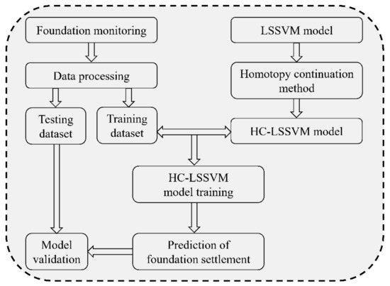
Figure 1.
Research ideas and steps.
2. Methods
2.1. LSSVM Model for Soft Ground Settlement Prediction
LSSVM is a method based on statistical learning theory. It is of great significance and good effect to apply LSSVM to the settlement prediction of soft soil, but the choice of model parameters has a great influence on the prediction accuracy. Therefore, on the basis of the fast retention one method, this study intends to minimize the sum of squares of the prediction error of the full sample retention one as the goal and transform the parameter optimization problem of the LSSVM model into the problem of solving nonlinear equations. Meanwhile, the homotopy continuation method is used to solve the nonlinear equations, and the solution results are used as the optimal parameters of the LSSVM model.
LSSVM uses the principle of function regression estimation to establish the model based on the monitoring value of soft soil settlement as the training set, and achieves the learning and prediction purpose by accurately monitoring and predicting the settlement of soft soil. Therefore, the training set of soft soil settlement samples must be established before LSSVM is used for learning and prediction. Suppose the training set, (x1, y1), …, (xi, yi), …, (xn, yn), where xi ∈ Rm, yi ∈ Rn, i = 1, 2, …, n; xi is the input vector, and in this study, is the cumulative settlement time of soft soil; yi is the output vector, and in this study, is the cumulative settlement amount of soft soil. The problem of functional regression estimation is to find a function f after learning the training set, so that yd = f(xd) corresponding to any test sample xd (cumulative settlement time of soft soil) outside the training set can be found, and the deviation between yd and its truth value y (cumulative settlement of soft soil) can be minimized. In its principle, LSSVM uses functions of the following form to perform regression estimation of unknown functions [18]:
where Φ: Rm→H, Φ is the feature mapping, H is the feature space, w is the weight vector in space H, and b ∈ Rn is the offset parameter.
LSSVM transforms the above regression estimation problem into risk minimization problem of loss function by introducing loss function. In this study, it is the problem of minimizing the error between the predicted value and the actual value of soft soil settlement, and adopts the structured risk minimization principle to conduct risk minimization analysis, and obtains the following optimization problems and constraints [16,17],
where C is adjustable regularization parameter and ek is error variable.
As it is difficult to solve Equation (2) directly, LSSVM adopts duality theory to solve and establish Lagrange equation and its optimization conditions [17],
where α is the Lagrange multiplier. If the absolute value of the Lagrange multiplier is very small, it makes very little contribution to the regression of the model, and its corresponding samples are called non-support vectors. In other cases, the samples corresponding to the Lagrange multiplier are called support vectors.
According to Mercer’s condition [14], there is a kernel function K(xk, xl):
Solve the optimization condition (Equation (5)), eliminate w, and ei, and replace ΦT(xk)Φ(xl) with K(xk,xl). Finally, the parameter optimization problem is transformed into the problem of solving a system of linear equations.
The LSSVM algorithm uses the least square method to solve the linear equations represented by Equation (7), avoiding the convex quadratic programming problem in the standard support vector machine algorithm, and has better prediction performance than the traditional support vector machine method.
LSSVM has the same principle as SVM. In order to conduct sample training and estimation, some model parameters must be defined first, such as those in Equation (4). Meanwhile, the prediction accuracy of LSSVM is greatly affected by the selection value of model parameters. Therefore, this study adopts the fast retention method proposed by Van Gestel et al. [22] to optimize LSSVM parameters.
Suppose
Then, Equation (7) can be expressed as
Then, S = A−1●Y is the LSSVM coefficient solution of the whole sample, and the leave-one-out cross-validation method is adopted for the training sample set, then the LSSVM coefficient solution of the p th time can be expressed as [22]
where S(p) is the p th element in S, S(p−) is the column vector of S after removing the p th element, A−1(p,p) is the element of the p th row and the p th column in A−1, and A−1(p−,p) is the column vector of the p th column in A−1 after removing the p th element.
It is assumed that the kernel function takes the radial basis function (RBF function) [12],
where σ2 is the kernel parameter, denoted as sig2. Note .
Meanwhile, as the LSSVM model parameters are (C,sig2), the error of the LSSVM model for the p th individual can be expressed as
where K′(p,p−) is the row vector of the p th row in the matrix K′ after removing the p th element.
Therefore, the leave-one-out error of the whole sample can be expressed as
In order to obtain the optimal parameters of LSSVM model, the key is to minimize sse(C,sig2) value represented by Equation (12). Therefore, the optimal parameters of LSSVM model should meet Equation (13),
In order to solve Equation (13), this study mainly constructs the homotopy equation of Equation (13) and uses the homotopy continuation method to solve Equation (13). The solutions obtained are used as the preferred parameters of LSSVM model.
2.2. LSSVM Model Parameter Solution Based on Homotopy Continuation Method
The HC-LSSVM model of soft soil settlement based on homotopy continuation method is mainly expressed as follows: based on the observation data of soft soil settlement, the training sample set and test sample set are established, and on the basis of leave-one-out cross-validation method, the optimization problem of LSSVM model parameters is transformed into solving nonlinear equations problem with the goal of minimizing the sum of squares of prediction error for the whole sample. The homotopy continuation method is used to solve nonlinear equations. The solution results were taken as the optimal parameters of LSSVM model, and the optimal parameters were used to predict the settlement of the test sample set. The construction method of HC-LSSVM model is described as follows.
- (1)
- Establish training sample set and test sample set based on soft soil settlement observation data.
- (2)
- Construct the homotopy equation:where C0 and sig20 are the initial LSSVM model parameters. When t = 1, the obtained solutions of are the optimal LSSVM model parameters.Suppose the known solution of is . In order to find the solution curve = of the homotopy equation, take the derivative of parameter t, then the solution problem of nonlinear equations is transformed into the initial value problem of differential equations,
- (3)
- The grid search method was used to select the LSSVM model parameters: the initial regularization parameter C0 and the kernel parameter sig20. The grid search range of LSSVM parameters was given and the corresponding grid search step was set. Set the grid search stop conditions, including stop the search when the maximum search times are met, stop the search when t = 1 is met when the first homotopy path is found, and stop the search when the LSSVM model parameters exceed the grid search range.
- (4)
- Set the initial value t = 0 of the homotopy parameter t, and set the homotopy parameter step t_step.
- (5)
- Set the iteration stop condition of the Euler forecaster-Newton correction method [23,24], and repeatedly use Euler forecaster-Newton correction method to solve Equation (15) until the iteration stop condition is satisfied.First, the next approximate point of the homotopy path is obtained by euler estimation method,Then, Newton’s correction method is used to correct the approximate points,In order to simplify the calculation of partial derivatives and , the following equation is adopted in this study to simplify the calculation of partial derivatives,where C_step and sig2_step are step sizes. Therefore, proper C_step and sig2_step must be selected before solving the equations with Euler estimation-Newton correction method. Iteration stop conditions include iteration stops when C < 0 and sig2 < 0; iteration stops when t = 1. Optimization parameters C′ and sig2′ were obtained after iteration.
- (6)
- If the first homotopy path ending condition t = 1 is not found, the initialization LSSVM model parameters and the grid search step are modified. If the homotopy path end condition is t = 1, then the LSSVM model parameters are the LSSVM model parameters optimized by homotopy continuation method.
- (7)
- The HC-LSSVM regression model was established by using the LSSVM model parameters optimized by homotopic continuation method, and the settlement of the test sample set was predicted, and the corresponding prediction results were finally output.
2.3. HC-LSSVM Model for Prediction of Soft Soil Settlement
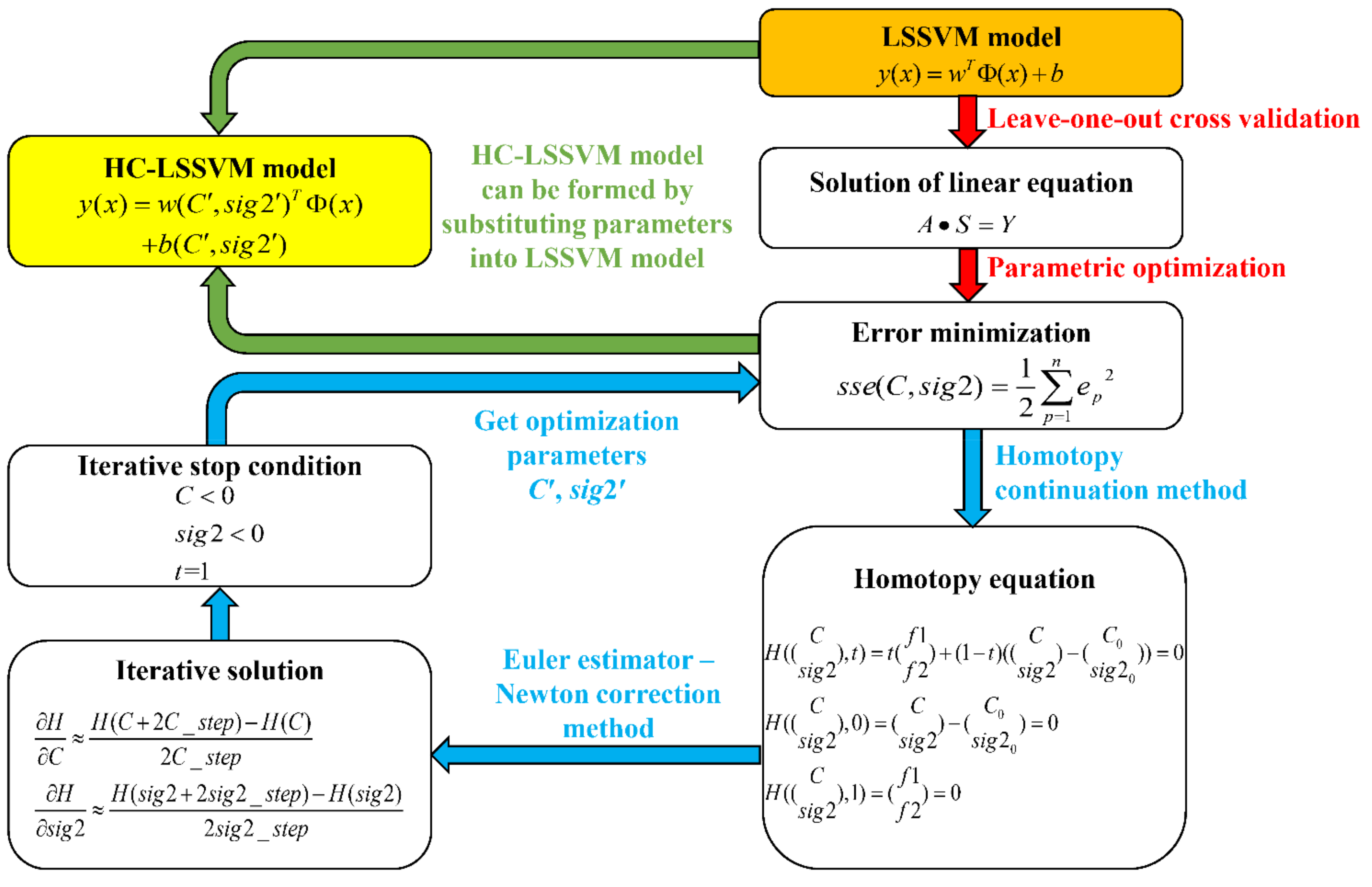
Based on the above analysis of the LSSVM model for soft soil settlement prediction and the solution of LSSVM model parameters based on homotopy continuation method, this study established the HC-LSSVM model for soft soil settlement prediction, and its construction process and solution method are shown in Figure 2. According to the traditional LSSVM model (Equation (1)), the linear equations (Equations (7) and (8)) were established to solve the parameters. Then, the homotopy equation (Equation (14)) was established according to the error minimization optimization conditions (Equations (12) and (13)) and the homotopy continuation method. The optimization parameters C′ and sig2′ were obtained through the iterative solution (Equation (18)) and substitute the parameters into the traditional LSSVM model again to obtain the HC-LSSVM model (Equation (19)).
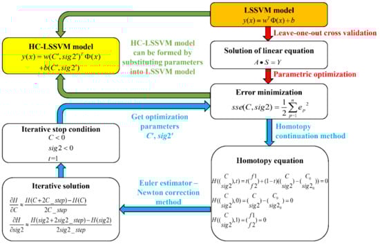
Figure 2.
Block diagram of HC-LSSVM model for soft soil settlement prediction. The orange box is the starting position of the block diagram, and the yellow box is the end position of the block diagram. The arrows in different colors represent the sequence of the model building process, with the red sorted as 1, the light blue sorted as 2, and the green sorted as 3.
3. Results and Discussion
3.1. Soft Soil Settlement
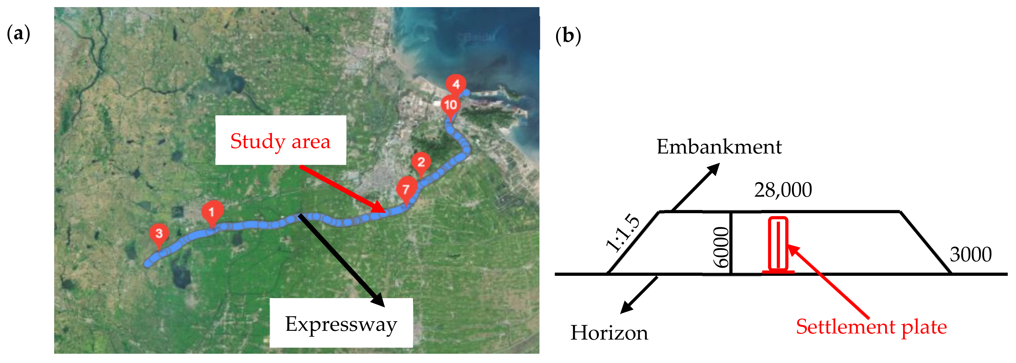
In order to test the reliability of the HC-LSSVM model proposed in this study, the cumulative settlement of the embankment center of an expressway in eastern China is selected as the research object. The locations of the expressway and the study area in this paper are shown in Figure 3a. With a total length of 237 km, the expressway undertakes the important task of transportation in the east and west of China. The whole line of the expressway is designed according to the standards of full closure, full interchange and two-way four-lane. The design speed is 120 km/h and the embankment width is 28 m. The expressway is divided into five sections A, B, C, D, and E according to administrative regions. The location of the data collected in this study is section A [25,26].

Figure 3.
Expressway location and schematic diagram of embankment settlement observation. (a) Location and study area of Expressway. (b) Schematic diagram of embankment cross-section and settlement monitoring (the unit of measurement is mm).
The embankment in the area of concern of this study is constructed of soft soil. The thickness of soft soil L in this area is 3.9–9.0 m, mainly composed of silt and clay according to the classification of the Code for Investigation of Geotechnical Engineering (GB 50021-2001 (2009)) [27], with a void ratio e of 1.2–2.1, a Poisson’s ratio n of 0.40–0.50, a natural moisture content wn of more than 50% and locally as high as 80%, a liquid limit wL of generally 40–60%, a consolidation coefficient Cv of 0.2 × 10⁻³–0.7 × 10⁻³ cm2/s, an over-consolidation ratio OCR < 1, a coefficient of permeability k of 1 × 10⁻⁴–1 × 10⁻⁸ cm/s, a compression index Cc of 0.8–0.9, the rebound index Cr of 0.09, the unconfined compressive strength qu of 25–50 kPa, a Young’s modulus of elasticity E of 2.0–5.0 MPa, and a groundwater level h of 1.0–2.0 m [26].
The embankment cross section and embankment settlement monitoring location of expressway are shown in Figure 3b. The embankment height is ~6000 mm (relative to horizontal plane), the embankment width is 28,000 mm, the berm width is 3000 mm, and the embankment slope is 1:1.5. Three embankment settlement monitoring points are set in the embankment center, and the settlement is measured by landmark method (settlement plate). The settlement plate is composed of steel bottom plate, reinforced concrete plate, metal measuring rod, and protective sleeve [25,28]. The following is the monitoring and calculating data of central settlement of soft soil embankment of the expressway (Table 1) [26]. The observation data with cumulative settlement time from 0 to 587 days are taken as training samples, and the observation data from 618 to 742 days are taken as test samples.

Table 1.
Monitoring data of soft soil settlement.
3.2. Training and Testing of the HC-LSSVM Model
According to the construction method of the HC-LSSVM model (Section 2.2) and the training samples of soft soil settlement, after many comparisons, the following HC-LSSVM model solution process and parameters are set. (1) Set the predicted embedding dimension to 2, that is, the dimension of the input vector Xi is 2. (2) The sample data must satisfy the nonlinear mapping relationship between the autocorrelation Xi = {xi − 1,xi − 2} and the output Yi = {xi}, where xi is the soft soil settlement time of a group of observed data. (3) The radial basis function (RBF function) was taken as the kernel function, the grid search range was set C ∈ [1, 2500] and sig2 ∈ [1, 1000], the initial regularization parameter C0 = 100 and the kernel parameter sig20 = 10, and the grid search step was C_step = 30 and sig2_step = 10. (4) Set the homotopy parameter step t_step = 0.2. After a multi-step grid search, the optimal LSSVM model parameters were obtained as C = 209 and sig2 = 24. The HC-LSSVM model was established based on the optimized LSSVM model parameters, and settlement prediction was carried out for the test samples.
According to the optimization parameters obtained by the above HC-LSSVM model, the comparison between the predicted value and the monitored actual value of the training samples is shown in Figure 4. The predicted value is very close to the actual value in Figure 4, and the average error εa is only 1.55%, which proves the reliability of the optimized parameters obtained by HC-LSSVM model.
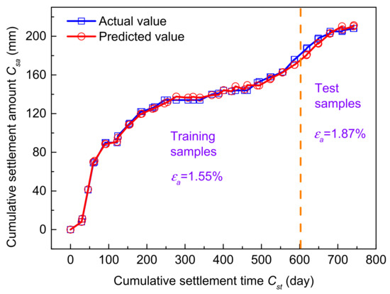
Figure 4.
Comparison between predicted and actual value of soft soil settlement of training samples and test samples.
The observation data from 618 days to 742 days were taken as the test samples, and the test results are shown in Table 2 and Figure 4. It can be seen from Table 2 that the trained HC-LSSVM model is very close to the cumulative settlement of the embankment center. The error ε between predicted and actual value of settlement amount (Pv and Av) is between 0.50% and 3.62%, and the average error εa is 1.87%. This shows that the prediction of soft soil settlement according to the optimized parameters obtained by HC-LSSVM model can get very close to the monitored actual value.
Table 2.
Comparison between predicted and actual value of soft soil settlement of test samples.
3.3. Evaluation of the HC-LSSVM Model
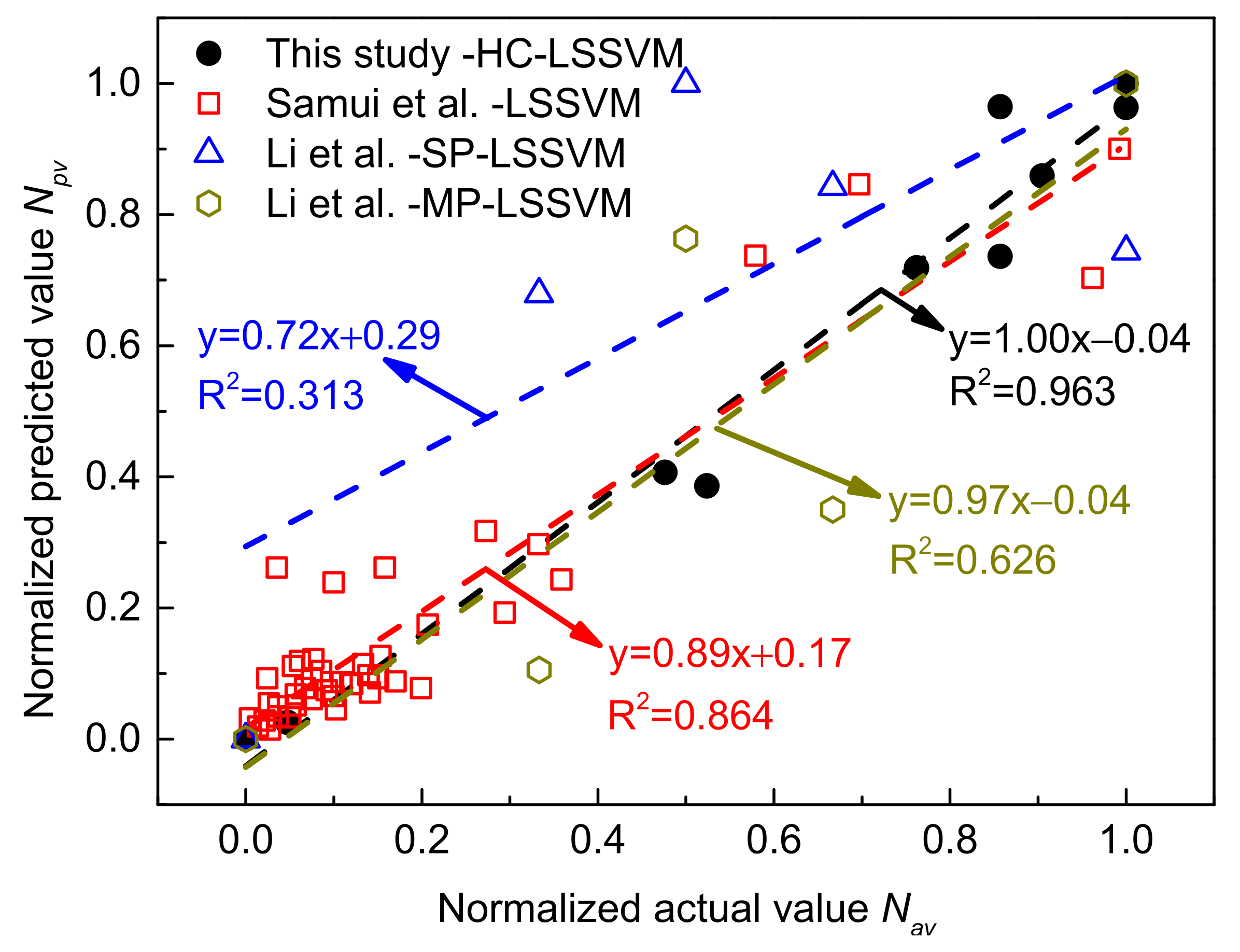
The settlement of soft soil has caused a large number of casualties and property losses. It is very important to monitor and predict the settlement of soft soil accurately for construction management. Displacement analysis and prediction is a key step in soft soil monitoring and early warning control. Previous basic prediction methods such as the LSSVM model have certain limitations in data processing prediction accuracy, so this study proposes HC-LSSVM model combined with homotopy continuation method. In order to evaluate the reliability of the HC-LSSVM model, the model was compared with previous research results [14,17] (Figure 5). For the convenience of comparison and analysis, both predicted and actual values in the research results are expressed in normalized form in Figure 5 (Equation (20)). The linear fitting of the research results shows that the slope of the line is 1.00 and the correlation coefficient R2 is as high as 0.963, which again verifies the reliability of the research results in this study. Other research results (Li et al. -MP-LSSVM) also have the slope of the fitting line of 0.97, which is very close to the optimal value of 1.00, but the correlation coefficient R2 is only 0.626, indicating that the data is extremely unstable. Of course, some research results (Samui et al. (LSSVM)) have very high correlation coefficient and good fitting effect, but the slope of the fitting line is only 0.89, which is far from the optimal value of 1.00. In conclusion, the HC-LSSVM model established in this study can better predict soft soil settlement, its development law is in good agreement with the actual situation, and the prediction effect is better than other LSSVM models. On the basis of acquiring more learning samples, the HC-LSSVM model in this study can also predict the settlement value of soft soil for a long time,
where Xn is the normalized predicted value or monitored value, Xr is the predicted value or monitored value before the normalization, Xmax is the maximum predicted value or monitored value before the normalization, and Xmin is the minimum predicted value or monitored value before the normalization.
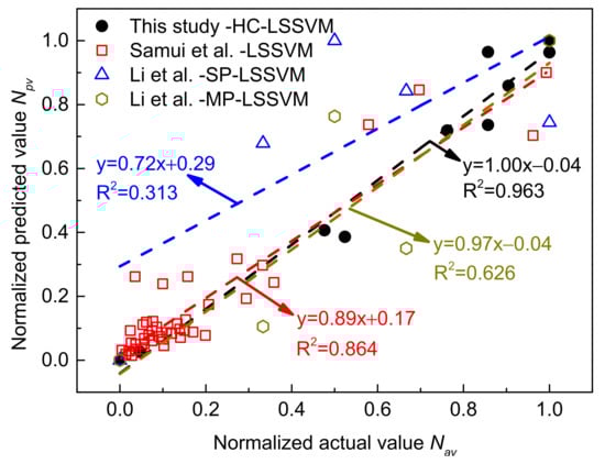
Figure 5.
Comparison between the HC-LSSVM model and other research results.
4. Conclusions
- (1)
- On the basis of the leave-one-out cross-validation method, the homotopy continuation method was used to optimize the LSSVM model parameters with the goal of minimizing the sum of squares of the prediction errors of the full sample retention one, and then the HC-LSSVM model was constructed, which solved the problems of low search efficiency in the search process and lack of global optimal solution in the search results of the existing LSSVM models.
- (2)
- Comparing with training samples and test samples, the HC-LSSVM model can accurately predict soft soil settlement, and the prediction result is significantly better than that of ordinary LSSVM model.
- (3)
- The research results provide a new method for the prediction of soft soil settlement. The prediction of future settlement amount based on the existing observation data can effectively prevent the occurrence of disasters.
Author Contributions
Conceptualization, C.Z. and Z.L.; methodology, Z.L.; software, G.C. and S.X.; validation, Z.L. and G.C.; formal analysis, Z.L. and G.C.; investigation, G.C. and S.X.; resources, C.Z. and Z.L.; data curation, G.C. and S.X.; writing—original draft preparation, G.C. and S.X.; writing—review and editing, G.C. and Z.L.; visualization, G.C. and Z.L.; supervision, G.C. and Z.L.; project administration, C.Z.; funding acquisition, C.Z. All authors have read and agreed to the published version of the manuscript.
Funding
This research was funded by the National Key Research and Development Project, Grant Number 2017YFC1501203 and 2017YFC1501201; the National Natural Science Foundation of China (NSFC), Grant Number 41977230; and the Special Fund Key Project of Applied Science and Technology Research and Development in Guangdong, Grant Number 2015B090925016 and 2016B010124007.
Institutional Review Board Statement
Not applicable.
Informed Consent Statement
Not applicable.
Data Availability Statement
The data presented in this study are available in the article.
Acknowledgments
The authors would like to thank the anonymous reviewers for their very constructive and helpful comments.
Conflicts of Interest
The authors declare no conflict of interest.
Abbreviations
| xi | Input vector |
| Rm | Input space |
| yi | Output vector |
| Rn | Output space |
| n | Number of training samples |
| Φ | Kernel space mapping function |
| H | Feature space |
| w | Weight vector in space H |
| b | Offset parameter |
| C | Tunable regularization parameter |
| ek | Error variables |
| αi | Lagrange multiplier |
| S(p) | The p th element in S |
| S(p−) | Column vector of S minus the p th element |
| A−1(p,p) | Element in row p and column p of A−1 |
| A−1(p−,p) | Column vector of the column p of A−1 minus the p th element |
| σ2 | Kernel function parameter, labeled sig2 |
| K(xk, xl) | Dot product kernel function |
| K′(p,p−) | Row vector of the row p of K′ minus the p th element |
| t_step | Homotopy parameter step size |
| C_step | Regularized parameter step size |
| sig2_step | Kernel function parameter step size |
| f | Mapping of input space to output space |
| C′ | Tunable regularization parameter of homotopy continuation method |
| sig2′ | Kernel function parameter of homotopy continuation method |
| Xn | Normalized predicted or monitored value |
| Xr | Predicted or monitored values before the normalization |
| Xmax | Maximum predicted or monitored value before the normalization |
| Xmin | Minimum predicted or monitored value before the normalization |
| L | Thickness of soft soil |
| e | Void ratio |
| n | Poisson’s ratio |
| Cv | Consolidation coefficient |
| wn | Natural moisture content |
| wL | Liquid limit |
| k | Permeability coefficient |
| OCR | Over-consolidation ratio |
| Cc | Compression index |
| Cr | Rebound index |
| E | Young’s modulus of elasticity |
| qu | Unconfined compressive strength |
| h | Groundwater level |
| Cst | Cumulative settlement time |
| Csa | Cumulative settlement amount |
| Av | Actual value of cumulative settlement amount |
| Pv | Predicted value of cumulative settlement amount |
| εa | average error |
| ε | Error |
| Npv | Normalized predicted value |
| Nav | Normalized actual value |
References
- Zhou, S.; Wang, B.; Shan, Y. Review of research on high-speed railway subgrade settlement in soft soil area. Railw. Eng. Sci. 2020, 28, 129–145. [Google Scholar] [CrossRef]
- Achmus, M.; Thieken, K. On the behavior of piles in non-cohesive soil under combined horizontal and vertical loading. Acta Geotech. 2010, 5, 199–210. [Google Scholar] [CrossRef]
- Conte, E.; Pugliese, L.; Troncone, A.; Vena, M. A Simple Approach for Evaluating the Bearing Capacity of Piles Subjected to Inclined Loads. Int. J. Geomech. 2021, 21, 04021224. [Google Scholar] [CrossRef]
- Pan, F.W. Observation and Evaluation of Subgrade’s Settlement. Adv. Mater. Res. Switz. 2012, 368–373, 2075–2078. [Google Scholar] [CrossRef]
- Wei, J.H.; Song, Z.Z.; Bai, Y.X.; Liu, J.; Kanungo, D.P.; Sun, S.R. Field Test and Numerical Simulation for Coordinated Deformation of New Subgrade and Old Embankment Adjacent to River. Appl. Sci. 2018, 8, 2334. [Google Scholar] [CrossRef] [Green Version]
- Zhai, H.B.; Ding, H.Y.; Zhang, P.Y.; Le, C.H. Model Tests of Soil Reinforcement Inside the Bucket Foundation with Vacuum Electroosmosis Method. Appl. Sci. 2019, 9, 3778. [Google Scholar] [CrossRef] [Green Version]
- Wei, H.Y.; Liang, G.Q.; Zhang, C.J. Analysis of Monitoring and Settlement Prediction of Wenzhou Shoal Seawall. In Advances in Civil and Industrial Engineering IV; Trans Tech Publications: Stafa-Zurich, Switzerland, 2014; Volume 580, pp. 1993–1999. [Google Scholar] [CrossRef]
- Luo, J.H.; Wu, C.; Liu, X.L.; Mi, D.C.; Zeng, F.Q.; Zeng, Y.J. Prediction of soft soil foundation settlement in Guangxi granite area based on fuzzy neural network model. In IOP Conference Series: Earth and Environmental Science; IOP Publishing: Bristol, UK, 2018; Volume 108, p. 032034. [Google Scholar] [CrossRef]
- Zhu, M.C.; Li, S.Q.; Wei, X.L.; Wang, P. Prediction and Stability Assessment of Soft Foundation Settlement of the Fishbone-Shaped Dike Near the Estuary of the Yangtze River Using Machine Learning Methods. Sustainability 2021, 13, 3744. [Google Scholar] [CrossRef]
- Ray, R.; Kumar, D.; Samui, P.; Roy, L.B.; Goh, A.T.C.; Zhang, W.G. Application of soft computing techniques for shallow foundation reliability in geotechnical engineering. Geosci. Front. 2021, 12, 375–383. [Google Scholar] [CrossRef]
- Bi, G.Q. Prediction of ground settlement based on immune genetic algorithm. In Applied Mechanics and Materials; Trans Tech Publications Ltd.: Bäch, Switzerland, 2012; Volume 155, pp. 1056–1060. [Google Scholar] [CrossRef]
- Wang, H.Q.; Sun, F.C.; Cai, Y.N.; Ding, L.G.; Chen, N. An unbiased LSSVM model for classification and regression. Soft Comput. 2010, 14, 171–180. [Google Scholar] [CrossRef]
- Mohanty, R.; Das, S.K. Settlement of Shallow Foundations on Cohesionless Soils Based on SPT Value Using Multi-Objective Feature Selection. Geotech. Geol. Eng. 2018, 36, 3499–3509. [Google Scholar] [CrossRef]
- Li, X.; Liu, X.; Li, C.Z.; Hu, Z.M.; Shen, G.Q.; Huang, Z.Y. Foundation pit displacement monitoring and prediction using least squares support vector machines based on multi-point measurement. Struct. Health Monit. 2019, 18, 715–724. [Google Scholar] [CrossRef]
- Zhang, L.M.; Wu, X.G.; Ji, W.Y.; AbouRizk, S.M. Intelligent Approach to Estimation of Tunnel-Induced Ground Settlement Using Wavelet Packet and Support Vector Machines. J. Comput. Civ. Eng. 2017, 31, 04016053. [Google Scholar] [CrossRef]
- Kumar, M.; Samui, P. Reliability Analysis of Settlement of Pile Group in Clay Using LSSVM, GMDH, GPR. Geotech. Geol. Eng. 2020, 38, 6717–6730. [Google Scholar] [CrossRef]
- Samui, P.; Sitharam, T.G. Least-square support vector machine applied to settlement of shallow foundations on cohesionless soils. Int. J. Numer. Anal. Methods Geomech. 2008, 32, 2033–2043. [Google Scholar] [CrossRef]
- Kundu, S.; Khare, D.; Mondal, A. Individual and combined impacts of future climate and land use changes on the water balance. Ecol. Eng. 2017, 105, 42–57. [Google Scholar] [CrossRef]
- Chapelle, O.; Vapnik, V.; Bousquet, O.; Mukherjee, S. Choosing Multiple Parameters for Support Vector Machines. Mach. Learn. 2002, 46, 131–159. [Google Scholar] [CrossRef]
- Gunji, T.; Kim, S.; Kojima, M.; Takeda, A.; Fujisawa, K.; Mizutani, T. PHoM—A Polyhedral Homotopy Continuation Method for Polynomial Systems. Computing 2004, 73, 57–77. [Google Scholar] [CrossRef]
- Lin, Q.; Xiao, L. An adaptive accelerated proximal gradient method and its homotopy continuation for sparse optimization. Comput. Optim. Appl. 2015, 60, 633–674. [Google Scholar] [CrossRef] [Green Version]
- van Gestel, T.; Suykens, J.A.K.; Baesens, B.; Viaene, S.; Vanthienen, J.; Dedene, G.; de Moor, B.; Vandewalle, J. Benchmarking Least Squares Support Vector Machine Classifiers. Mach. Learn. 2004, 54, 5–32. [Google Scholar] [CrossRef]
- Shirazy, A.; Shirazi, A.; Nazerian, H.; Khayer, K.; Hezarkhani, A. Geophysical Study: Estimation of Deposit Depth Using Gravimetric Data and Euler Method (Jalalabad Iron Mine, Kerman Province of IRAN). Sci. Res. 2021, 11, 340–355. [Google Scholar]
- Jaffe, A.; Weiss, R.; Nadler, B. Newton correction methods for computing real eigenpairs of symmetric tensors. SIAM J. Matrix Anal. Appl. 2017, 39, 1071–1094. [Google Scholar] [CrossRef] [PubMed] [Green Version]
- Wang, S. Research on the Design of Swelling Soil Subgrade of Lian-Xu Experssway; Master Southeast University: Nanjing, China, 2000. [Google Scholar]
- Feng, W. Application of MATLAB-ANN System in Expressway Soft Ground Settlement Prediction. Master’ Thesis, Chang’an University, Xi’an, China, 2005. [Google Scholar]
- GB 50021-2001. Code for Investigation of Geotechnical Engineering; Ministry of Construction: Bejing, China, 2009; pp. 140–144.
- Wang, X.; Yuan, H. Design and Construction Technology of Embankment on Soft Soil Foundation of High-Grade Highway; People’s Communications Press: Beijing, China, 2001. [Google Scholar]


Publisher’s Note: MDPI stays neutral with regard to jurisdictional claims in published maps and institutional affiliations. |
© 2021 by the authors. Licensee MDPI, Basel, Switzerland. This article is an open access article distributed under the terms and conditions of the Creative Commons Attribution (CC BY) license (https://creativecommons.org/licenses/by/4.0/).