Abstract
The HSPF model was modified to improve the growth-temperature formulation of phytoplankton and used to simulate Chl-a concentrations at the outlet of the Seom River watershed in Korea from 2025 to 2050 under four climate change scenarios: RCP 2.6, RCP 4.5, RCP 6.0, and RCP 8.5. The mean and median Chl-a concentrations increased by 5–10% and 23–29%, respectively, and the number of algal outbreak cases per year (defined as a day with Chl-a concentration ≥100 µg/L) decreased by 31–88% relative to the current values (2011–2015). Among the climate change scenarios, RCP 2.6 (stringent) showed the largest number of algal outbreak cases, mainly because of the largest yearly variability of precipitation and TP load. For each climate change scenario, three nutrient load reduction scenarios were in the HSPF simulation, and their efficiencies in reducing algal blooms were determined. Nonpoint source reduction in TP and TN from urban land, agricultural land, and grassland by 50% (S1) and controlling the effluent TP concentration of wastewater treatment plants (WWTPs) to 0.1 mg/L (S2) decreased algal outbreaks by 20–58% and 44–100%, respectively. The combination of effluent TP control of WWTPs during summer and S1 was the most effective management scenario; it could almost completely prevent algal outbreaks. This study demonstrates the cost effectiveness of using a season-based pollutant management strategy for controlling algal blooms.
1. Introduction
Degradation of water quality by harmful algal blooms (HABs) is a major global environmental issue [1,2]. Increased occurrence of HABs, resulting from land development, climate changes, and associated changes in aquatic communities, has been reported in many freshwater bodies [3]. Future climate changes will possibly be characterized by higher surface air temperature and precipitation variability, which would potentially increase nutrient loads and primary productivity in surface water bodies [4,5,6]. According to the future climate change scenarios of the Korea Meteorological Administration (KMA), the average surface air temperature in South Korea is expected to increase by 1.3–4 °C, and total precipitation (mm) is expected to increase by 2.4–4.5% by 2100 from the present day level [7]. A higher rainfall intensity and longer dry periods resulting from climate changes can increase nutrient inputs to water bodies, potentially promoting algal growth [8,9,10,11].
Phosphorus and nitrogen are the two important nutrients regulating eutrophication and algal growth along with climatic factors such as precipitation, temperature, and solar radiation [12,13]. In particular, phosphorus is the critical limiting nutrient for algal growth in inland waters, since the molar ratio between nitrogen and phosphorus (N/P ratio) exceeds that of typical algal biomass (N/P = 16). For example, in Korean streams and lakes, the N/P ratio mostly exceeds 16 [10], and hence, controlling the input of these nutrients (especially phosphorous) to water bodies is important to prevent freshwater algal blooms in Korea. The sources of these nutrients include point sources (PSs) and nonpoint sources (NPSs). PSs are mostly wastewater treatment plants (WWTPs), whose discharge pathways are easily identifiable. NPS nutrients originate from various human activities corresponding to different land uses; for example, they may originate from pesticides, fertilizers, vehicle exhausts, and building materials [14]. NPSs are more difficult to control or quantify than PSs, since they extend over a large area and are not confined to a single location. Generally, compared with PSs, NPSs are a greater contributor to stream water quality degradation associated with algal blooms [15,16,17].
Accurate predictions of water quality and algal blooms under expected future climate conditions and pollutant reduction scenarios are required for developing a sustainable water quality management plan [18,19]. Furthermore, a water quality model that can be used for performing comprehensive simulations of hydraulics, hydrology, and water quality transport is required for making such predictions. In particular, watershed models such as the Hydrological Simulation Program—FORTRAN (HSPF) and Soil and Water Assessment Tool (SWAT) have been widely used for predicting the impact of climate changes on water hydrology and quality in watersheds with composite land uses [20,21,22]. SWAT has been mainly used for agriculturally dominated areas, since it was originally developed to simulate the effects of agricultural activities on the quality of surface water and groundwater. However, performing simulations for urban areas with SWAT can be complex owing to difficulties in defining impervious areas [23]. Furthermore, SWAT is known to require detail input data such as soil type, detail crop practices, and fertilization rates in specific areas [24]. The HSPF, on the other hand, can easily consider both pervious and impervious land uses, requires a smaller number of input data, and can be simulated with higher temporal resolutions. Despite its lower input data requirement, the HSPF has been reported to show prediction performance comparable to that of SWAT in simulations of flows and pollutant discharge loads [25,26,27]. Importantly, it has been used for assessing the impact of climate changes on stream flows [28,29], reservoir storage and discharge [30], and sediment loads [22].
In this study, the HSPF model was used to predict algal growth in the main stream of the Seom River watershed under different climate change scenarios from 2025 to 2050. Furthermore, the impact of different management scenarios of upland nutrient sources on in-stream algal growth was investigated. Four representative concentration pathway (RCP) climate change scenarios were incorporated in the HSPF model to predict the in-stream Chl-a concentration, which was considered as a proxy for algal biomass. The objectives of this study were to (1) evaluate the impact of future climate changes on in-stream algal blooms relative to present status, (2) compare different climate change scenarios in terms of their potential impact on in-stream algal growth potential, and (3) identify better nutrient management strategies for a watershed for reducing algal blooms resulting from climate changes.
2. Materials and Methods
2.1. Study Site
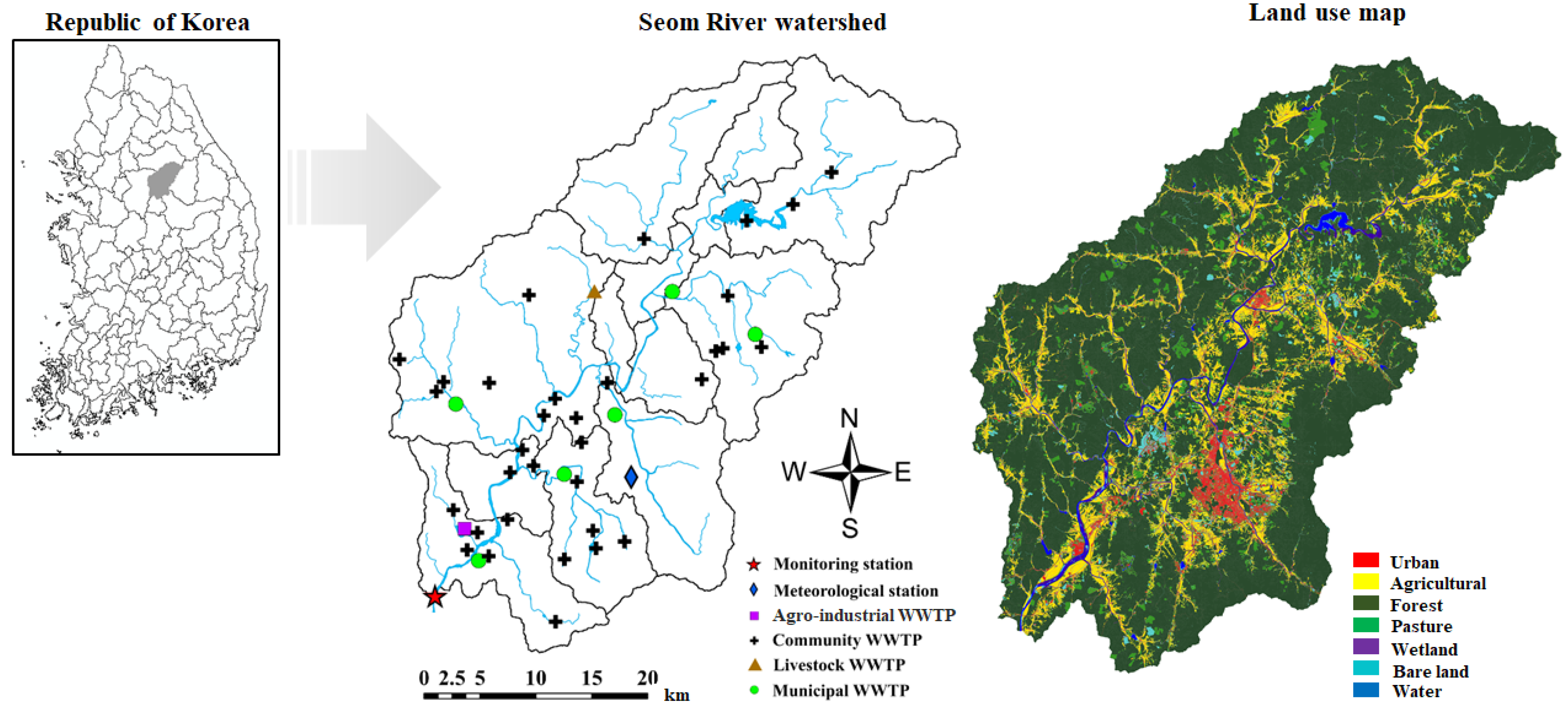
The study area was the Seom River watershed in South Korea (Figure 1), which has an area of 1473 km2 and a total population of 380,000 [31]. The main stream of the Seom River watershed, the Seom River, is 67.3 km in length and discharges into the South Har River. The study area is in an Asian monsoon climate region and the average annual precipitation during 2011–2015 was 1345 mm, approximately 65% of which occurred from June to August.
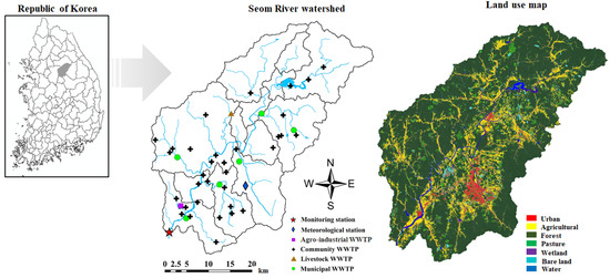
Figure 1.
Map of the Seom River watershed showing locations of point sources, meteorological stations, the monitoring station, and land use composition.
The Seom River watershed is largely covered by forests (75.63%) and agricultural land (17.21%), with a relatively small fraction (3.65%) of urban land (Figure 1). The NPS pollutants in the Seom River watershed include sediments and fertilizers, mainly produced from livestock farms and by agricultural activities. As of 2016, the total livestock population (cattle, pigs, and poultry) was 3,046,308 [32]. The PSs of pollution in the Seom River watershed are six municipal WWTPs (treatment capacity > 500 m3/d), 34 community WWTPS (treatment capacity ≤ 500 m3/d), three agro-industrial WWTPS, one WWTP in an industrial complex (mostly electronics and mechanical industries), and one livestock WWTP.
2.2. HSPF Model Configuration and Calibration
In our previous study, for improving the accuracy of a Chl-a simulation by HSPF [31], we replaced the original linear equation describing the temperature dependence of algal growth in HSPF with the following exponential equation (Equation (1)) to improve the prediction accuracy of Chl-a concentration:
where is the temperature correction factor for algal growth (0–1), Tw is the water temperature (in degrees Celsius), Tlb is the lower temperature limit for algal growth, Topt is the optimal temperature for algal growth, and Tub is the upper temperature limit for algal growth. The exponential equation describing the temperature–growth relationship has been shown to be more efficient than the original linear equation in replicating excess growth of phytoplankton during the summer season [31]. Our input data for the HSPF model were hourly timeseries data of meteorological variables recorded at the Wonju meteorological station, which is located in the study area [31]. The spatial data used to set up the HSPF were the most recent versions of the digital elevation model with a resolution of 30 m × 30 m and GIS layers of the watershed boundary, the stream network, and land uses provided by the Ministry of Environment (MOE), Korea [31]. The modified HSPF was automatically calibrated for flow, sediment, inorganic nutrients (PO43−-P, NO3−-N, and NH4−-N), and Chl-a at the watershed outlet by using a complex random factorization algorithm to minimize the root mean square errors between observed and simulated values. For the calibration, water quality and flow rate data at the outlet point (Figure 1) of the Seom River watershed were obtained from the MOE (http://water.nier.go.kr/web/waterMeasure?pMENU_NO=2, accessed on 3 March 2020). The flow rate data were the daily values of river discharge, and the water quality data comprised the water temperature (TW) and concentrations of Chl-a, phosphate (PO43−), nitrate (NO3−), ammonium (NH4+), total nitrogen (TN), total phosphorus (TP), and suspended solids (SS) measured at intervals of five to eight days [31]. Additional details on the HSPF modification, model configuration, and calibration procedure can be found in Lee et al.’s paper [31].
In the present work, the automatically calibrated model (“auto-calibrated model”) used in a previous study [31] was further tuned manually (“recalibrated”) for TP and TN, which were the target pollutants for source reduction. The auto-calibrated model underestimated the background level of phosphorous and Chl-a in the stream, although it simulated the excess algal growth well during summer seasons. For more accurate year-round simulations of phosphorous and Chl-a, the transport pathway of phosphorus from groundwater to the stream was introduced in the model (Figure 2), and the groundwater phosphorus concentration ranges for different land uses reported by various studies were considered during the recalibration [33,34,35,36,37]. Table 1 shows the groundwater soluble phosphorus concentrations obtained from the literature. The HSPF model was recalibrated for the period from 2011 to 2015 (2011–2013 for calibration and 2014–2015 for validation). The model performance was evaluated using the coefficient of determination (R2) and the percent bias (PBIAS), which can be defined as follows [38]:
where n is the number of data points in the timeseries, Ot is the observed value at time t, and St is the simulated value at time t. The R2 value ranges from 0 to 1, being more accurate as it approaches 1, and the accuracy of the model increases as the PBIAS approaches 0.
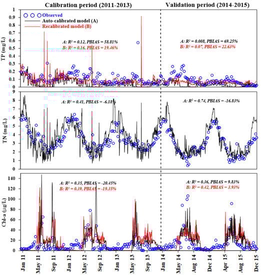
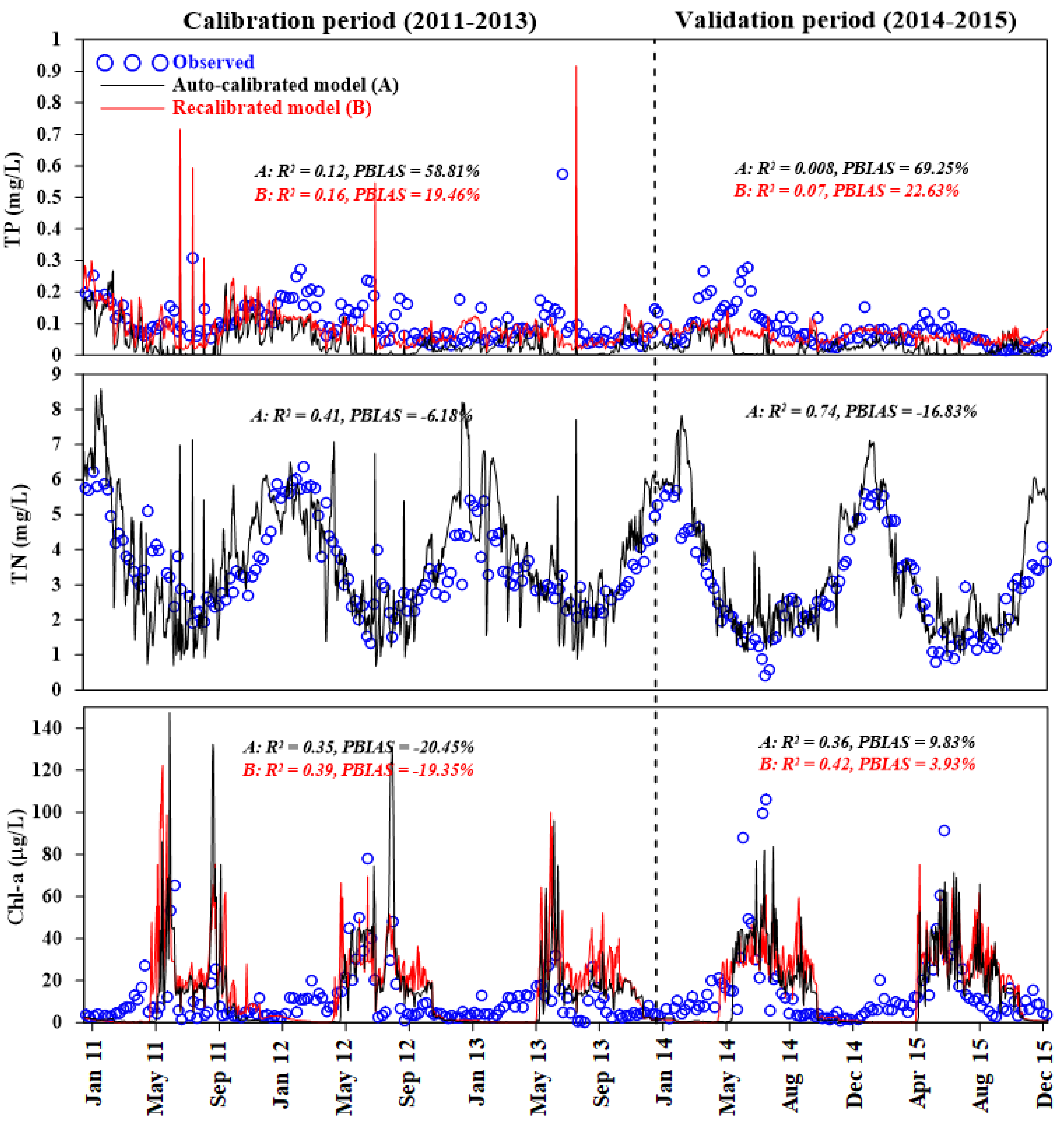
Figure 2.
Observed and simulated concentrations of total nitrogen (TN), total phosphorus (TP), and chlorophyll a (Chl-a). Black and red lines correspond to simulated values obtained with the auto-calibrated (A) and recalibrated models (B), respectively.

Table 1.
List of groundwater soluble phosphorus concentrations obtained from the literature.
The recalibrated HSPF model (“recalibrated model”) was used in a simulation to predict the Chl-a concentration at the watershed outlet from 2025 to 2050. Daily values of climate parameters such as precipitation, temperature, and solar radiation predicted from four different RCP climate change scenarios (“RCP scenarios”) were used in the simulation, and the effect of different pollutant reduction scenarios on the in-stream Chl-a concentration was simulated for different RCP scenarios. The BMPRAC module of the HSPF was used to incorporate NPS reduction scenarios for TN and TP discharged from lands with different uses for each sub-watershed.
2.3. Climate Change Scenarios
We used four RCP scenarios—RPC2.6, RPC4.5, RPC6.0, and RPC8.5—that represented greenhouse gas reduction scenarios reported in the Intergovernmental Panel on Climate Change Fifth Assessment Report [7]; the RCP numbers indicate the degree of greenhouse gas reduction, with a lower number reflecting a greater reduction effort (Table 2). The KMA has generated future climate data for South Korea for the RCP scenarios; the HadGEM2-AO and HadGEM3-RA models of the Met Office Hadley Centre for Climate Change Science and Services, UK, were used to generate global-scale (spatial resolution: 135 km) and Korea Peninsula-scale (spatial resolution: 12.5 km) climate data [39,40,41,42]. The Korean Peninsula-scale climate data were downscaled to obtain climate data for South Korea (spatial resolution: 1 km) by using a downscaling estimation model based on the Parameter-Elevation Regressions on Independent Slopes Model (PRISM) [43,44]. From the downscaled future climate data, KMA generated future climate data for each national meteorological station through bias correction and elevation adjustment. The future climate data used in this study comprised daily average wind speed (in meters per second), daily solar radiation (in watts per square meter), relative humidity (in percentage), daily average precipitation (in millimeters), daily average temperature (in degrees Celsius), daily maximum temperature (in degrees Celsius), and daily minimum temperature (in degrees Celsius).
Table 2.
Representative concentration pathway (RCP) climate change scenarios (Adapted from ref [7,14]).
2.4. Source Management Scenarios
Flow, nutrient loads, and Chl-a concentration in the absence of any source management practices were first simulated for the present (2011–2015) and future periods (2025–2050) for the RCP scenarios, and they were used as the basis for evaluating the effects of source management scenarios in the future. Three source management scenarios were considered (Table 3). Scenario 1 (S1) represented NPS control, which involved 50% reductions in both TP and TN loads from NPSs, including urban areas, agricultural areas, and grasslands. Urban and agricultural areas were considered as target land uses for management, because they are major contributors to NPS pollutant loads [45]. The proportion of grasslands in the Seom River watershed is relatively small (1.02%), and the grasslands include golf courses where a substantial amount of pesticides is applied. Accordingly, grasslands were selected as the target land use for NPS management. We assumed that the reduction in TN or TP sources on the land surface also decreased the levels of these pollutants in groundwater by the same degree. Therefore, in S1, the concentrations of TN and TP in groundwater and interflow runoff for the target land uses (i.e., urban and agricultural land) were assumed to be reduced by 50% to reflect source reductions from these land uses.
Table 3.
Source management scenarios.
Scenario 2 (S2) represented PS control, which involved the reduction in the TP concentration in the effluents of the six municipal WWTPs in the watershed to 0.1 mg/L. Although current effluent standards for WWTPs in Korea are different for different the water quality regions, the lowest numeric effluent standard for TP is 0.2 mg/L. Lake Biwa in Japan is often referred to as an excellent example of water quality improvement by enhancing the TP effluent standards for WWTPs [46,47]. Therefore, we considered the PS control scenario as a potentially effective measure for reducing algal blooms.
Scenario 3 (S3) represented both PS and NPS control. While NPS control was identical to that in S1, PS control differed from that in S2. In other words, the TP concentration in effluents of municipal WWTPs was limited to 0.1 mg/L only from May to September. During the crop growing season, nutrients are largely discharged from agricultural and urban areas because of agricultural activities and the use of pesticides for landscape management, increasing the level of nutrients in streams [31]. Thus, it is necessary to enhance nutrient control for both NPSs and PSs during the growing season. This season-based PS control strategy has been applied in San Diego, California, where the effluent standard for TP concentration is limited to 0.1 mg/L during the summer season [37,46,47].
3. Results
3.1. Model Performance
Figure 2 shows the simulation results obtained with the model calibrated for TN, TP, and Chl-a. The simulated TN values fitted the measured TN values well (R2 = 0.41 and PBIAS = −6.18% for calibration; R2 = 0.74 and PBIAS = −16.83% for validation). Furthermore, the simulated TN concentration showed the seasonal trends of the measured values. Concentrations of the nitrogen species in streams were generally higher during winter seasons, owing to the efficiency of biological nitrogen removal from WWTPs being lower at lower temperatures [48]. TN simulation results showed a background concentration of about 1 mg/L, partly reflecting the frequent nitrate contamination of the groundwater in Asian agricultural areas [49,50]. The TP concentration simulated using the auto-calibrated model was close to zero during summer seasons; this model could hardly capture the background TP level, which has a typical value in streams [51,52]. In the recalibrated model, the background concentrations in groundwater for different land uses were incorporated, and the simulation results were compared with those obtained with the auto-calibrated model in Figure 2. The performance ratings of both models for TP and Chl-a were “satisfactory” or better on the basis of the PBIAS values (|PBIAS| < 70% [38]), although the R2 values of these models were relatively low (R2 < 0.5). Compared with the auto-calibrated model, the simulated TP concentrations obtained with the recalibrated model fitted the observed values better, with the model showing superior performance in reproducing background TP concentrations; the values of R2 and PBIAS for TP obtained from the recalibrated model were 0.16 and 19.46% for calibration and 0.07 and 22.63% for validation, while those for TP acquired from the auto-calibrated model were 0.12 and 58.81% for calibration and 0.008 and 69.25% for validation. The recalibration for TP resulted in Chl-a also being recalibrated, since TP and Chl-a are strongly interconnected in the model structure (as phosphorus is the most important limiting nutrient for algal growth). As shown in Figure 2, the performance of the HSPF model improved after recalibration; the values of R2 and PBIAS for Chl-a for the recalibrated model were 0.39 and -19.35% for calibration and 0.42 and 3.93% for validation, while those for the auto-calibrated model were 0.35 and −20.45% for calibration and 0.36 and 9.83% for validation. While both the auto-calibrated and recalibrated models could simulate high Chl-a concentrations during summer seasons well, the performance of the recalibrated model was slightly better in replicating the base level of Chl-a during winter seasons.
3.2. Impact of Future Climate Changes on Algal Blooms
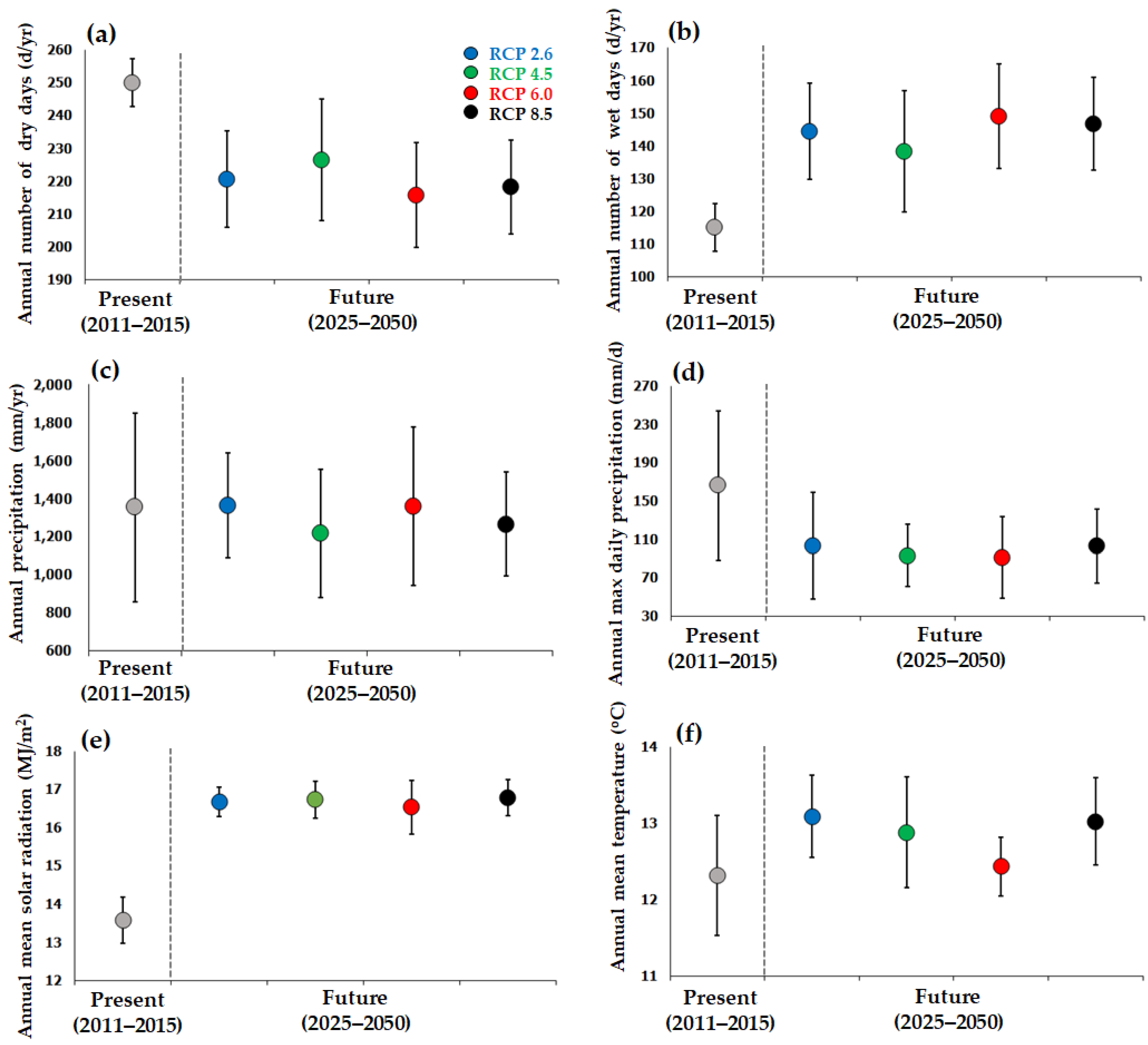
Figure 3 compares climate parameter values of the present period (2011–2015) with those of the future period (2025–2050) predicted by the KMA [7] for the four RCP scenarios downscaled for. The overall trend of the rainfall intensity in the Korean Peninsula was predicted to slightly increase owing to future climate changes, but large local variations and uncertainty exist in the prediction [53]. Furthermore, the surface temperature, solar radiation, and wet days in the Seom River watershed were predicted to increase. Interestingly, the maximum daily rainfall intensity is expected to decrease because of the increase in the number of wet days and little change in the annual total precipitation.
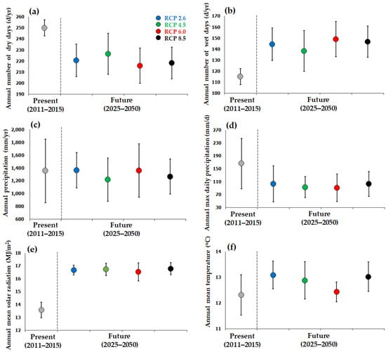
Figure 3.
Distributions of climate parameter values for the Seom River watershed simulated for the four climate change scenarios (RCP 2.6, RCP 4.5, RCP 6.0, and RCP 8.5) compared with those for the present period: (a) annual number of dry days, (b) annual number of wet days, (c) annual precipitation, (d) annual maximum daily precipitation, (e) annual mean solar radiation, and (f) annual mean temperature. The circle and error bar indicate the average and 1 standard deviation in the relevant periods, respectively.
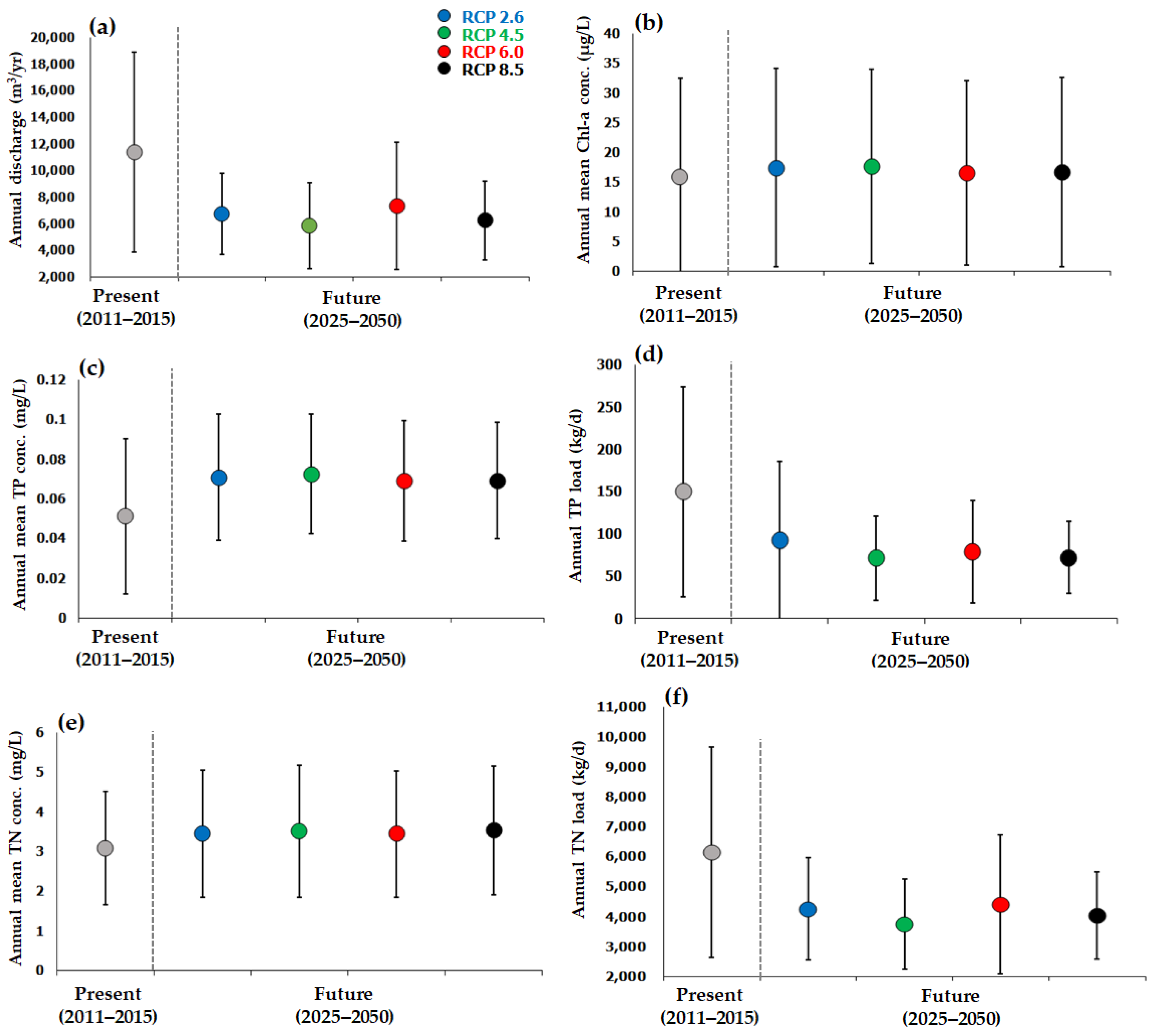
The recalibrated model was used for all the simulations with the RCP scenarios and pollutant reduction scenarios because of its better year-round performance in simulating TP and Chl-a compared with the auto-calibrated model. Figure 4 compares the simulated values of annual discharge, annual mean concentrations of Chl-a, TP, and TN, and annual mean loads of TP and TN between the present (2011–2015) and future periods (2025–2050).
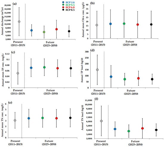
Figure 4.
Stream discharge, Chl-a concentration, nutrient concentrations, and nutrient loads simulated for the RCP climate change scenarios (the present period, RCP 2.6, RCP 4.5, RCP 6.0, and RCP 8.5): (a) annual discharge, (b) annual mean Chl-a concentration, (c) annual mean TP concentration, (d) annual TP load, (e) annual mean TN concentration, and (f) annual TN load. The circle and error bar indicate the average and 1 standard deviation in the relevant periods, respectively.
The annual discharge in the Seom River watershed was predicted to decrease by 35–49% in the future, largely because of a decrease in the rainfall intensity and the resulting decrease in the surface discharge. The annual mean loads of TP and TN were also predicted to decrease (by 39–52% for TP and 28–39% for TN), because the decrease in the rainfall intensity could significantly reduce the erosion and discharge of these pollutants from the land surface. By contrast, the annual mean TP and TN concentrations were predicted to increase (by 34–41% for TP and 12–14% for TN) because of a decrease in the stream water volume, resulting from the reduced discharge as well as increased evaporation.
The average and median values (not shown in Figure 4) of the simulated annual mean Chl-a concentration increased by 5–10% and 23–29%, respectively, compared with the values for the present period (median Chl-a = 13.1, 16.9, 16.9, 16.1, and 16.5 µg/L for the present period and for RCP 2.6, RCP 4.5, RCP 6.0, and RCP 8.0, respectively); little difference was observed in the mean Chl-a concentration and its annual variation among the RCP scenarios and between the present and future periods. The increased Chl-a concentration is probably because of increases in both nutrient concentrations and solar radiation. Among the RCP scenarios, there were no measurable differences or patterns in the simulated values of the hydrological and nutrient variables.
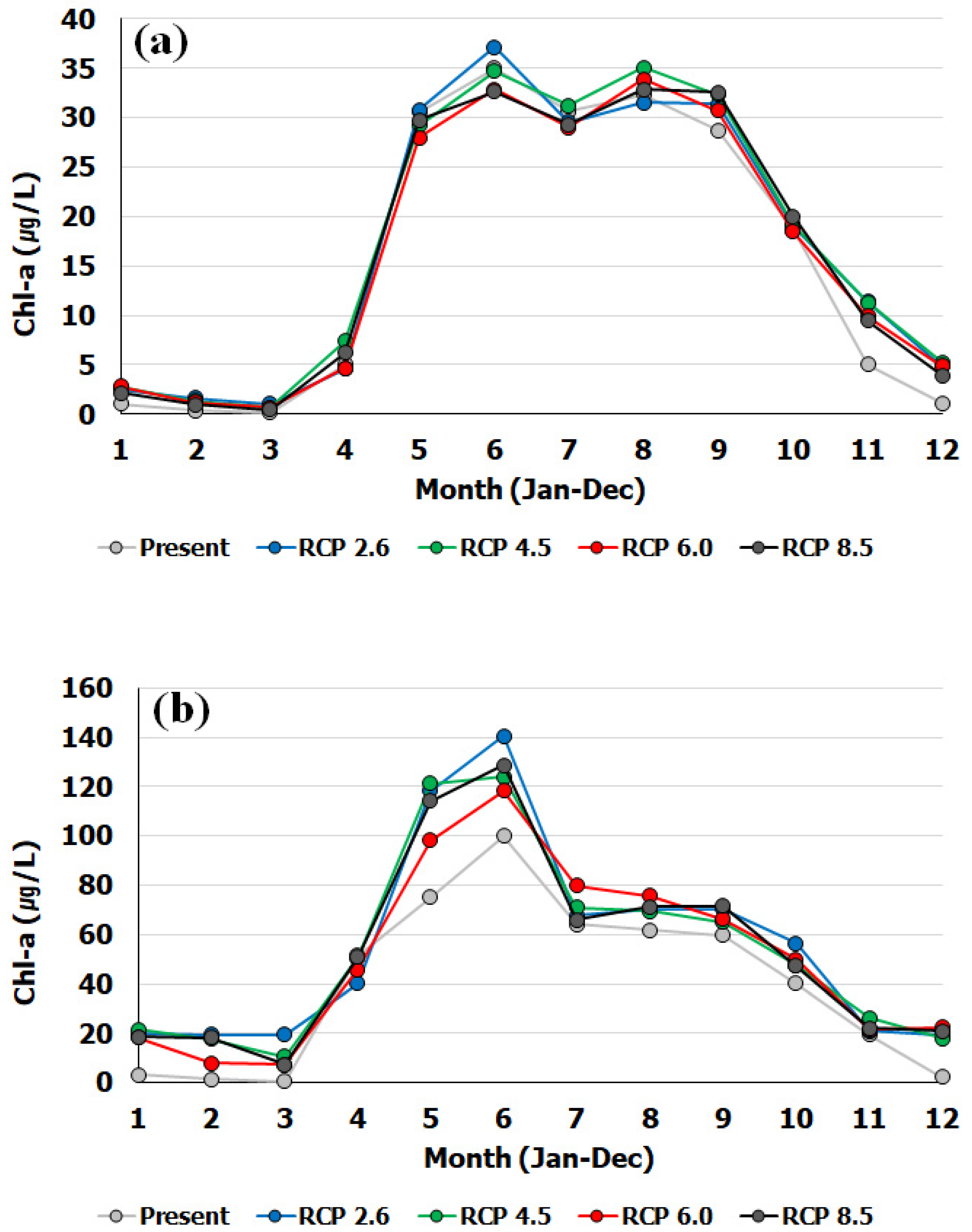
To examine the overall monthly variation of the Chl-a concentration in the present and future periods, we averaged monthly mean and maximum Chl-a concentrations for each simulated year over the simulated period for each scenario (Figure 5). As evident in Figure 5, there was little difference in the monthly mean Chl-a concentration among different RCP scenarios or between the present and future periods. However, the maximum Chl-a concentration was higher in the future period than in the present period, especially in May and June, implying a potential increase in algal blooms during summer seasons in the future. For all the RCP scenarios, the monthly mean Chl-a concentration from May to September exceeded 25 μg/L, which is the criterion for issuing a warning for potential algal outbreaks (hereafter termed “algal warning”) proposed by the MOE. These spring months are characterized by vigorous agricultural activities, which promote eutrophication and algal growth. The monthly maximum Chl-a concentration was the highest from May to June for all the RCP scenarios and simulation periods, indicating the impact of fertilizer application during the growing seasons in agricultural areas. Overall, the monthly mean and maximum Chl-a concentrations between May and September were higher than those for the other months, and for RCP 2.6, the simulated Chl-a concentration was relatively higher than those for the other scenarios, probably because of the higher annual maximum precipitation (Figure 3) and TP load (see Figure 4). For all the RCP scenarios, algal outbreaks were generally expected to occur in May and June. However, owing to large yearly variabilities in the predicted climate parameter values for all the RCP scenarios, minor patterns associated with the degree of greenhouse gas reduction (different RCP scenarios) were found in the Chl-a predictions.
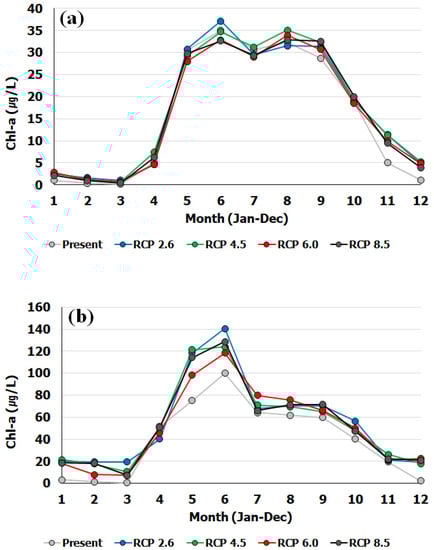
Figure 5.
(a) Monthly mean and (b) monthly maximum concentration of Chl-a during the present (2011–2015) and future (2025–2050) periods for different RCP climate change scenarios (RCP 2.6, RCP 4.5, RCP 6.0, and RCP 8.0).
3.3. Effects of Different Nutrient Source Management Strategies
Table 4 shows the reduction percentages (relative to the no management scenario) in the discharged TN and TP loads and the numbers of algal warning and algal outbreak cases at the outlet point of the watershed for different RCP scenarios. In this study, days with the Chl-a concentration exceeding 25 and 100 µg/L were defined as “algal warning” and “algal outbreak,” respectively, in accordance with the MOE’s recommendation. No monotonic trends were found in the algal warning and outbreak cases for different degrees of greenhouse gas reduction effort, probably because of the large temporal variability in the climate parameters predicted for the RCP scenarios.
Table 4.
Comparison of the effectiveness of different combinations of RCP and source management scenarios in reducing discharge loads of TN and TP and numbers of algal warning and outbreak cases.
The four RCP scenarios were compared with the no reduction scenario (“O”) in terms of nutrient discharge loads and the Chl-a concentration at the outlet point of the Seom River watershed. For all the RCP scenarios, the TN load at the outlet point was reduced by 11–12% for both nitrogen control scenarios (S1 and S3). The reduction in the TP load at the outlet point of the watershed ranged from 10% to 17% with few noticeable trends for different combinations of RCP and pollutant reduction scenarios; the reduction in the TP load was similar between S1 and S2 for all RCP scenarios, except for RCP 2.6. The TP load reduction for S3 was slightly greater than that for the other pollutant reduction scenarios.
The number of algal warning cases simulated for RCP 8.5 was the highest among the four RCP scenarios. Furthermore, RCP 2.6 always showed slightly better efficiency in reducing the number of algal warning cases compared with the other RCP scenarios. It predicted 18 algal outbreak cases, and it was followed by RCP 8.5 (15 cases), RCP 4.5 (12 cases), and RCP 6.0 (2 cases). RCP 2.6 showed the highest number of algal outbreaks, although it was the best scenario for limiting climate change; this observation contradicts the common belief that the largest reduction in the greenhouse gases would result in the best water quality in the future. This contradictory finding might result from the large variability and uncertainty in the climate change data forecast for the near future period preceding 2100 [54,55,56]. RCP 2.6 produced larger rainfall compared with the other RCP scenarios in the near future up to 2050 (see Figure 4) and larger numbers of potential algal outbreaks. This indicates that increased rainfall could increase the algal growth potential in streams because of an increase in NPS discharges. Despite this limitation, the HSPF simulation was useful for quantitatively comparing the effectiveness of different pollutant source management scenarios in preventing algal blooms.
For S1, the number of algal outbreaks could decrease by 20% to 58.3% for the RCP scenarios. However, S2 was superior to S1 in reducing the number of algal outbreaks (the reduction ranged from 44.4% to 100%). S1 and S2 were similar in reducing the number of algal outbreaks for RCP 2.6, while S2 was slightly more efficient than S1 for the other RCP scenarios. S3 completely prevented algal outbreaks in all RCP scenarios, except for RCP 2.6. These results imply that NPS control can offer greater efficiency in preventing algal growth for a climate change scenario that forecasts a larger number of algal outbreaks. Furthermore, for more efficient control of HABs, controlling PSs and NPSs by focusing on the summer season appears to be a cost-effective source management option.
4. Discussion
Although the performance ratings of the calibrated HSPF model for TN, TP, and Chl-a concentrations were better than or equal to the “satisfactory” level on the basis of the PBIAS rating criteria [34], R2 values between the observed and simulated TP and Chl-a concentrations were relatively low (0.07–0.16 for TP and 0.39–0.42 for Chl-a). These low R2 values were mainly because of the TP and Chl-a concentrations being underestimated during spring seasons, when significant discharge of phosphorous occurs because of season-specific rice farming in the study area [31]. Despite this underestimation of TP and Chl-a during spring seasons, the model captured the excess algal growth events during summer seasons reasonably well, which was the main focus of this study.
Although global climate change models predict overall increases in precipitation and stream discharge [14,53], the Seom River watershed is expected to experience a slight decrease in precipitation with increased frequency and decreased intensity, resulting in a net decrease in stream discharge and nutrient loads (Figure 3). However, the HSPF model predicted that algal blooms in the streams of the Seom River watershed would increase in the future owing to an increase in nutrient concentrations along with increases in the temperature and solar radiation (Figure 4). Thus, nutrient source control should effectively reduce the nutrient concentration in streams and thereby help reduce algal blooms.
Of the identified PSs in the Seom River watershed, the six municipal WWTPs were the major contributors to PS nutrient loadings, accounting for around 87% of the total TP load from PSs to the streams in the study area. Therefore, it would be more practical and cost effective to control only the effluents from the six municipal WWTPs (S1 and S3 scenarios in this study) than to control all the PSs dispersed across the watershed. Among the PS reduction scenarios presented in this study, the effectiveness of limiting the effluent TP concentration of WWTPs to 0.1 mg/L for improving stream water quality has been demonstrated in Japan and the USA in separate studies [46,47]. However, controlling PSs throughout the year might be costly, and hence, seasonally varying PS control along with NPS control is suggested in this study (i.e., S3). For example, chemical coagulation filtration can be additionally used in a WWTP as a tertiary treatment during the summer season.
According to our simulation, a 50% decrease in the effluent TP concentration (from 0.2 mg/L to 0.1 mg/L) for the six municipal WWTPs (S2) resulted in a slightly higher efficiency in reducing the Chl-a concentration in streams compared with the 50% reduction in TP and TN loads from NPSs (S1). However NPS control was still important to measurably reduce the excess algal growth, as evident in the simulation results of S3. In the Seom River watershed, the major NPSs are associated with urban and agricultural land uses that account for 3.65% and 17.21% of the entire watershed area, respectively. Agricultural land is predominantly located around the Seom River, and rice production is the main agricultural activity. During the spring–summer farming seasons, algal growth in the Seom River can be promoted by phosphorus and nitrogen discharged from the rice paddy fields adjacent to the streams. Accordingly, NPS control should be included as an important candidate management scenario for algal bloom control.
This study investigated the effectiveness of a 50% reduction in TP and TN loads from urban and agricultural land uses for controlling algal blooms in the future. To achieve a 50% reduction in NPS loads in agricultural areas, various structural and nonstructural NPS management techniques and their combinations can be used; examples are introducing regulations for adequate application of fertilizers/pesticides, using an improved irrigation drainage system, and employing nature-based management practices such as artificial wetlands, bio-retention basins, and riparian belts. A previous study conducted in Korea [57] reported removal efficiencies of 23.6% and 62.6% for TN and TP loads, respectively, by using an improved irrigation drainage system. One of the most efficient irrigation system improvements for rice paddy fields in Korea is known to be drainage outlet elevation, which involves raising the height of the paddy levee. It has been reported that drainage outlet elevation in a paddy field can increase the water storage capacity by 44% and lower the TP and TN discharge loads by 48.9% and 44.8%, respectively [58]. Another study conducted in Korea [57] reported that the reduction rates of TN and TP loads were 82.6% and 85.6%, respectively, when the water storage capacity of paddy fields was increased.
For urban areas, various NPS management techniques are available to reduce TP and TN loads by 50%. Conventional low-impact development (LID) facilities such as infiltration trenches, permeable pavements, green roofs, tree box filters, and bioswales can be used if land areas for their installation are available in urban areas. According to the guidelines for the installation and maintenance of LID facilities in Korea [59], the expected removal efficiencies of TN and TP loads for conventional LID facilities are 58–83% and 46–65%, respectively [59,60]. In the case of bioswales in Seattle, USA, a removal efficiency of 63% has been observed for both TN and TP loads [61].
The aforementioned agricultural and urban source management practices should be optimally designed and implemented on a watershed scale to attain the required reduction in the pollutant loads, given a limited budget and limited resources [59,60,62]. However, providing details of site-specific design and allocation strategies of the source management practices is beyond the scope of this study. These aspects should be examined in a future study.
5. Conclusions
The HSPF model was used with RCP climate change scenarios to predict HABs in the Seom River watershed from 2020 to 2050. To reduce algal blooms in the stream under future climate changes, three source management scenarios were evaluated: NPS control only, PS control only, and NPS and summer season PS control.
The simulation results showed that high algal biomass production will occur during the farming season (May to September) with the greatest potential of algal outbreaks likely to occur in the seeding season from May to June. It was found that in the study area, future climate change will increase the algal growth potential in streams because of an increase in the temperature and solar radiation and more frequent rainfall.
To effectively reduce algal blooms in the near future, controlling both PSs and NPSs would be necessary, but source management actions should focus on seasons when farming and seeding activities occur. In the study area, the most effective source management strategy was the control of both PSs and NPSs, which could almost completely prevent algal outbreaks, but this control strategy will be costly. Therefore, a season-based PS and NPS management strategy is proposed. PS control can be focused upon during growing seasons in May and June to reduce the cost of preventing algal blooms, without significantly compromising the prevention effectiveness. For example, season-based implementation of chemical tertiary treatment processes in major public WWTPs could help achieve the required PS reduction in the study area. To achieve the required NPS reduction, various stormwater management techniques and their combinations should be optimally implemented on a watershed scale. In particular, controlling nutrient discharge from agricultural land located near the streams can be important.
The watershed modeling approach used in this study can be useful to predict the stream water quality in response to future climate changes and source reduction and to thereby devise effective source management strategies and quantify management goals for specific pollutants such as phosphorus and nitrogen.
Author Contributions
All authors contributed to this study. Conceptualization: D.H.L., J.-H.K.; data analysis and investigation: D.H.L., P.S.F., J.H.K.; supervision: J.-H.K.; writing—original draft, D.H.L.; writing—revision and editing—D.H.L., J.-H.K. All authors have read and have agreed to the published version of the manuscript.
Funding
This work was supported by grants from the National Research Foundation (NRF) of Korea, funded by the Korean government (2018R1D1A1B07041093 and 2021R1A6A3A01087015).
Institutional Review Board Statement
Not applicable.
Informed Consent Statement
Not applicable.
Data Availability Statement
Not applicable.
Acknowledgments
This research was supported by a grant from National Research Foundation (NRF), funded by the Korea government (2018R1D1A1B07041093 and 2021R1A6A3A01087015).
Conflicts of Interest
The authors declare no conflict of interest.
References
- Smith, V.H.; Tilman, G.D.; Nekola, J.C. Eutrophication: Impacts of excess nutrient inputs on freshwater, marine, and terrestrial ecosystems. Environ. Pollut. 1999, 100, 179–196. [Google Scholar] [CrossRef]
- Lee, S.J.; Lee, S.E.; Kim, S.H.; Park, H.K.; Park, S.J.; Yum, K.T. Examination of critical factors related to summer chlorophyll a concentration in the Sueo Dam Reservoir, Republic of Korea. Environ. Eng. Sci. 2011, 29, 502–510. [Google Scholar] [CrossRef] [Green Version]
- Watson, S.B.; Whitton, B.A.; Higgins, S.A.; Paerl, H.W.; Brooks, B.; Wehr, J.D. Harmful algal blooms. In Freshwater Algae of North America; Wehr, J.D., Robert, G., Sheath, R.G., Kociolek, J.P., Eds.; Academic Press: San Diego, CA, USA, 2015; pp. 873–920. [Google Scholar]
- Noges, P.; Mischke, U.; Laugaste, R.; Solimini, A. Analysis of changes over 44 years in the phytoplankton of Lake Vrtsjarv (Estonia): The effect of nutrients, climate and the investigator on phytoplankton-based water quality indices. Hydrobiologia 2010, 646, 33–48. [Google Scholar] [CrossRef]
- Carey, C.; Ewing, H.; Cottingham, K.; Weathers, K.; Thomas, R.; Haney, J. Occurrence, toxicity, and potential ecological consequences of the cyanobacterium Gloeotrichia echinulata for low-nutrient lakes in the northeastern United States. Aquat. Ecol. 2012, 46, 395–409. [Google Scholar] [CrossRef]
- Paerl, H.W.; Paul, V.J. Climate change: Links to global expansion of harmful cyanobacteria. Water Res. 2012, 46, 1349–1363. [Google Scholar] [CrossRef]
- KMA. Climate Change Prediction in Korean Peninsula; Korea Meteorological Administration: Seoul, Korea, 2018; GPRN: 11-1360000-001555-01. [Google Scholar]
- Fu, F.X.; Tatters, A.O.; Hutchins, D.A. Global change and the future of harmful algal blooms in the ocean. Mar. Ecol. Prog. Ser. 2012, 470, 207–233. [Google Scholar] [CrossRef] [Green Version]
- Fee, E.J.; Hecky, R.E.; Kasian, S.E.M.; Cruikshank, D.R. Effects of lake size, water clarity, and climatic variability on mixing depths in Canadian Shield lakes. Limnol. Oceanogr. 1996, 41, 912–920. [Google Scholar] [CrossRef]
- Schindler, D.W. Widespread effects of climatic warming on freshwater ecosystems in North America. Hydrol. Process. 1997, 11, 1043–1067. [Google Scholar] [CrossRef]
- Magnuson, J.J. Potential effects of climate changes on aquatic systems: Laurentian Great Lakes and Precambrian Shield Region. Hydrol. Process. 1997, 11, 825–871. [Google Scholar] [CrossRef]
- NIER. Groundwater Background Quality Monitoring of Livestock Raising Area; National Institute of Environmental Research: Incheon, Korea, 2013. [Google Scholar]
- Paerl, H.W.; Huisman, J. Climate change: A catalyst for global expansion of harmful cyanobacterial blooms. Eviron. Microb. Rep. 2009, 1, 27–37. [Google Scholar] [CrossRef]
- IPCC. Climate change 2014: Synthesis Report. Contribution of Working Groups Ⅰ, Ⅱ and Ⅲ to the Fifth Assessment Report of the Intergovermental Panel on Climate Change; Core Writing Team, Pachauri, R.K., Meyer, L.A., Eds.; IPCC: Geneba, Switzerland, 2014; p. 151. [Google Scholar]
- Conley, D.J.; Paerl, H.W.; Howarth, R.W.; Boesch, D.F.; Seitzinger, S.P.; Havens, K.E.; Lancelot, C.; Likens, G.E. Controlling eutrophication: Nitrogen and phosphorus. Science 2009, 323, 1014–1015. [Google Scholar] [CrossRef]
- Dodds, W.K.; Smith, V.H. Nitrogen, phosphorus, and eutrophication in streams. Inland Waters 2016, 6, 155–164. [Google Scholar] [CrossRef]
- Ha, H.; Stenstrom, M.K. Identification of land use with water quality data in stormwater using a neural network. Water Res. 2003, 37, 4222–4230. [Google Scholar] [CrossRef]
- Lee, J.H.W.; Hodgkiss, I.J.; Wong, K.T.M.; Lam, I.H.Y. Real time observations of coastal algal blooms by an early warning system. Estuar. Coast. Shelf Sci. 2005, 65, 172–190. [Google Scholar] [CrossRef]
- Wagner, T.; Erickson, L.E. Sustainable management of eutrophic lakes and reservoirs. J. Environ. Prot. 2017, 8, 436–463. [Google Scholar] [CrossRef] [Green Version]
- Olaoye, I.; Confesor, R.; Ortiz, J. Impact of seasonal variation in climate on water quality of Old Woman Creek watershed Ohio using SWAT. Climate 2021, 9, 50. [Google Scholar] [CrossRef]
- Chung, E.; Park, K.; Lee, K.S. The relative impacts of climate change and urbanization on the hydrological response of a Korean urban watershed. Hydrol. Process. 2011, 25, 544–560. [Google Scholar] [CrossRef]
- Stern, M.; Flint, L.; Minear, J.; Flint, A.; Wright, S. Characterizing changes in streamflow and sediment supply in the Sacramento River Basin, California, using Hydrological Simulation Program—FORTRAN (HSPF). Water 2016, 8, 432. [Google Scholar] [CrossRef] [Green Version]
- Steenhuis, T.S.; Schneiderman, E.M.; Mukundan, R.; Hoang, L.; Moges, M.; Owens, E.M. Revisiting SWAT as a saturation excess runoff model. Water 2019, 11, 1427. [Google Scholar] [CrossRef] [Green Version]
- Arnold, J.G.; Moriasi, D.N.; Gassman, P.W.; Abbaspour, K.C.; White, M.J.; Srinivasan, R.; Santhi, C.; van Harmel, R.D.; van Griensven, A.; van Liew, M.W.; et al. SWAT: Model use, calibration, and validation. Trans. ASABE 2012, 55, 1491–1508. [Google Scholar] [CrossRef]
- Nasr, A.; Bruen, M.; Jordan, P.; Moles, R.; Kiely, G.; Byrne, P. A comparison of SWAT HSPF and SHETRAN/GOPC for modelling phosphorus export from three catchments in Ireland. Water Res. 2007, 41, 1065–1073. [Google Scholar] [CrossRef] [Green Version]
- Im, S.J.; Brannan, K.M.; Mostaghimi, S.; Kim, S.M. Comparison of HSPF and SWAT models performance for runoff and sediment yield prediction. J. Environ. Sci. Health Part A: Environ. Sci. Eng. 2007, 42, 1561–1570. [Google Scholar] [CrossRef] [PubMed]
- Xie, H.; Lian, Y. Uncertainty-based evaluation and comparison of SWAT and HSPF applications to the Illinois River Basin. J. Hydrol. 2013, 481, 119–131. [Google Scholar] [CrossRef]
- Albek, M.; Ogutveren, U.B.; Albek, E. Hydrological modeling of Seydi Suyu watershed (Turkey) with HSPF. J. Hydrol. 2004, 285, 260–271. [Google Scholar] [CrossRef]
- Göncü, S.; Albek, E. Modeling climate change effects on streams and reservoirs with HSPF. Water Resour. Manag. 2010, 24, 707–726. [Google Scholar] [CrossRef]
- Park, J.H.; Jung, E.T.; Jung, I.G.; Cho, J.P. Does future climate bring greater streamflow simulated by the HSPF model to South Korea? Water 2020, 12, 1884. [Google Scholar] [CrossRef]
- Lee, D.H.; Kim, J.H.; Park, M.H.; Stenstrom, M.K.; Kang, J.H. Automatic calibration and improvements on an in stream chlorophyll a simulation in the HSPF model. Ecol. Model. 2020, 415, 108835. [Google Scholar] [CrossRef]
- NIER. 2017 National Pollutant Source Survey Report; National Institute of Environmental Research: Incheon, Korea, 2019; GPRN: 11-1480523-00429-19. [Google Scholar]
- Carlyle, G.C.; Hill, A.R. Groundwater phosphate dynamics in a river riparian zone: Effects of hydrologic flowpaths, lithology and redox chemistry. J. Hydrol. 2001, 247, 151–168. [Google Scholar] [CrossRef]
- Holman, I.P.; Howden, N.J.K.; Bellamy, P.; Willby, N. An assessment of the risk to surface water ecosystems of groundwater-P in the UK and Ireland. Sci. Total Environ. 2010, 408, 1847–1857. [Google Scholar] [CrossRef] [Green Version]
- Jordan, T.E.; Correll, D.L.; Weller, D.E. Nutrient interception by a riparian forest receiving inputs from adjacent cropland. J. Environ. Qual. 1993, 22, 467–473. [Google Scholar] [CrossRef] [Green Version]
- Lewandowski, J.; Meinikmann, K.; Nützmann, G.; Rosenberry, D.O. Groundwater–the disregarded component in lake water and nutrient budgets. Part 2: Effects of groundwater on nutrients. Hydrol. Process. 2015, 29, 2922–2955. [Google Scholar] [CrossRef]
- Kim, G.H.; Yoon, J.Y.; Park, K.J.; Baek, J.H.; Kim, Y.J. Quantification of baseflow contribution to nutrient export from a agricultural watershed. Hydrol. Process. 2015, 29, 2922–2955. [Google Scholar] [CrossRef]
- Moriasi, D.N.; Arnold, J.G.; van Liew, M.W.; Bingner, R.L.; Harmel, R.D.; Veith, T.L. Model evaluation guidelines for systematic quantification of accuracy in watershed simulation. Trans. ASAE 2007, 50, 885–900. [Google Scholar] [CrossRef]
- Giorgi, F.; Coppola, E.; Solmon, F.; Mariotti, L.; Sylla, M.B.; Bi, X.; Elguindi, N.; Diro, G.T.; Nair, V.; Giuliani, G.; et al. RegCM4: Model description and preliminary tests over multiple CORDEX domains. Clim. Res. 2012, 52, 7–29. [Google Scholar] [CrossRef] [Green Version]
- Juang, H.M.H.; Hong, S.Y.; Kanamitsu, M. The NCEP regional spectral model: An update. Bull. Amer. Meteor. Soc. 1997, 78, 2125–2143. [Google Scholar] [CrossRef] [Green Version]
- Kang, H.S.; Cha, D.H.; Lee, D.K. Evaluation of the mesoscale model/land surface model (MM5=LSM) coupled model for East Asian summer monsoon simulations. J. Geophys. Res. 2005, 110, D10105. [Google Scholar] [CrossRef] [Green Version]
- Skamarock, W.C.; Klemp, J.B.; Dudhia, J.; Gill, D.O.; Barker, D.M.; Wang, W.; Powers, J.G. A Description of the Advanced Research WRF Version 2; NCAR Tech. Note; NCAR/TN 468+STR; National Center for Atmospheric Research: Boulder, CO, USA, 2005; p. 100. [Google Scholar]
- Kim, M.K.; Han, M.S.; Jang, D.H.; Baek, S.G.; Lee, W.S.; Kim, Y.H.; Kim, S. Production technique of observation grid data of 1km resolution. J. Clim. Res. 2012, 7, 55–68. [Google Scholar]
- Kim, M.K.; Lee, D.H.; Kim, J.N. Production and validation of daily grid data with 1km resolution in South Korea. J. Clim. Res. 2013, 7, 138–147. [Google Scholar]
- Lee, D.H.; Kim, J.H.; Mendoza, J.A.; Lee, C.H.; Kang, J.H. Characterization and source identification of pollutants in runoff from a mixed land use watershed using ordination analyses. Environ. Sci. Pollut. Res. 2016, 23, 9774–9790. [Google Scholar] [CrossRef]
- Han, M.D.; Park, B.K.; Park, J.H.; Kim, Y.S.; Rhew, D.H. Introduction of the basin sewerage plan in Japan through case studies of the Lake Biwa sewerage system. J. Korean Soc. Environ. Eng. 2015, 37, 533–541. [Google Scholar] [CrossRef]
- Sedlak, R.I. Phosphorus and Nitrogen Removal from Municipal Wastewater; CRC Press Taylor & Franeis Group: Boca Raton, FL, USA, 1991. [Google Scholar]
- Skoczko, I.; Struk-Sokołowska, J.; Ofman, P. Seasonal changes in nitrogen, phosphorus, BOD and COD removal in Bystre wastewater treatment plant. J. Ecol. Eng. 2017, 18, 185–191. [Google Scholar] [CrossRef]
- Jeon, S.R.; Jung, S.K.; Lee, Y.U.; Chung, J.I. Hydro geochemical characteristics and estimation of nitrate contamination sources of groundwater in the Sunchang area. Korea. J. Geo. Soc. Korea. 2011, 47, 185–197. [Google Scholar]
- Liu, J.; Jiang, L.H.; Zhang, C.J.; Li, P.; Zhao, T.K. Nitrate-nitrogen contamination in groundwater: Spatiotemporal variation and driving factors under cropland in Shandong Province, China. In IOP Conference Series: Earth and Environmental Science; IOP Publishing: Bristol, UK, 2017; Volume 82, p. 12059. [Google Scholar]
- Gardner, L.R. The role of rock weathering in the phosphorus budget of terrestrial watersheds. Biogeochemistry 1990, 11, 97–110. [Google Scholar] [CrossRef]
- Tipping, E.; Benham, S.; Boyle, J.F.; Crow, P.; Davies, J.; Fischer, U.; Guyatt, H.; Helliwell, R.; Jackson-Blake, L.; Lawlor, A.J.; et al. Atmospheric deposition of phosphorus to land and freshwater. Environ. Sci. Process. Impacts 2014, 16, 1608–1617. [Google Scholar] [CrossRef] [PubMed] [Green Version]
- KMA. Korean Climate Change Assessment Report 2020; Korea Meteorological Administration: Seoul, Korea, 2020; GPRN: 11-1480000-001692-01. [Google Scholar]
- Gelfan, A.; Gustafsson, D.; Motovilov, Y.; Arheimer, B.; Kalugin, A.; Krylenko, I.; Lavrenov, A. Climate change impact on the water regime of two great Arctic rivers: Modeling and uncertainty issues. Clim. Chang. 2016, 141, 499–515. [Google Scholar] [CrossRef]
- Hosseinzadehtalaei, P.; Tabari, H.; Willems, P. Uncertainty assessment for climate change impact on intense precipitation: How many model runs do we need? Int. J. Climatol. 2017, 37, 1105–1117. [Google Scholar] [CrossRef] [Green Version]
- Mirdashtvan, M.; Najafinejad, A.; Malekian, A.; Sa’doddin, A.J.M.A. Downscaling the contribution to uncertainty in climate-change assessments: Representative concentration pathway (RCP) scenarios for the South Alborz Range, Iran. R. Meteorol. Soc. 2018, 25, 414–422. [Google Scholar] [CrossRef]
- NIAS. Characteristics of Agricultural Non-Point Source Pollution Discharge and Development of Its Integrated Management Practice; National Institute of Agricultural Sciences: Wanju-gun, Korea, 2015; PJ008507. [Google Scholar]
- Rural Development and Economics Research (RDER). The Environment-Friendly Agricultural Infrastructure Improvement Plan to Reduce the Influence Agricultural Drainage on Water Pollution: Focus on the Paddy Field; RDER: Ansan, Korea, 2003. [Google Scholar]
- Ministry of Environment. Manual for Management of Reduction Facilities of Non-point Source Pollutions; Ministry of Environment: Sejong, Korea, 2020; GPRN: 11-1480000-001700-14.
- Ministry of Environment. Plan for Total Water Pollution Management; Ministry of Environment: Sejong-si, Korea, 2019; GPRN: NIER-GP-2019-010, 11-1480523-003731-14.
- USA EPA. Effectiveness of Low Impact Development; USA EPA: Washington, DC, USA, 2012.
- Ahiablame, L.M.; Engel, B.A.; Chaubey, I. Effectiveness of low impact development practices: Literature review and suggestions for future research. Water Air Soil Pollut. 2012, 223, 4253–4273. [Google Scholar] [CrossRef]
Publisher’s Note: MDPI stays neutral with regard to jurisdictional claims in published maps and institutional affiliations. |
© 2021 by the authors. Licensee MDPI, Basel, Switzerland. This article is an open access article distributed under the terms and conditions of the Creative Commons Attribution (CC BY) license (https://creativecommons.org/licenses/by/4.0/).