Abstract
By creating new job opportunities and developing the regional economy, the transport of goods generates significant costs, environmental and sanitary nuisances, and high greenhouse gas (GHG) emissions. In this context, collaboration is an interesting solution that can be used to enable companies to overcome some problems such as globalization, economic crisis, health crisis, issues related to sustainability, etc. This study deals with the design of a multiperiod multiproduct three-echelon collaborative distribution network with a heterogeneous fleet. By applying the mixed integer linear problem (MILP) formulations, it was possible to study the three dimensions of sustainability (economic, environmental, and social/societal). Since the examined problem was NP-hard, it was solved using four metaheuristic approaches to minimize the different logistics costs or CO2 emissions. The social/societal aspect evaluated the accident rate and the noise level generated by the freight transport. Four algorithms were developed to achieve our objectives: a genetic algorithm, a simulated annealing, a particle swarm algorithm, and a vibration damping optimization algorithm. Considering a French distribution network, these algorithms overcame the limits of the exact solution method by obtaining optimal solutions with reasonable execution time.
1. Introduction
In 2019, 374 billion ton-kilometers of goods were transported in the French metropolitan territory (including 11.8 billion by pipelines), a growth of 2.5% compared to 2018 [1]. These statistics show and highlight the importance of freight transport. However, it negatively influences the three main sustainability levels by increasing the logistics costs, the CO2 emissions, the depletion of nonrenewable resources, and the degradation of human life. Therefore, improving the effectiveness of the logistics operations by optimizing the distribution networks has been proved to be the best solution to face the companies’ difficulties. This effectiveness cannot be attained only by collaboration between companies. This strategy is the cornerstone of managing an efficient supply chain. It reduces, on the one hand, greenhouse gases, pollution, and congestion and, on the other hand, costs. In addition, it allows the agility and resilience of a company [2]. According to Aloui et al. [3], collaboration can be vertical (VC), horizontal (HC), and lateral. The VC is defined as a commercial agreement between two partners or more, from different levels of the network, in order to work together to take advantage of cooperation [4]. These partners (e.g., suppliers and clients) share important information about demands, deliveries, capacity, etc. However, the HC is based on sharing logistical resources between competitive partners who are at the same level of the network, but they belong to different logistics chains [5]. This type of collaboration improves the sustainability aspects through the reduction in logistics costs and CO2 emissions and the enhancement of the well-being of citizens and inhabitants, etc. [6,7]. Finally, lateral collaboration can be considered as the combination of the two other types of collaboration. As stated in Pan et al. [8], most studies deal with vertical collaboration, yet the results can be further enhanced through horizontal collaboration. Therefore, we are interested in the HC assuming that each partner applies a VC with its customers by sharing information. The problems covered by the HC can be classified according to the three levels of decision making: strategic, tactical, and operational [9]. The strategic level purpose is to satisfy the market demands. It often concerns long-term decisions, and it is difficult to change [10]. Among the strategic decisions, we can mention the design of distribution networks and the selection of partners [11]. On the other hand, the tactical level concerns the decisions in the medium-term. These decisions make it possible to satisfy predictable demands at the lowest production cost. Generally, they treat problems related to resource management, especially the problem of planning activities and the modalities of movement of goods in the structure designed at the strategic level. As instances of these decisions, we may cite the vehicle routing problem and the problem of sharing costs and CO2 emissions between partners [12]. Finally, the operational level concerns decisions that ensure the management of the means, the daily operation, and the flexibility of the supply chain in the short-term (the choice of the delivery and transport schedule, the allocation of transport means to sites, route selection, etc.) [13].
In this study, we are interested in the horizontal collaboration that improves the different sustainability levels. One of the main problems studied by the HC is the design of the collaborative distribution networks. Indeed, it is essential to address this problem by minimizing the impact of the different partners on the sustainability by reducing the logistics costs, CO2 emissions, accident rate and noise level, enhancing the filling rate, minimizing the travelled distances, etc.
The main contributions of this paper are the following: We propose four metaheuristics to efficiently solve our distribution problem. A genetic algorithm (GA), a simulated annealing (SA), a particle swarm algorithm (PSO), and a vibration damping optimization (VDO) were introduced with an encoding adapted to our problem. In particular, the latter is NP-hard and its exact mathematical resolution is limited in terms of computing time. Thus, it is necessary to develop metaheuristic algorithms to find approximate solutions with a minimum gap in an acceptable resolution time. Moreover, we treated two different collaborative scenarios with different distribution policies. The parameters of our proposed algorithms were set via a typical experimental method. Furthermore, our objectives were to minimize the logistics costs or the CO2 emissions and evaluate the noise level and the accident risk. To assess the effectiveness of the introduced algorithms, the latter were tested on a fictitious distribution network. A sensitivity analysis was performed to explore the impact of the problem’s size on the results through extensive computational experiments that were performed on different instances to validate our proposals.
The remainder of the paper is organized as follows. Section 2 presents a literature review about the resolution methods used in distribution networks. Section 3 introduces the mathematical model, its description, and formulation. Section 4 describes the proposed metaheuristics. Section 5 reports the experimental results of the case study. Section 6 presents the sensitivity analysis. Finally, Section 7 provides the conclusion and future work.
2. Literature Review
The distribution network design problem (DNDP) objectives are: (i) to identify the optimal strategy (number and location of hubs), (ii) assign non-hub nodes (suppliers, customers, etc.) to hubs, and (iii) determine the links between hubs and logistics routes [14]. According to O’Kelly [15], the DNDP can be defined as a general hub location problem (HLP). Following the landmark studies of [16,17], HLP has been well studied in the literature [18,19,20,21]. Considering the cost or time in the objective function, the HLP can be divided into the hub median problem (HMP) and the hub center problem (HCP) (See [22,23]). Based on the type of allocation of non-hub nodes to hubs, we can distinguish two types of allocation. In the case where a non-hub node is assigned to multiple hubs, we talk about multiple allocation. However, when a non-hub node is allocated to a single hub, the allocation type will be single allocation. Mathematical models dealing with HLP are NP-hard and their exact resolution is limited in terms of computing time. Thus, it is necessary to develop heuristic algorithms to find approximate solutions with a minimal gap during an acceptable resolution time. For this reason, Rodríguez et al. [24] developed a simulated annealing (SA) algorithm to study hub location problems with hubs’ capacity constraints (CSAHLP). The proposed SA algorithm provided better solutions and improved the level of service. In addition, Kratica et al. [25] examined an uncapacitated single allocation p-hub location problem (USAp-HLP) with two evolutionary metaheuristics. Both genetic approaches were introduced to solve the problem using new coding schemes and modified genetic operators. The obtained results showed that the proposed approaches achieved all the optimal solutions, even for large-sized problems. However, Randall [26] examined a CSAHLP. They implemented an ant colony optimization metaheuristic (ACO) to determine optimal solutions in a reasonable computing time. In addition, Ilić et al. [27] studied an USAp-HLP with economic objectives. As the number of constraints and variables increased exponentially with the size of the problem, a general variable neighborhood search (GVNS) was employed to overcome the limitations of exact methods. The findings provided by the GVNS were compared with those obtained by other heuristics and the efficiency of this method in reducing the computational time was proven. Nonetheless, Stanimirović et al. [28] presented a GA to address a capacitated single allocation p-hub location problem (CSAp-HLP). Binary coding of individuals and modified genetic operators were also used to solve the problem. Thus, the GA was proved to be effective in dealing with large-sized problems which cannot be solved with exact methods. On the other hand, Lin et al. [29] studied a capacitated multiple allocation p-hub location problem (CMAp-HLP). They solved this problem applying a GA to overcome the limitations of the mathematical model. In return, Yang et al. [30] proposed a hybrid algorithm to deal with an USAp-HLP. This algorithm (GA-LS), which incorporated the GA and local search (LS), showed better performance, compared to the classical version of the GA. The authors developed another hybrid algorithm (PSO-LS) where the PSO and the LS [31] were combined. PSO-LS was more efficient than the PSO and the GA in terms of quality, solutions, and execution time. Similarly, Ghaderi and Rahmaniani [32] proposed two hybrid metaheuristics based on PSO and VNS combined with the tabu search (TS) to solve the studied problem. Comparing the introduced solutions with those obtained with CPLEX, the two hybrid methods performed well, for all instances, in terms of computational efficiency and solution quality. In addition, two metaheuristics (SA and iterated local search (ILS)) were proposed by Fazel Zarandi et al. [33] to reach optimal solutions in a more negligible computational time, compared to the exact resolution, and with a very high precision level. Moreover, Damgacioglu et al. [34] studied an uncapacitated single allocation hub location problem (USAHLP). They introduced a GA to solve their mathematical model in a reasonable time. The GA showed better results than the location–allocation algorithm and discrete solutions but in longer resolution time. A mixed integer programming model and a VNS algorithm were developed by Serper and Alumur [35] to examine a HLP with different types of vehicles. The VNS algorithm was able to find good quality solutions in a reasonable time. Furthermore, a mathematical formulation was introduced by Rabbani et al. [36] to solve an USAp-HLP. Due to the nonlinear nature of the proposed model, the authors applied a GA to overcome the limitations of the model and solve large-sized problems in a reasonable time. On the other hand, a capacitated multiple allocation hub location problem (CMAHLP) was studied by Mirabi and Seddighi [37] and a new hybrid algorithm based on ACO and SA was also proposed to solve this problem. The results of the mathematical model showed that the developed algorithm is efficient in solving the problem. Moreover, Neamatian Monemi et al. [38] introduced a collaborative mathematical model for an HLP between two logistics service providers. This model was very difficult to be solved, even for very small instances. The authors introduced a mathematical solution algorithm integrating lagrangian relaxation (LR) into a LS algorithm that could be used to obtain good and acceptable solutions. Nevertheless, Ghaffarinasab et al. [39] addressed the same problem but with the two allocation strategies (single and multiple). Mathematical formulations and algorithms based on SA were developed in order to study the related problem. Moreover, Bashiri et al. [40] presented a mathematical model to deal with multiperiodic HLP in a dynamic environment. The authors developed a GA with an LS method and a SA algorithm. They found that the GA was more efficient than the SA in dealing with real-world applications where demand is changing rapidly. Moreover, a mathematical model was proposed by Lüer-Villagra et al. [41] for an USAp-HLP. This model was difficult to solve, even for small instances. To overcome this weakness, the authors generated a GA that effectively and quickly solved the problem. At the same time, Özgün-Kibiroğlu et al. [42] suggested a mixed integer nonlinear programming (MINLP) formulation to solve an uncapacitated multiple allocation hub location problem (UMAHLP) using a PSO algorithm, which was applied to effectively solve the model. In addition, a HLP was studied by Shang et al. [43] with a stochastic programming model formulated in MILP to minimize distribution and opening costs. Due to the complexity of the computation, a memetic algorithm (MA) was introduced to solve the considered problem. This algorithm combined genetic research and LS to find optimal solutions within a reasonable computational time. Under these conditions, comparative results proved that the MA was more efficient than the GA in terms of the quality of solution and the speed of calculation. The same problem was addressed by Shang et al. [44] using a robust optimization model that enabled the attainment of economic goals. The authors proposed a VNS algorithm and a heuristic based on the population-and-searching (PAS) to find the optimal solutions. The obtained findings showed that the PAS algorithm was the most efficient in dealing with large instances, compared to the CPLEX software and the VNS algorithm. In addition, a GA was introduced by Wang et al. [45] to select the optimal hub locations and to ensure that the total network cost was minimized and products are delivered on time. The results demonstrated that the proposed algorithm could reduce the total cost and improve the efficiency of the network. The reviewed studies are summarized in Table 1.

Table 1.
Related papers.
From this table, we can see that, in most of the studies dealing with HLP, the objective function of the proposed metaheuristics was to minimize logistics costs (transportation, storage, opening, etc.). However, none of these research works considered the three sustainability levels when designing the distribution networks and not all introduced models were flexible in terms of the delivery time. For these reasons, we present, in this study, a model that addresses the economic level or the environmental level and evaluates the social/societal level. On the other hand, the platforms’ capacities, in most of the existing studies, were predefined, which led to a predefined opening cost that did not depend on the warehouse area. Thus, it would be more optimal to consider the capacity of each hub as a decision variable determined by the model depending on the quantity of goods entering each warehouse. In addition, as demonstrated in most studies, a homogeneous fleet of vehicles represents a weakness due to the variability of demand that requires a flexible (heterogeneous) fleet with variable types of vehicles to ensure the customer’s satisfaction. In this study, we use a heterogeneous fleet of vehicles that enabled modelling of the economy of scale. As stated in [35], the main reason for employing different types of vehicles in distribution networks is to achieve economies of scale and reduce the unit transportation cost by using larger-capacity vehicles. Therefore, we introduce, in this paper, meta-heuristic algorithms, namely a GA, a SA, a PSO and a VDO, to effectively solve the studied problem. The GA and the PSO were based on the population generation, which gives a larger research space. Moreover, the SA and the VDO are single solution algorithms and they offer low execution time.
3. Description and Formulation of the Problem
In this section, we examine a collaborative distribution network design problem that addresses three levels of sustainability. The targeted distribution network, shown in Figure 1, contains suppliers who collaborate to deliver multiple products to retailers through the shared warehouses and distribution centers. The distribution of these products is carried out in a multiperiodic way and with several types of vehicles, which makes the vehicle fleet heterogeneous. The problem is similar to the CS/MAp-HLP (capacitated single/multiple allocation p-hub location problem), which is solved in the strategic decision context. The problem has two main objectives. The first is to determine the number and locations of the two types of hubs (warehouses and distribution centers). On the other hand, the second aim consists in assigning suppliers and distribution centers to warehouses and retailers to distribution centers. Moreover, the mathematical model determines the capacities of hubs, which are limited and depend on the quantities of goods entering each hub, the quantities delivered in each period in the three parts of the network (upstream, intermediate and downstream), the level of stocks in the warehouses, the delayed quantities, and the number and type of the used vehicles. As the upstream hubs are supposed to have storage times, their role is to store goods. On the other hand, downstream hubs are like cross-docking platforms in the sense that they have no storage time. The main functions of these platforms are to sort goods and distribute them to retailers.
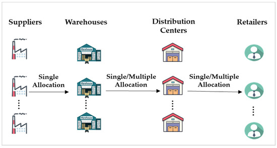
Figure 1.
Example of addressed distribution network.
Today, sustainability has become one of the most important challenges. Therefore, collaboration is one of the solutions that has proven its efficiency in achieving the main goals of sustainability. It allows partners to benefit from certain advantages that contribute to a green and sustainable distribution network by ensuring the massification of flows, grouping together goods, and sharing resources and means. The three levels of sustainability are assessed, in this study, by minimizing the logistics costs or the CO2 emissions and evaluating the noise levels and the risk of accidents. The evaluated sustainability indicators are shown in Figure 2.
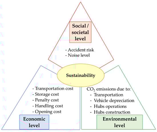
Figure 2.
Evaluated sustainability aspects.
The examined mathematical model was first proposed by Mrabti et al. [46]. It considered two scenarios (see Figure 3). The first scenario (Sc1) imposed that each supplier was assigned to a single warehouse (single allocation), which, could deliver to only one distribution center (single allocation), and each retailer could be assigned to several distribution centers (multiple allocation). However, the second scenario (Sc2) differed from the first one at the levels of the assignments of warehouses to the distribution centers, on the one hand, and retailers to distribution centers, on the other hand. Therefore, each warehouse can deliver multiple distribution centers (multiple allocation) and a retailer can only be assigned to one distribution center (single allocation).
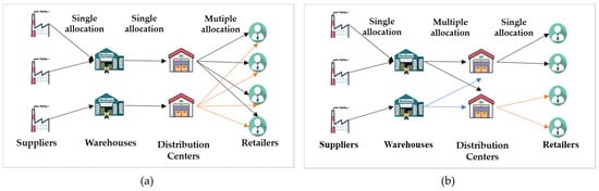
Figure 3.
Examined scenarios. (a) Scenario Sc1; (b) Scenario Sc2.
To formally introduce the studied problem, the following notations were used in the remainder of this study.
Sets
T1: Set of periods
P: Set of products
N: Set of suppliers
M: Set of warehouses
K: Set of distribution centers
J: Set of retailers
V: Set of vehicles
F: Set of nodes F =
H: Set of hubs H = M K
T2: Set of periods considering the flexibility in the delivery time:
T2 = T1 +
A1: Set of arcs in the upstream part between suppliers and warehouses
A2: Set of arcs in the midstream part between warehouses and distribution centers
A3: Set of arcs in the downstream part between distribution and retailers
A: Set of arcs A =
Parameters
: European pallet surface
: Quantity of product p requested by the retailer j in period t
: Safety stock of product p in hub m
: Unit transport cost of fully-loaded v-type vehicle
: Unit transport cost of an empty v-type vehicle
: Distances travelled between origin i and destination j
: Transportation cost between origin i and destination j by v-type vehicle at period t
: Storage cost of product p in hub m at period t
: Unit storage cost of product p in hub m at period t
: Penalty cost of product p at period t
: Unit penalty cost of product p at period t
: Opening cost of hubs m
: Unit opening cost of hubs m
: Unit unloading cost of product p
: Unit loading cost of product p
: Unit sorting cost of product p
: Handling cost of product p in hub m at period t
: Coefficient greater than or equal to 2
Z: A large constant
: CO2 emissions from v-type vehicle, while travelling from origin i to destination j at period t
: Unit CO2 emissions from fully-loaded v-type vehicle
: Unit CO2 emissions due to empty v-type vehicle
: CO2 emissions due to the operation of hubs m at period t
: CO2 emissions due to the construction of hubs m
: Unit CO2 emissions due to the construction of hubs m
: CO2 emissions due to the manufacturing of v-type vehicle with depreciation
: Energy consumed by hub m at period t
, , and : Bodily, fatal and nonfatal Accident rate
Ac: Number of accidents caused by heavy vehicles
D: Total travelled distance
NL: Noise level
: Representative flows in light or heavy vehicles
V: Speed
d: Distance to the platform edge
lc: Width of the road
: Angle under which we see the road
: Flow rate of heavy goods vehicle that flows between origin i and destination j at the period t
: Noise level when transporting goods from origin i to destination j at the period t
: Percentage of mortality
: Acoustic equivalence factor between light and heavy vehicles
Variables
: Quantity of product p transported from origin i to destination j by the v-type vehicle at period t
: Inventory level of product p in hub m at period t
: Hub m capacity
: Number of v-type vehicles at period t between origin i and destination j
: Quantity of product p delayed in period t
: Hub m area
: Binary variable equals to 1, if the warehouse m is open, and to 0 otherwise
: Binary variable equals to 1, if there is a link between the two nodes i and j, and to 0 otherwise
: Binary variable equals to 1, if the retailer j is affected to the distribution center k, and to 0 otherwise
Considering the above-described notations, the problem dealing with scenario Sc1 was formulated as follows:
subject to
The economic objective function (1) minimized the logistics costs linked to transportation, storage, late delivery penalties, the establishment of hubs, and handling represented respectively by ((2), (3), (5), (7) and (9)). The inventory level in warehouse m was given by (4). The delayed amount of product p at period t was shown in (6). The initial delayed quantity was equal to zero. The area of a hub m to build was given by (8). The environmental objective function (10) minimized the various CO2 emissions due to vehicles (their manufacture and operation), represented by (11), and to hubs (their construction and operation) demonstrated by (12) and (13). The accident rate per thousand km was given by (14). The multiplication by two in (15) was done to consider the empty return. Knowing that an accident injury can be fatal or nonfatal, the other two accident levels (nonfatal injury and fatal injury) might be also assessed. The first level was given by (16). This mortality rate was determined from statistical reports on road safety in France. The rate of nonfatal accidents was given by (17). The noise level was obtained by (18). The acoustic equivalence changed depending on the degree of the ramp and the type of track. The route chosen by the authors was a motorway, which was a communication road with separate lanes reserved for the rapid circulation of motor vehicles (cars, motorcycles, and heavy goods vehicles). The motorway was made up of 4 express lanes (2 per direction); each of which had a width of 3.5 m. The distance to the platform edge, measured by meter, was defined as a distance between the edge of the road platform and the receiver (person and buildings, etc.). The receiving point was assumed to be 30 m from the road. As far as the speed was concerned, it was fixed at an average speed equal to 80 km/h. After simplification, (19) was used to evaluate the noise level generated by the distribution of goods. The flows of heavy goods vehicles were equal to the number of vehicles or the number of trips. They were given by formula (20). Constraints (21) and (22) ensured the satisfaction of the retailers. In fact, constraint (21) guaranteed that the sum of the quantities delivered by all the suppliers in period t and the stock level of the previous period must be greater than or equal to the quantity of goods delivered between the hubs. The initial inventory level was equal to zero. Constraint (22) ensured that the quantity of inter-hub goods delivered from the warehouse to the distribution center in each period must be exactly equal to the quantity delivered to retailers. Constraint (23) guaranteed the satisfaction of the requests during the authorized periods. Indeed, for each product, the demand of the retailers in each period must be delivered at most in period t + ap. In our case, ap designated the number of periods authorized to deliver the product p. In other words, this parameter designates the level of flexibility in terms of delivery time of each supplier. Constraint (24) indicated that the stock level of each product in the upstream hubs must not be lower than that of the safety stock. Constraint (25) showed that the incoming quantities must be less than the capacities of the hubs. Constraints (26) and (27) demonstrated that a warehouse was only open if, at least, one supplier was assigned to it and that a platform was only open if at least one warehouse was assigned to it. Parameter Z was equal to a large constant. Constraint (28) guaranteed that the number of platforms to be opened was always less than that of candidates. Constraint (29) was used to limit the flow of flows on the arcs. Indeed, no quantity of goods circulated between the nodes unless there was a link between them. Constraint (30) ensured that a supplier was assigned to a single warehouse. Constraint (31) revealed that a warehouse was assigned to a single distribution center. Constraint (32) determined the number of vehicles required to transport the goods on the three parts of the distribution network. Constraint (33) limited the number of vehicles used on each arc. Constraint (34) was employed to conserve flows. The last constraints (35)–(41) provided the domains of defining each decision variable.
The difference between the problem dealing with Sc2 and that dealing with Sc1 was summarized by the following equations:
Equation (42) ensured that each retailer was delivered by a single distribution center and (43) guaranteed that each shared warehouse could deliver goods to many distribution centers.
4. Solution Approach
Since the considered problem was NP-hard, it could not be resolved with traditional-solution approaches for large-sized instances, hence the importance of applying metaheuristic approaches. So, we introduce and describe the encoding plan of all the proposed metaheuristics.
4.1. Encoding Plan
To solve our studied problem, it is impossible to use traditional solutions. Generally, each problem has its own data structure and individuals, in the literature, are represented either by vectors [39] or by tables [47,48]. However, in this work, a candidate individual was represented by a set of tables; each of which showed a given period. There were two types of tables. The first type Af represented the links in the studied network. It was a table containing four rows associated respectively with the indices of the four network sets. The number of columns was the multiplication of the number of suppliers and retailers. The first row demonstrated the supplier indices, the second and third rows described warehouses and distribution centers, respectively, while the last line exposed retailers. This table was represented only once since the assignment did not change during the periods. For example, a simple case contained two suppliers, three warehouses, three distribution centers, and three retailers. These elements are shown in Figure 4 and the links of the example are described by part (A).
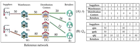
Figure 4.
Illustration of the proposed coding.
The second type Qty, which represented the product quantities to be transported between the suppliers and the retailers, was a table with the same size of Af. Each period had its own table since the requests were multiperiodic. It was assumed that the three retailers had the respective demands of products P1 and P2: {20 P1, 0 P2}, {18 P1, 0 P2}, and {12 P1, 80 P2}. Part (B) contained the type Qty of this solution and it is shown in Figure 4.
4.2. Meta-Heuristic Algorithms
4.2.1. Genetic Algorithm
The GA was first proposed by [49] and successfully used in various optimization problems. It mimics three genetic operations on a certain basic population (the selection, the mutation, and the crossover) to synthesize the best characteristics of different individuals. Genetic algorithms have been widely applied in the literature [30,34,36,40,41,50]. They are of great potential for practical applications. Indeed, genetic algorithms provide excellent performance at low costs. They make it possible to explore areas with many solutions. In addition, they use four elements to find the extrema(s) of a function defined on a data space. The pseudocode of GA is presented in Figure 5.
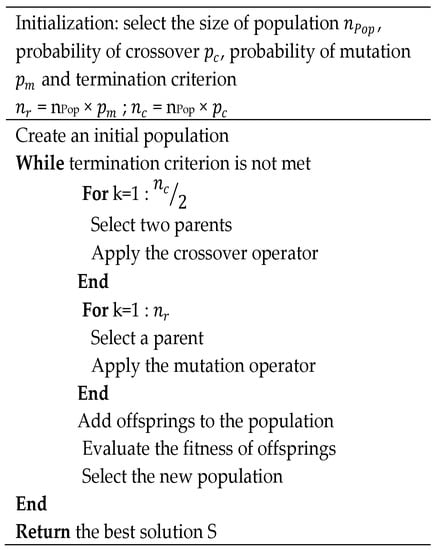
Figure 5.
Pseudocode of the used genetic algorithm.
When starting the genetic algorithm, the programmer must provide an initial population that respects the constraints of the studied problem. The algorithm starts by generating some initial solutions, which represent the initial population, from the search space in a random fashion. These solutions are presented in the form of chromosomes composed of several genes. The initial population plays an important role in the convergence of the final solution [51]. After generating the initial population, a score must be assigned to each individual to distinguish the most promising ones who will participate in the improvement of this population in future generations. At each iteration, the algorithm selects, from the current population, the individuals who will survive and reproduce to create an intermediate population. The selection phase is crucial in determining the performance and quality of the new generations. To diversify the population and explore the workspace, diversification operators are used across the succeeding generations. Among these operators, we cited the crossover and mutation operators. In fact, the purpose of the former is to exchange parts of the chains of two individuals, which allows the genetic mixing of the population. However, the mutation ensures the exploration of the workspace. The purpose of crossover is to enrich the diversity of the population by manipulating the structure of chromosomes. In general, crossovers occur between two parents to produce two offspring. The mutation operation allows the genetic algorithm to better scan the search space by modifying a gene. In our case, the mutation operator used various modifications.
4.2.2. Simulated Annealing
The SA, proposed by Kirkpatrick et al. [52], is a technique that solves optimization problems. It is a one-solution metaheuristic whose idea stems from the physical annealing process of maximizing the temperature of a metal until it melts. Then, cooling is carried out by lowering the temperature until the minimum energy is reached to obtain a stable crystalline structure. If the cooling rate is fast, the metal will be brittle. The SA consists in generating a random initial solution S, as explained in the following section, and looking at each iteration for a feasible neighboring solution S′. If the new solution is improved, an update of the solution is performed (S = S′). If not, the new solution can be accepted in order not to be trapped in a local minimum with a certain probability of acceptance represented by (44).
where f is the objective function and T denotes a temperature parameter.
A uniform random number p in the interval [0, 1] is generated. If p is less than the probability of acceptance, the new solution will be accepted. The chance of accepting poor quality solutions diminishes gradually. At each iteration, the temperature decreases regularly according to a cooling coefficient α such that T = α·T where α ∈ [0, 1]. The loop is repeated until a termination criterion is met. The pseudocode of the simulated annealing algorithm is shown in Figure 6.
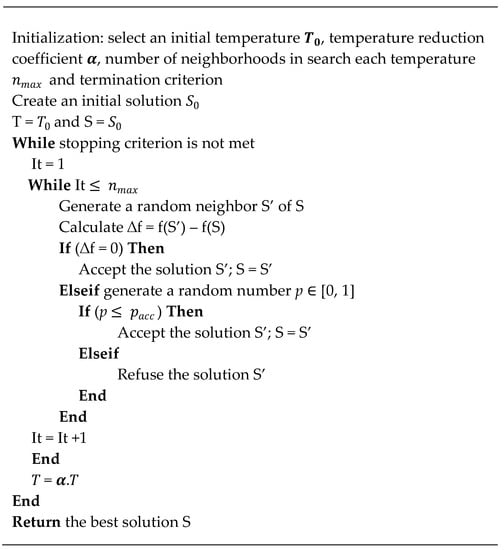
Figure 6.
Pseudocode of the used simulated annealing algorithm.
4.2.3. Particle Swarm Optimization
The PSO, introduced by Eberhart and Kennedy [53], has been applied to solve several real-world engineering problems. This optimization method is based on the collaboration between individuals. It relies on the intelligence of swarms to exploit globally the search space in order to find the optimum or, at the worst case, a best approximate solution in a faster and less expensive way. It is inspired from the interaction and communication between animals (a group of birds, fish, or bees) in search of food [48]. From a population, each particle is viewed as a feasible solution that moves through the problem space to find the best particle and ultimately converges to it. Initial position and velocity are considered for each particle. In each iteration t, the position x and the velocity v of the particles are modified and updated by the following equations:
where Pgb and Pib denote the global best position and the best position found by particle i, respectively. and are randomly chosen parameters in the interval [0, 1] while ∅1 and ∅2 are weights associated to Pib and Pgb, respectively. The pseudocode of the PSO is represented by Figure 7.
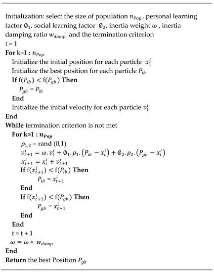
Figure 7.
Pseudocode of the used particle swarm optimization algorithm.
4.2.4. Vibration Damping Optimization
The VDO algorithm is a metaheuristic originally introduced by Mehdizadeh and Tavakkoli-Moghaddam [54]. It is inspired by the SA algorithm and imitates the process of vibration damping in the physics field. There is a practical connection between the vibration damping process and optimization. In the analogy between the vibration damping process and optimization, the states of the oscillation system represent the feasible solutions of the optimization problem. In addition, their energies correspond to the value of the objective function computed at these solutions, while the minimum energy state represents the optimal solution of the problem.
According to the explanation of Mehdizadeh and Tavakkoli-Moghaddam [54], when using a VDO algorithm, a set of principal choices must be made. The algorithm starts with a random choice of an initial solution. Then, its parameters, including the damping coefficient γ, the initial amplitude A1, the standard deviation σ, and the number of neighborhoods at each amplitude nmax, are initialized. In each iteration, a new solution S′ is created by a heuristic perturbation on the current solution S. The neighborhood solution S′ becomes a new solution if the change in an objective function is improved (i.e., in our case, since it is a minimization problem). In the case where this change is not improved, the neighborhood solution becomes a new solution if , which is a random number in the interval [0, 1], is less than or equal to an acceptance probability (represented by (47)). Thus, it is possible to find a global optimal solution from a local optimum. For the high amplitude (at the beginning of the search), there is some flexibility to move from a good solution to a bad one. However, for the lowest amplitude (later in the search), this flexibility decreases. As the procedure proceeds, the amplitude minimizes using (48). The loop is repeated until a stopping criterion is satisfied, as shown in the pseudocode of the VDO algorithm demonstrated in Figure 8.

Figure 8.
Pseudocode of the used vibration damping optimization algorithm.
5. Computational Results
In this section, a case study, including parameter settings of the proposed algorithms and a comparison of the performance and effectiveness of these algorithms, is presented. First, an illustrative example of a French distribution network is presented. The network contains seven suppliers that collaborate to satisfy 13 retailers via shared warehouses and distribution centers. For each set, the maximum number of warehouses and distribution centers to be opened is seven. However, the number of hubs and their storage capacities will be determined by applying the proposed model. The attributed distribution network is shown in Figure 9.
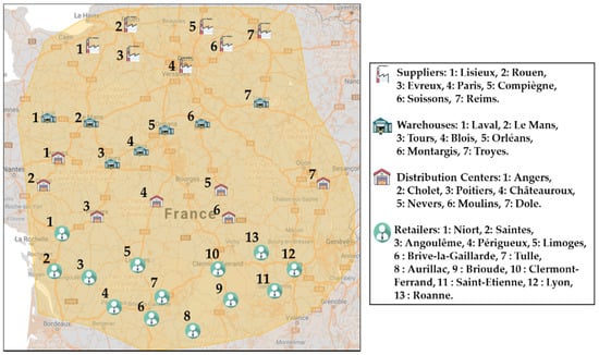
Figure 9.
Used distribution network.
The objective of upstream and downstream collaboration is to consolidate flows by grouping goods, facilitating the transportation of a large amount of freight. For this reason, two types of vehicles (having capacities of 33 and 39 pallets) were used in upstream and downstream parts of the network. As retailers are increasingly demanding in terms of delivery frequency to reduce their stocking levels, a third type of vehicle with a capacity equal to 15 pallets was employed. Therefore, the capacity of the utilized vehicles varies between 15, 33, and 39 pallets. The required data for the used vehicles are represented in Table 2.
Table 2.
The required data for the used vehicles.
The used distances are given in Appendix A using Google Maps. The authorized delivery time for each partner is shown in Table 3.
Table 3.
Level of flexibility in the delivery time of each supplier.
To satisfy the retailer’s demands, we used the same method applied in [35]. In fact, for each product, the retailer demands in each period were randomly selected using uniform distributions in the interval [0, 50] pallets. Some additional data about the used parameters are presented in Table 4. The used data were the same for all scenarios, i.e., they do not vary from one scenario to another.
Table 4.
Other used data.
5.1. Parameters Setting
To ensure an efficient implementation of the proposed algorithms and optimize its performance, its parameters should be well chosen and adequately set. Moreover, the choice of the optimal parameters affects considerably the algorithm exploration. To optimize this choice, several methods can be applied. The classical technique consists in running the proposed algorithms several times with different parameters and keeping the good parameters associated with the best solutions. This method was utilized in the performed experiments since it enables obtaining good results. The different values or levels for all the parameters are shown in Appendix A.
For example, the results of the population size setting , obtained by the genetic algorithm in both scenarios, are given in Appendix A (each algorithm was run five times independently) and their representation is provided in Figure 10. and were set to 0.85 and 0.3, respectively and uniform crossover and Swap mutation were used to determine the best population size that was generated by the levels used in Appendix A (population size between 50 and 300). As demonstrated in Figure 10, the best performance of the genetic algorithm is obtained for a population size of 150 ( = 150).

Figure 10.
Representation of the population size setting for the GA.
Similarly, the best levels for the parameters of all the proposed algorithms (GA, SA, PSO and VDO), helping to achieve the best solutions, were obtained by following the steps explained above. These parameters are shown in Table 5.
Table 5.
The best levels of the parameters of the proposed metaheuristics.
5.2. Numerical Results
In this section, we solve the single objective model (economic or environmental) using the IBM CPLEX 12.10 solver to obtain the exact optimal solution. Due to the variation in solutions given by the algorithms, we computed the average value of the objective function from five runs (e.g., to determine the population number). We used MATLAB software on a computer with an Intel® Core ™ i5-8300HQ CPU (2.30 GHz) with 8 GB of RAM. The results of the Sc1_eco, Sc1_env, Sc2_eco, and Sc2_env scenarios are summarized in Appendix B, respectively. Sc1_eco and Sc2_eco denote, respectively, the first and second solved scenarios with an economic objective function that reduces the logistics costs. On the other hand, Sc1_env and Sc2_env designate, respectively, the first and the second scenarios solved with an environmental objective function reducing CO2 emissions.
The GAP line in the tables represents the relative percentage difference between the approximate solution and the optimal solution. The GAP formula was obtained by the following equation:
where and are, respectively, the objective value obtained by the considered algorithm and the minimum objective value found by using the linear program solved with CPLEX for each scenario. It is obvious that a minimum GAP value is desirable.
The accident risk was calculated with respect to the accident risk caused by a reference distance equal to 2 × 10⁵ km. Therefore, to compute the reference accident risk, the following formula was applied:
To evaluate our study, we compared the performance of the different scenarios, based on several sustainability indicators, and that of the four used algorithms in solving the studied problem.
Based on the results provided by the genetic algorithm shown in Figure 11, we note that the Sc2_eco scenario represented the best scenario from the economic point of view. For example, the total logistics costs for the Sc2_eco scenario and the Sc1_eco scenario werere 14.321 M€ and 14.322 M€, respectively. However, the Sc2_env scenario was the most suitable to protect the environment. It gave better values than Sc1_env for all resolution methods, as shown in Figure 11. For example, the total CO2 emissions obtained with simulated annealing were 3.23 × 10⁹ g CO2 for the Sc2_env scenario against 3.26 × 10⁹ g CO2 for the Sc1_env scenario. From the results of the two scenarios, we can conclude that scenario Sc2 was better than Sc1 because it offers a good compromise between the two economic and environmental objectives.
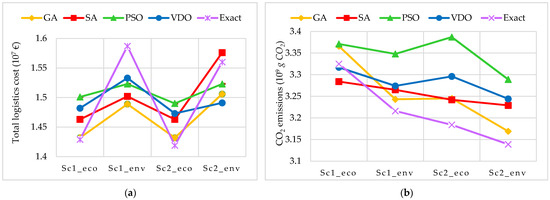
Figure 11.
Results of the different scenarios. (a) Economic results; (b) Environmental results.
The results of the social/societal aspect of sustainability are represented in Figure 12. The distribution of goods via the Sc1_eco scenario generated the lowest accident rate and the lowest fatal accident rate. In addition, the Sc1_env scenario showed the best noise results, compared to the other scenarios. Therefore, from a social/societal point of view, Sc1 scenario is the best.

Figure 12.
Social/Societal results obtained in the different scenarios. (a) Accident risk reduction rate; (b) Noise level.
Based on the findings shown in Figure 13, we noticed that the genetic algorithm could provide the best solutions and even almost the exact optimal values with a GAP lower than 1% for all scenarios. It proved its excellent performance in solving the problem from the economic and environmental point of view. Moreover, comparing all the obtained results, we concluded that the two best metaheuristics were the GA and the SA with average GAP values of 0.73% and 2.47%, respectively, which was valid for most of the economic and environmental scenarios.
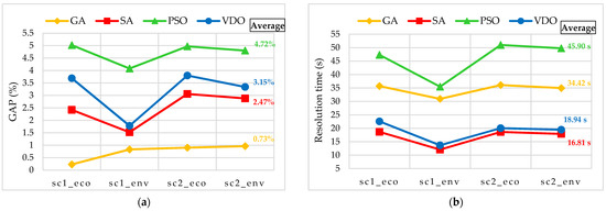
Figure 13.
Performance results of the proposed algorithms. (a) Average GAP values; (b) average execution time values.
Regarding the resolution time, the average required time of GA, SA, PSO, and VDO in seconds were respectively equal to 34.42, 16.81, 45.90, and 18.94, as shown in Figure 13. Moreover, the highest convergence speeds were obtained by the SA and VDO algorithms with a running time of 16.81 s and 18.94 s, respectively. In addition, the average values of the running time show that all the algorithms gave better results compared to those provided by the exact resolution of the linear program (CPLEX), while ensuring a very fast convergence for all scenarios. For example, using CPLEX, the Sc2_eco scenario gave 21,600 s against 36 s obtained when applying the genetic algorithm. Therefore, the total resolution time was reduced by 99.84%. We present the obtained optimal network configurations of the Sc2 scenario using the GA in Figure 14.

Figure 14.
Optimal network configurations of Sc2 scenario using the GA. (a) Sc2_eco; (b) Sc2_env.
6. Sensitivity Analysis
In this section, we study the sensitivity analysis of the performance of the proposed algorithms for the two scenarios in several cases by varying the number of suppliers, warehouses, distribution centers (DCs), retailers, and vehicles. Table 6 shows the ten used instances.
Table 6.
The examined instances.
The results of the linear program solved by the commercial solver CPLEX and the proposed algorithms programmed using MATLAB for both economic and environmental scenarios are shown in Appendix C.
To verify the effectiveness of the introduced algorithms on large instances, we represent the results of Appendix C by the curves in Figure 15 and Figure 16.

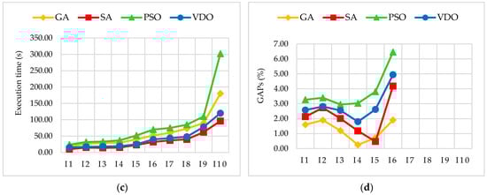
Figure 15.
Comparison between the algorithms used in the different instances of the economic scenarios. (a) Execution time of Sc1_eco; (b) GAPs of Sc2_eco; (c) Execution time of Sc2_eco; (d) GAPs of Sc2_eco.
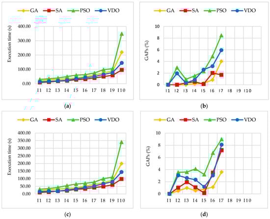
Figure 16.
Comparison of the algorithms used in the different instances of the environmental scenarios. (a) Execution time of Sc1_env; (b) GAPs of Sc2_env; (c) Execution time of Sc2_env; (d) GAPs of Sc2_env.
These curves show that the GA had the best performance with a GAP less than 2%, for the economic scenario, and less than 4% for the environmental one, for all instances. Sometimes, the SA gave better GAPs than all the other algorithms. The example of the I5 instance was considered for the economic and environmental cases of scenario 2 because of the oscillating nature of this algorithm. However, the worst values were obtained by applying the PSO in both economic and environmental scenarios.
Using the curves in Figure 15 and Figure 16, it was obvious that the execution time increased with the rise of the size of the studied instance (i.e., the size of the examined problem). In fact, the SA algorithm was the most efficient in terms of the execution time as it enabled reaching the optimum faster than the other metaheuristics. Therefore, we concluded that the best metaheuristics were the GA and the SA.
The results provided for the different instances were consistent with those of the illustrative example. Indeed, scenario 2 remained the best option, and the proposed metaheuristics gave good solutions with a reasonable execution time.
7. Conclusions
To solve problems caused by the pandemic, the scarcity of natural resources, and the rise in pollution rates, the actors in a logistics system found themselves forced to find an effective solution. In this context, collaboration is the best alternative that may improve the logistics operations and deal with issues related to the different decision levels. In our study, we examined the problem of designing a multiproduct multiperiod, three-echelon distribution network with a heterogeneous fleet of vehicles. This problem belongs to the strategic decision level, which is a critical matter that orients the general orientations of companies.
In this study, we proposed several metaheuristics to solve our model that minimized the logistics costs or CO2 emissions and evaluated the noise level as well as accident rate through the incorporation of two different scenarios. Those metaheuristics were the genetic algorithm, simulated annealing, the particle swarm optimization, and the vibration damping optimization. In addition, to show the performance of our proposed methods, we developed an illustrative example of a distribution network located in France. In order to calibrate the parameters of the introduced metaheuristics, a typical experimental study was carried out. The analysis of the obtained results demonstrated that the genetic algorithm was the best one in terms of GAP in both scenarios. However, when dealing with the computational time, simulated annealing gave the best values within the shortest convergence time.
For future work, it would be interesting to integrate Artificial Intelligence algorithms to improve the results since they enable processing a particularly large amount of data. It is also essential to present other scenarios that take into account the problem of collaborative vehicle routes. Moreover, the consideration of uncertainty in the parameters of problems is very important to imitate reality. Finally, it is necessary to combine the economic objective with the environmental one to select solutions that offer a good compromise between the two objectives. For this reason, we intend to propose a multiobjective simulated annealing (MOSA), a multiobjective particle swarm optimization (MOPSO), and a non-dominated sorting genetic algorithm II (NSGA-II).
Author Contributions
Conceptualization, M.A.G. and N.H.; methodology, M.A.G., N.H., N.M. and L.K.; software, M.A.G.; validation, M.A.G., N.H., N.M. and L.K.; formal analysis, M.A.G.; investigation, M.A.G.; data curation, M.A.G.; writing—original draft preparation, M.A.G.; writing—review and editing, M.A.G., N.H., N.M. and L.K. All authors have read and agreed to the published version of the manuscript.
Funding
This research received no external funding.
Institutional Review Board Statement
Not applicable.
Informed Consent Statement
Not applicable.
Data Availability Statement
Not applicable.
Acknowledgments
The authors would like to thank the anonymous referees from different fields and disciplines for their helpful suggestions.
Conflicts of Interest
The authors declare no conflict of interest.
Appendix A
Table A1.
Distances between suppliers (i) and warehouses (m) in km.
Table A1.
Distances between suppliers (i) and warehouses (m) in km.
| Warehouses | ||||||||
|---|---|---|---|---|---|---|---|---|
| Suppliers | m = 1 | m = 2 | m = 3 | m = 4 | m = 5 | m = 6 | m = 7 | |
| i = 1 | 224 | 282 | 266 | 279 | 358 | 378 | 415 | |
| i = 2 | 152 | 210 | 194 | 206 | 285 | 305 | 342 | |
| i = 3 | 250 | 308 | 265 | 237 | 315 | 336 | 373 | |
| i = 4 | 294 | 264 | 212 | 183 | 262 | 282 | 319 | |
| i = 5 | 232 | 211 | 159 | 131 | 209 | 229 | 266 | |
| i = 6 | 319 | 247 | 209 | 119 | 197 | 217 | 243 | |
| i = 7 | 377 | 307 | 270 | 178 | 243 | 184 | 125 | |
Table A2.
Distances between warehouses (m) and distribution centers (k) in km.
Table A2.
Distances between warehouses (m) and distribution centers (k) in km.
| Distribution Centers | ||||||||
|---|---|---|---|---|---|---|---|---|
| Warehouses | k = 1 | k = 2 | k = 3 | k = 4 | k = 5 | k = 6 | k = 7 | |
| m = 1 | 78 | 143 | 288 | 293 | 410 | 438 | 605 | |
| m = 2 | 95 | 156 | 201 | 206 | 323 | 351 | 531 | |
| m = 3 | 127 | 149 | 106 | 110 | 227 | 255 | 476 | |
| m = 4 | 195 | 217 | 168 | 135 | 182 | 210 | 422 | |
| m = 5 | 247 | 269 | 220 | 146 | 165 | 225 | 369 | |
| m = 6 | 335 | 357 | 308 | 179 | 132 | 192 | 286 | |
| m = 7 | 429 | 490 | 420 | 348 | 260 | 320 | 224 | |
Table A3.
Distances between distribution centers (k) and retailers (j) in km.
Table A3.
Distances between distribution centers (k) and retailers (j) in km.
| Retailers | ||||||||||||||
|---|---|---|---|---|---|---|---|---|---|---|---|---|---|---|
| Distribution centers | j = 1 | j = 2 | j = 3 | j = 4 | j = 5 | j = 6 | j = 7 | j = 8 | j = 9 | j = 10 | j = 11 | j = 12 | j = 13 | |
| m = 1 | 192 | 291 | 322 | 401 | 256 | 351 | 345 | 545 | 507 | 446 | 576 | 595 | 476 | |
| m = 2 | 130 | 229 | 255 | 333 | 246 | 341 | 336 | 568 | 529 | 468 | 598 | 618 | 498 | |
| m = 3 | 77 | 146 | 115 | 194 | 119 | 214 | 208 | 349 | 377 | 316 | 446 | 465 | 346 | |
| m = 4 | 205 | 273 | 223 | 280 | 123 | 213 | 208 | 307 | 269 | 208 | 338 | 357 | 238 | |
| m = 5 | 383 | 451 | 351 | 404 | 251 | 337 | 301 | 282 | 244 | 183 | 243 | 257 | 161 | |
| m = 6 | 411 | 406 | 334 | 342 | 234 | 275 | 238 | 220 | 182 | 121 | 183 | 202 | 101 | |
| m = 7 | 647 | 716 | 554 | 535 | 454 | 469 | 432 | 451 | 413 | 350 | 254 | 195 | 225 | |
Table A4.
Possible levels for the parameters of the proposed algorithms.
Table A4.
Possible levels for the parameters of the proposed algorithms.
| Parameters | Possible Levels |
|---|---|
| 50, 75, 100,150,200, 250, 300 | |
| 0.7, 0.75, 0.8, 0.85, 0.9, 0.95 | |
| 0.1, 0.15, 0.2, 0.25, 0.3 | |
| Crossover | One-point [49], Two-point [60], Uniform [61], Arithmetic [62] |
| Mutation | Swap [63], Displacement [64], Scramble [65], Inversion [66], Insertion [67], Multi non uniform [49], Non uniform [49] |
| Selection | Roulette Wheel, Tournament, Uniform |
| 900, 1000, 1100,1200, 1300, 1400, 1500, 1750, 2000 | |
| ⍺ | 0.93, 0.94, 0.95, 098 |
| 100, 200, 300, 400, 500, 600, 700 | |
| 1.75, 2, 2.25 | |
| 1.75, 2, 2.25 | |
| 0.8, 1, 1.2 | |
| 0.93, 0.94, 0.95, 098 | |
| 0.05, 0.1, 0.15, 0.2, 0.25 | |
| 2, 4, 6, 8, 10, 12, 14, 16, 18, 20 | |
| 1, 1.5, 2, 2.5, 3, 3.5 |
Table A5.
Setting the population size for the applied genetic algorithm.
Table A5.
Setting the population size for the applied genetic algorithm.
| 50 | 75 | 100 | 150 | 200 | 250 | 300 | 500 | |
|---|---|---|---|---|---|---|---|---|
| Total logistics cost in scenario 1 (107 €) | ||||||||
| Execution 1 | 1.4874 | 1.4840 | 1.4466 | 1.4498 | 1.4569 | 1.4535 | 1.4766 | 1.4808 |
| Execution 2 | 1.4846 | 1.4787 | 1.4773 | 1.4556 | 1.4581 | 1.4599 | 1.4731 | 1.4685 |
| Execution 3 | 1.4748 | 1.4578 | 1.4534 | 1.4550 | 1.4548 | 1.4672 | 1.4702 | 1.4756 |
| Execution 4 | 1.4885 | 1.4584 | 1.4694 | 1.4516 | 1.4561 | 1.4787 | 1.4526 | 1.4627 |
| Execution 5 | 1.4846 | 1.4766 | 1.4656 | 1.4567 | 1.4635 | 1.4871 | 1.4786 | 1.4704 |
| Average | 1.4840 | 1.4711 | 1.4624 | 1.4537 | 1.4579 | 1.4693 | 1.4702 | 1.4716 |
| Total logistics cost in scenario 2 (107 €) | ||||||||
| Execution 1 | 1.4413 | 1.4300 | 1.4387 | 1.4368 | 1.4369 | 1.4423 | 1.4374 | 1.4311 |
| Execution 2 | 1.4592 | 1.4713 | 1.4341 | 1.4318 | 1.4328 | 1.4332 | 1.4315 | 1.4339 |
| Execution 3 | 1.4840 | 1.4482 | 1.4305 | 1.4300 | 1.4296 | 1.4309 | 1.4339 | 1.4356 |
| Execution 4 | 1.4377 | 1.4353 | 1.4420 | 1.4315 | 1.4474 | 1.4418 | 1.4417 | 1.4466 |
| Execution 5 | 1.4345 | 1.4601 | 1.4450 | 1.4409 | 1.4329 | 1.4388 | 1.4425 | 1.4405 |
| Average | 1.4513 | 1.4490 | 1.4381 | 1.4342 | 1.4359 | 1.4374 | 1.4374 | 1.4375 |
Appendix B
Table A6.
Results of Sc1 for the different used methods.
Table A6.
Results of Sc1 for the different used methods.
| Indicators | Deterministic Model (CPLEX) | GA | SA | PSO | VDO | ||||||
|---|---|---|---|---|---|---|---|---|---|---|---|
| Eco | Env | Eco | Env | Eco | Env | Eco | Env | Eco | Env | ||
| Economic | Transportation cost (106 €) | 9.2678 | 10.8276 | 9.2799 | 9.9472 | 9.6313 | 10.0434 | 9.9121 | 9.9778 | 9.7843 | 10.3750 |
| Storage cost (103 €) | 6.2650 | 58.3450 | 5.3900 | 6.3700 | 5.6100 | 5.5100 | 5.7000 | 5.9500 | 7.1700 | 4.6700 | |
| Handling cost (105 €) | 1.1341 | 1.1341 | 1.1341 | 1.1341 | 1.1341 | 1.1341 | 1.1341 | 1.1341 | 1.1341 | 1.1341 | |
| Opening cost (106 €) | 4.8445 | 4.8115 | 4.8929 | 4.7908 | 4.8538 | 4.8246 | 4.9444 | 4.9943 | 4.8822 | 4.8084 | |
| Penalty cost (104 €) | 5.6650 | 6.1470 | 2.9880 | 3.1030 | 3.0815 | 3.0270 | 3.0170 | 3.1345 | 2.9120 | 3.1410 | |
| Total logistics cost (107 €) | 1.4289 | 1.5871 | 1.4322 | 1.4889 | 1.4635 | 1.5017 | 1.5006 | 1.5122 | 1.4816 | 1.5333 | |
| Environmental | CO2 emissions due to vehicles (108 g CO2) | 9.0200 | 8.1000 | 9.1800 | 8.4700 | 8.8000 | 8.5200 | 8.6800 | 8.5000 | 8.7600 | 8.6900 |
| CO2 emissions due to hubs (109 g CO2) | 2.4200 | 2.4100 | 2.4400 | 2.3900 | 2.4000 | 2.4100 | 2.4700 | 2.4900 | 2.4400 | 2.4000 | |
| Total CO2 emissions (109 g CO2) | 3.3200 | 3.2100 | 3.3600 | 3.2400 | 3.2800 | 3.2600 | 3.3700 | 3.3400 | 3.3100 | 3.2700 | |
| Social | Accident risk rate (%) | 16.28 | 19.01 | 16.20 | 18.95 | 14.07 | 18.85 | 17.14 | 18.01 | 17.94 | 18.61 |
| Fatal accident rate (%) | 2.44 | 2.85 | 2.43 | 2.84 | 2.11 | 2.83 | 2.57 | 2.70 | 2.69 | 2.79 | |
| Noise level (104 dB) | 2.38 | 1.28 | 2.38 | 1.3 | 1.89 | 1.29 | 1.87 | 1.24 | 1.88 | 1.29 | |
| Execution time (s) | 1820 | 28,800 | 35.71 | 36.09 | 18.66 | 30.93 | 47.34 | 35.47 | 22.57 | 13.68 | |
| GAP (%) | 0.23 | 0.90 | 2.42 | 0.83 | 5.02 | 4.08 | 3.69 | 1.78 | |||
Table A7.
Results of Sc2 for the different used methods.
Table A7.
Results of Sc2 for the different used methods.
| Indicators | Deterministic Model (CPLEX) | GA | SA | PSO | VDO | ||||||
|---|---|---|---|---|---|---|---|---|---|---|---|
| Eco | Env | Eco | Env | Eco | Env | Eco | Env | Eco | Env | ||
| Economic | Transportation cost (106 €) | 9.2093 | 10.5547 | 9.3199 | 10.0713 | 9.6507 | 10.8156 | 9.7274 | 10.1350 | 9.6612 | 9.9193 |
| Storage cost (103 €) | 5.6150 | 71.1000 | 5.4600 | 5.8500 | 5.7000 | 5.9900 | 5.3200 | 6.0900 | 6.5300 | 4.9200 | |
| Handling cost (105 €) | 1.1341 | 1.1341 | 1.1341 | 1.1341 | 1.1341 | 1.1341 | 1.1341 | 1.1341 | 1.1341 | 1.1341 | |
| Opening cost (106 €) | 4.8069 | 4.7977 | 4.8522 | 4.8438 | 4.8269 | 4.7977 | 5.0226 | 4.9452 | 4.9206 | 4.8430 | |
| Penalty cost (104 €) | 5.7770 | 6.2395 | 3.0410 | 3.0440 | 3.0365 | 2.9190 | 2.9440 | 3.1055 | 3.0450 | 3.0635 | |
| Total logistics cost (107 €) | 1.4193 | 1.5599 | 1.4321 | 1.5065 | 1.4627 | 1.5762 | 1.4898 | 1.5231 | 1.4732 | 1.4911 | |
| Environmental | CO2 emissions due to vehicles (108 g CO2) | 7.8000 | 7.4000 | 8.1800 | 7.4700 | 8.2800 | 8.3000 | 8.2600 | 8.1700 | 8.3500 | 8.2200 |
| CO2 emissions due to hubs (109 g CO2) | 2.4000 | 2.4000 | 2.4300 | 2.4200 | 2.4100 | 2.4000 | 2.5600 | 2.4700 | 2.4600 | 2.4200 | |
| Total CO2 emissions (109 g CO2) | 3.1800 | 3.1400 | 3.2400 | 3.1700 | 3.2400 | 3.2300 | 3.3900 | 3.2900 | 3.3000 | 3.2400 | |
| Social | Accident risk rate (%) | 20.03 | 20.08 | 19.88 | 21.70 | 19.75 | 18.44 | 19.84 | 18.80 | 19.75 | 20.38 |
| Fatal accident rate (%) | 3.00 | 3.01 | 2.98 | 3.26 | 2.96 | 2.77 | 2.98 | 2.82 | 2.96 | 3.06 | |
| Noise level (104 dB) | 1.56 | 1.47 | 1.56 | 1.46 | 1.49 | 1.45 | 1.45 | 1.3 | 1.55 | 1.48 | |
| Execution time (s) | 21,600 | 14,400 | 36.09 | 34.97 | 17.91 | 51.02 | 49.78 | 20.05 | 19.47 | ||
| GAP (%) | 0.90 | 0.96 | 2.88 | 4.97 | 4.80 | 3.80 | 3.34 | ||||
Appendix C
Table A8.
Results of the instances in the scenarios obtained by the different resolution methods.
Table A8.
Results of the instances in the scenarios obtained by the different resolution methods.
| Instance | Scenario | Evaluated Indicators | CPLEX | GA | SA | PSO | VDO | |||||
|---|---|---|---|---|---|---|---|---|---|---|---|---|
| Eco | Env | Eco | Env | Eco | Env | Eco | Env | Eco | Env | |||
| I1 | Sc1 | Objective fonction (106 €/109 g CO2) | 8.86 | 2.04 | 8.91 | 2.04 | 8.94 | 2.04 | 8.98 | 2.10 | 8.95 | 2.08 |
| Execution time (s) | 310 | 5200 | 16 | 20.17 | 9.1 | 9.95 | 22.5 | 30.10 | 13.2 | 13.52 | ||
| GAP (%) | 0 | 0 | 0.56 | 0 | 0.90 | 0 | 1.28 | 2.94 | 1 | 1.96 | ||
| Sc2 | Objective fonction (106 €/109 g CO2) | 8.67 | 1.97 | 8.81 | 1.98 | 8.87 | 1.99 | 8.96 | 2.04 | 8.90 | 2.03 | |
| Execution time (s) | 212 | 869 | 18.2 | 21.08 | 10.7 | 10.15 | 24.8 | 31.02 | 15.6 | 15.02 | ||
| GAP (%) | 0 | 0 | 1.6 | 0.50 | 2.13 | 1.01 | 3.27 | 3.55 | 2.58 | 3.04 | ||
| I2 | Sc1 | Objective fonction (107 €/109 g CO2) | 1.36 | 3.18 | 1.37 | 3.18 | 1.39 | 3.19 | 1.4 | 3.21 | 1.4 | 3.19 |
| Execution time (s) | 363 | 2765 | 26.12 | 27.15 | 14.22 | 12.12 | 31.55 | 35.33 | 19.20 | 16.17 | ||
| GAP (%) | 0 | 0 | 0.73 | 0 | 2.46 | 0.31 | 3.00 | 0.94 | 2.78 | 0.31 | ||
| Sc2 | Objective fonction (107 €/109 g CO2) | 1.32 | 3.05 | 1.35 | 3.08 | 1.36 | 3.11 | 1.37 | 3.16 | 1.36 | 3.13 | |
| Execution time (s) | 240 | 693 | 27.45 | 28.19 | 15.9 | 13.45 | 31.88 | 36.11 | 17.80 | 18.07 | ||
| GAP (%) | 0 | 0 | 1.9 | 0.98 | 2.73 | 1.96 | 3.40 | 3.60 | 2.81 | 2.62 | ||
| I3 | Sc1 | Objective fonction (107 €/109 g CO2) | 2.61 | 5.87 | 2.63 | 5.88 | 2.64 | 5.90 | 2.69 | 5.96 | 2.65 | 5.92 |
| Execution time (s) | 901 | 9256 | 29.54 | 30.30 | 15.54 | 18.17 | 32.01 | 40.78 | 18.40 | 20.00 | ||
| GAP (%) | 0 | 0 | 0.74 | 0.17 | 1.26 | 0.51 | 3.05 | 1.53 | 1.52 | 0.85 | ||
| Sc2 | Objective fonction (107 €/109 g CO2) | 2.55 | 5.57 | 2.58 | 5.60 | 2.6 | 5.63 | 2.63 | 5.80 | 2.62 | 5.70 | |
| Execution time (s) | 1432 | 5899 | 30.03 | 32.31 | 14.95 | 19.22 | 33.22 | 43.44 | 17.95 | 18.92 | ||
| GAP (%) | 0 | 0 | 1.20 | 0.53 | 2.01 | 1.07 | 2.95 | 4.12 | 2.55 | 2.33 | ||
| I4 | Sc1 | Objective fonction (107 €/109 g CO2) | 3.30 | 7.33 | 3.32 | 7.35 | 3.38 | 7.34 | 3.4 | 7.50 | 3.39 | 7.52 |
| Execution time (s) | 10,852 | 10,952 | 30.57 | 34.55 | 15.09 | 21.00 | 33.66 | 50.22 | 17.08 | 24.88 | ||
| GAP (%) | 0 | 0 | 0.62 | 0.27 | 2.58 | 0.13 | 2.95 | 2.31 | 2.64 | 2.59 | ||
| Sc2 | Objective fonction (107 €/109 g CO2) | 3.24 | 6.89 | 3.25 | 6.95 | 3.28 | 6.90 | 3.34 | 7.11 | 3.3 | 6.97 | |
| Execution time (s) | 2252 | 4796 | 29.95 | 36.45 | 15.52 | 22.88 | 37.01 | 55.54 | 19.02 | 26.46 | ||
| GAP (%) | 0 | 0 | 0.25 | 0.78 | 1.18 | 0.14 | 3.03 | 3.20 | 1.80 | 1.16 | ||
| I5 | Sc1 | Objective fonction (107 €/109 g CO2) | 4.27 | 9.40 | 4.35 | 9.48 | 4.33 | 9.59 | 4.42 | 9.85 | 4.3 | 9.70 |
| Execution time (s) | 12,198 | 17,555 | 38.09 | 40.08 | 20.01 | 28.12 | 45.66 | 60.86 | 22.32 | 35.49 | ||
| GAP (%) | 0 | 0 | 1.87 | 0.84 | 1.52 | 2.02 | 3.52 | 4.88 | 2.34 | 3.19 | ||
| Sc2 | Objective fonction (107 €/109 g CO2) | 4.19 | 8.88 | 4.22 | 8.98 | 4.21 | 9.19 | 4.35 | 9.48 | 4.3 | 9.15 | |
| Execution time (s) | 5296 | 9998 | 39.95 | 39.85 | 23.22 | 30.09 | 52.02 | 65.42 | 25.66 | 33.32 | ||
| GAP (%) | 0 | 0 | 0.71 | 1.12 | 0.47 | 3.50 | 3.81 | 6.75 | 2.62 | 3.04 | ||
| I6 | Sc1 | Objective fonction (107 €/109 g CO2) | 5.36 | 1.18 | 5.49 | 1.23 | 5.50 | 1.20 | 5.64 | 1.28 | 5.57 | 1.25 |
| Execution time (s) | 25,999 | 15,033 | 50.23 | 49.46 | 29.52 | 32.25 | 65.55 | 63.58 | 35.77 | 42.15 | ||
| GAP (%) | 0 | 0 | 2.42 | 4.02 | 2.61 | 1.70 | 5.19 | 8.47 | 4.01 | 5.93 | ||
| Sc2 | Objective fonction (107 €/109 g CO2) | 5.26 | 1.11 | 5.36 | 1.15 | 5.48 | 1.19 | 5.60 | 1.21 | 5.52 | 1.20 | |
| Execution time (s) | 21,265 | 10,005 | 52.25 | 52.55 | 32.89 | 34.55 | 70.05 | 70.19 | 40.01 | 43.16 | ||
| GAP (%) | 0 | 0 | 1.91 | 3.60 | 4.18 | 7.20 | 6.46 | 9.00 | 4.94 | 8.10 | ||
| I7 | Sc1 | Objective fonction (107 €/109 g CO2) | NF 1 | NF 1 | 6.69 | 1.28 | 6.73 | 1.29 | 6.78 | 1.30 | 6.76 | 1.32 |
| Execution time (s) | NF 1 | NF 1 | 59.72 | 60.25 | 38.45 | 40.56 | 77.22 | 75.57 | 45.63 | 50.56 | ||
| GAP (%) | NF 1 | NF 1 | - | - | - | - | - | - | - | - | ||
| Sc2 | Objective fonction (107 €/109 g CO2) | NF 1 | NF 1 | 6.52 | 1.20 | 6.59 | 1.22 | 6.69 | 1.25 | 6.63 | 1.30 | |
| Execution time (s) | NF 1 | NF 1 | 60.12 | 62.66 | 37.51 | 42.57 | 75.07 | 78.98 | 44.44 | 52.55 | ||
| GAP (%) | NF 1 | NF 1 | - | - | - | - | - | - | - | - | ||
| I8 | Sc1 | Objective fonction (107 €/109 g CO2) | NF 1 | NF 1 | 7.18 | 1.33 | 7.24 | 1.48 | 7.36 | 1.59 | 5.32 | 1.60 |
| Execution time (s) | NF 1 | NF 1 | 75.35 | 76.68 | 42.23 | 50.65 | 90.01 | 98.12 | 50.08 | 65.89 | ||
| GAP (%) | NF 1 | NF 1 | - | - | - | - | - | - | - | - | ||
| Sc2 | Objective fonction (107 €/109 g CO2) | NF 1 | NF 1 | 7.09 | 1.25 | 7.22 | 1.27 | 7.35 | 1.36 | 5.30 | 1.48 | |
| Execution time (s) | NF 1 | NF 1 | 73.86 | 74.89 | 40.18 | 49.98 | 85.52 | 100.01 | 47.98 | 67.89 | ||
| GAP (%) | NF 1 | NF 1 | - | - | - | - | - | - | - | - | ||
| I9 | Sc1 | Objective fonction (107 €/109 g CO2) | NF 1 | NF 1 | 7.72 | 1.58 | 7.78 | 1.64 | 7.82 | 1.68 | 7.80 | 1.66 |
| Execution time (s) | NF 1 | NF 1 | 90.17 | 88.88 | 60.16 | 59.52 | 102.15 | 105.55 | 75.45 | 78.89 | ||
| GAP (%) | NF 1 | NF 1 | - | - | - | - | - | - | - | - | ||
| Sc2 | Objective fonction (107 €/109 g CO2) | NF 1 | NF 1 | 7.09 | 1.38 | 7.09 | 1.47 | 7.09 | 1.39 | 7.09 | 1.55 | |
| Execution time (s) | NF 1 | NF 1 | 89.89 | 90.36 | 61.73 | 60.66 | 110.14 | 111.12 | 77.76 | 80.15 | ||
| GAP (%) | NF 1 | NF 1 | - | - | - | - | - | - | - | - | ||
| I10 | Sc1 | Objective fonction (108 €/109 g CO2) | NF 1 | NF 1 | 1.10 | 2.38 | 1.15 | 2.42 | 1.18 | 2.68 | 1.16 | 2.52 |
| Execution time (s) | NF 1 | NF 1 | 240.69 | 220.00 | 95.23 | 96.33 | 389.91 | 349.98 | 130.25 | 145.46 | ||
| GAP (%) | NF 1 | NF 1 | - | - | - | - | - | - | - | - | ||
| Sc2 | Objective fonction (108 €/109 g CO2) | NF 1 | NF 1 | 1.02 | 2.12 | 1.09 | 2.22 | 1.15 | 2.57 | 1.12 | 2.51 | |
| Execution time (s) | NF 1 | NF 1 | 180.45 | 200.12 | 96.59 | 98.87 | 302.12 | 341.45 | 120.88 | 144.42 | ||
| GAP (%) | NF 1 | NF 1 | - | - | - | - | - | - | - | - | ||
1 Not Found.
References
- Commissariat Général au Développement Durable. Chiffres Clés du Transport, 2021 ed.; Commissariat Général au Développement Durable: Paris, France, 2021. [Google Scholar]
- Camarinha-Matos, L.M. Collaborative Networks: A Mechanism for Enterprise Agility and Resilience. In Enterprise Interoperability VI; Mertins, K., Bénaben, F., Poler, R., Bourrières, J.-P., Eds.; Springer International Publishing: Cham, Switzerland, 2014; pp. 3–11. ISBN 978-3-319-04947-2. [Google Scholar]
- Aloui, A.; Hamani, N.; Derrouiche, R.; Delahoche, L. Systematic Literature Review on Collaborative Sustainable Transportation: Overview, Analysis and Perspectives. Transp. Res. Interdiscip. Perspect. 2020, 9, 100291. [Google Scholar] [CrossRef]
- Koulougli, K. Combinaison de la Collaboration Horizontale et Verticale pour l’Optimisation de la Chaîne d’Approvisionnement Internationale. Master’s Thesis, École de Technologie Supérieure, Montréal, QC, Canada, 2015. [Google Scholar]
- Snoussi, I.; Hamani, N.; Mrabti, N.; Kermad, L. Robust Optimization for Collaborative Distribution Network Design Problem. In Smart and Sustainable Collaborative Networks 4.0, IFIP AICT Advances in Information and Communication Technology; Springer: Cham, Switzerland, 2021; Volume 629. [Google Scholar]
- Mrabti, N.; Gargouri, M.A.; Hamani, N.; Kermad, L. Towards a sustainable collaborative distribution network 4.0 with blockchain involvement. In Smart and Sustainable Collaborative Networks 4.0, IFIP AICT Advances in Information and Communication Technology; Springer: Cham, Switzerland, 2021; Volume 629. [Google Scholar]
- Snoussi, I.; Hamani, N.; Mrabti, N.; Kermad, L. A Robust Mixed-Integer Linear Programming Model for Sustainable Collaborative Distribution. Mathematics 2021, 9, 2318. [Google Scholar] [CrossRef]
- Pan, S.; Trentesaux, D.; Ballot, E.; Huang, G.Q. Horizontal Collaborative Transport: Survey of Solutions and Practical Implementation Issues. Int. J. Prod. Res. 2019, 57, 5340–5361. [Google Scholar] [CrossRef] [Green Version]
- Amer, L.E.; Eltawil, A.B. Analysis of Quantitative Models of Horizontal Collaboration in Supply Chain Network Design: Towards “Green Collaborative” Strategies. In Proceedings of the 2015 International Conference on Industrial Engineering and Operations Management (IEOM), Dubai, United Arab Emirates, 3–5 March 2015; pp. 1–10. [Google Scholar]
- Misni, F.; Lee, L.S. A Review on Strategic, Tactical and Operational Decision Planning in Reverse Logistics of Green Supply Chain Network Design. J. Comput. Commun. 2017, 5, 83–104. [Google Scholar] [CrossRef] [Green Version]
- Moutaoukil, A.; Derrouiche, R.; Neubert, G. Pooling Supply Chain: Literature Review of Collaborative Strategies. In Proceedings of the Collaborative Networks in the Internet of Services; Camarinha-Matos, L.M., Xu, L., Afsarmanesh, H., Eds.; Springer: Berlin/Heidelberg, Germany, 2012; pp. 513–525. [Google Scholar]
- Cuda, R.; Guastaroba, G.; Speranza, M.G. A Survey on Two-Echelon Routing Problems. Comput. Oper. Res. 2015, 55, 185–199. [Google Scholar] [CrossRef]
- Muñoz-Villamizar, A.; Montoya-Torres, J.R.; Faulin, J. Impact of the Use of Electric Vehicles in Collaborative Urban Transport Networks: A Case Study. Transp. Res. Part Transp. Environ. 2017, 50, 40–54. [Google Scholar] [CrossRef]
- Hu, L.; Zhu, J.X.; Wang, Y.; Lee, L.H. Joint Design of Fleet Size, Hub Locations, and Hub Capacities for Third-Party Logistics Networks with Road Congestion Constraints. Transp. Res. Part E Logist. Transp. Rev. 2018, 118, 568–588. [Google Scholar] [CrossRef]
- Campbell, J.F.; O’Kelly, M.E. Twenty-Five Years of Hub Location Research. Transp. Sci. 2012, 46, 153–169. [Google Scholar] [CrossRef]
- O’Kelly, M.E. The Location of Interacting Hub Facilities. Transp. Sci. 1986, 20, 92–106. [Google Scholar] [CrossRef]
- O’Kelly, M.E. A Quadratic Integer Program for the Location of Interacting Hub Facilities. Eur. J. Oper. Res. 1987, 32, 393–404. [Google Scholar] [CrossRef]
- Contreras, I.; Fernández, E.; Reinelt, G. Minimizing the Maximum Travel Time in a Combined Model of Facility Location and Network Design. Omega 2012, 40, 847–860. [Google Scholar] [CrossRef]
- Corberán, A.; Peiró, J.; Laguna, M.; Marti, R. Models and Solution Methods for the Uncapacitated R-Allocation p-Hub Equitable Center Problem. Int. Trans. Oper. Res. 2017, 25. [Google Scholar] [CrossRef]
- Contreras, I.; O’Kelly, M. Hub Location Problems. In Location Science; Laporte, G., Nickel, S., Saldanha da Gama, F., Eds.; Springer International Publishing: Cham, Switzerland, 2019; pp. 327–363. ISBN 978-3-030-32177-2. [Google Scholar]
- Alumur, S.A.; Campbell, J.F.; Contreras, I.; Kara, B.Y.; Marianov, V.; O’Kelly, M.E. Perspectives on Modeling Hub Location Problems. Eur. J. Oper. Res. 2021, 291, 1–17. [Google Scholar] [CrossRef]
- Farahani, R.Z.; Hekmatfar, M.; Arabani, A.B.; Nikbakhsh, E. Hub Location Problems: A Review of Models, Classification, Solution Techniques, and Applications. Comput. Ind. Eng. 2013, 64, 1096–1109. [Google Scholar] [CrossRef]
- Contreras, I. Hub Location Problems. In Location Science; Springer: Berlin/Heidelberg, Germany, 2015; pp. 311–344. [Google Scholar]
- Rodríguez, V.; Alvarez, M.J.; Barcos, L. Hub Location under Capacity Constraints. Transp. Res. Part E Logist. Transp. Rev. 2007, 43, 495–505. [Google Scholar] [CrossRef]
- Kratica, J.; Stanimirović, Z.; Tošić, D.; Filipović, V. Two Genetic Algorithms for Solving the Uncapacitated Single Allocation P-Hub Median Problem. Eur. J. Oper. Res. 2007, 182, 15–28. [Google Scholar] [CrossRef]
- Randall, M. Solution Approaches for the Capacitated Single Allocation Hub Location Problem Using Ant Colony Optimisation. Inf. Technol. Pap. 2008, 39, 239–261. [Google Scholar] [CrossRef]
- Ilić, A.; Urošević, D.; Brimberg, J.; Mladenović, N. A General Variable Neighborhood Search for Solving the Uncapacitated Single Allocation P-Hub Median Problem. Eur. J. Oper. Res. 2010, 206, 289–300. [Google Scholar] [CrossRef]
- Stanimirović, Z. A Genetic Algorithm Approach for the Capacitated Single Allocation P-Hub Median Problem. Comput. Inform. 2010, 29, 117–132. [Google Scholar]
- Lin, C.-C.; Lin, J.-Y.; Chen, Y.-C. The Capacitated P-Hub Median Problem with Integral Constraints: An Application to a Chinese Air Cargo Network. Appl. Math. Model. 2012, 36, 2777–2787. [Google Scholar] [CrossRef]
- Yang, K.; Liu, Y.-K.; Yang, G.-Q. Solving Fuzzy P-Hub Center Problem by Genetic Algorithm Incorporating Local Search. Appl. Soft Comput. 2013, 13, 2624–2632. [Google Scholar] [CrossRef]
- Yang, K.; Liu, Y.; Yang, G. An Improved Hybrid Particle Swarm Optimization Algorithm for Fuzzy P-Hub Center Problem. Comput. Ind. Eng. 2013, 64, 133–142. [Google Scholar] [CrossRef]
- Ghaderi, A.; Rahmaniani, R. Meta-Heuristic Solution Approaches for Robust Single Allocation p-Hub Median Problem with Stochastic Demands and Travel Times. Int. J. Adv. Manuf. Technol. 2015, 82, 1627–1647. [Google Scholar] [CrossRef]
- Fazel Zarandi, M.H.; Davari, S.; Haddad Sisakht, A. An Empirical Comparison of Simulated Annealing and Iterated Local Search for the Hierarchical Single Allocation Hub Median Location Problem. Sci. Iran. 2015, 22, 1203–1217. [Google Scholar]
- Damgacioglu, H.; Dinler, D.; Evin Ozdemirel, N.; Iyigun, C. A Genetic Algorithm for the Uncapacitated Single Allocation Planar Hub Location Problem. Comput. Oper. Res. 2015, 62, 224–236. [Google Scholar] [CrossRef]
- Serper, E.Z.; Alumur, S.A. The Design of Capacitated Intermodal Hub Networks with Different Vehicle Types. Transp. Res. Part B Methodol. 2016, 86, 51–65. [Google Scholar] [CrossRef]
- Rabbani, M.; Farrokhi-Asl, H.; Heidari, R. Genetic Algorithm-Based Optimization Approach for an Uncapacitated Single Allocation P-Hub Center Problem with More Realistic Cost Structure. J. Ind. Syst. Eng. 2017, 10, 108–124. [Google Scholar]
- Mirabi, M.; Seddighi, P. Hybrid Ant Colony Optimization for Capacitated Multiple-Allocation Cluster Hub Location Problem. Artif. Intell. Eng. Des. Anal. Manuf. 2017, 32, 44–58. [Google Scholar] [CrossRef]
- Monemi, R.N.; Gelareh, S.; Hanafi, S.; Maculan, N. A Co-Opetitive Framework for the Hub Location Problems in Transportation Networks. Optimization 2017, 66, 2089–2106. [Google Scholar] [CrossRef]
- Ghaffarinasab, N.; Motallebzadeh, A.; Jabarzadeh, Y.; Kara, B.Y. Efficient Simulated Annealing Based Solution Approaches to the Competitive Single and Multiple Allocation Hub Location Problems. Comput. Oper. Res. 2018, 90, 173–192. [Google Scholar] [CrossRef]
- Bashiri, M.; Rezanezhad, M.; Tavakkoli-Moghaddam, R.; Hasanzadeh, H. Mathematical Modeling for a P-Mobile Hub Location Problem in a Dynamic Environment by a Genetic Algorithm. Appl. Math. Model. 2018, 54, 151–169. [Google Scholar] [CrossRef]
- Lüer-Villagra, A.; Eiselt, H.A.; Marianov, V. A Single Allocation P-Hub Median Problem with General Piecewise-Linear Costs in Arcs. Comput. Ind. Eng. 2019, 128, 477–491. [Google Scholar] [CrossRef]
- Özgün-Kibiroğlu, Ç.; Serarslan, M.N.; Topcu, Y.İ. Particle Swarm Optimization for Uncapacitated Multiple Allocation Hub Location Problem under Congestion. Expert Syst. Appl. 2019, 119, 1–19. [Google Scholar] [CrossRef]
- Shang, X.; Yang, K.; Wang, W.; Wang, W.; Zhang, H.; Celic, S. Stochastic Hierarchical Multimodal Hub Location Problem for Cargo Delivery Systems: Formulation and Algorithm. IEEE Access 2020, 8, 55076–55090. [Google Scholar] [CrossRef]
- Shang, X.; Yang, K.; Jia, B.; Gao, Z. Distributionally Robust Cluster-Based Hierarchical Hub Location Problem for the Integration of Urban and Rural Public Transport System. Comput. Ind. Eng. 2021, 155, 107181. [Google Scholar] [CrossRef]
- Wang, M.; Cheng, Q.; Huang, J.; Cheng, G. Research on Optimal Hub Location of Agricultural Product Transportation Network Based on Hierarchical Hub-and-Spoke Network Model. Phys. Stat. Mech. Appl. 2021, 566, 125412. [Google Scholar] [CrossRef]
- Mrabti, N.; Hamani, N.; Delahoche, L. The Pooling of Sustainable Freight Transport. J. Oper. Res. Soc. 2020, 1–16. [Google Scholar] [CrossRef]
- Abbassi, A.; Alaoui, A.; Boukachour, J. Modelling and Solving a Bi-Objective Intermodal Transport Problem of Agricultural Products. Int. J. Ind. Eng. Comput. 2018, 9, 439–460. [Google Scholar] [CrossRef]
- Shoja, A.; Molla-Alizadeh-Zavardehi, S.; Niroomand, S. Adaptive Meta-Heuristic Algorithms for Flexible Supply Chain Network Design Problem with Different Delivery Modes. Comput. Ind. Eng. 2019, 138, 106107. [Google Scholar] [CrossRef]
- Holland, J.H. Adaptation in Natural and Artificial Systems; MIT Press: Cambridge, MA, USA, 1975. [Google Scholar]
- Goodarzian, F.; Kumar, V.; Abraham, A. Hybrid Meta-Heuristic Algorithms for a Supply Chain Network Considering Different Carbon Emission Regulations Using Big Data Characteristics. Soft Comput. 2021, 25, 7527–7557. [Google Scholar] [CrossRef]
- Altiparmak, F.; Gen, M.; Lin, L.; Paksoy, T. A Genetic Algorithm Approach for Multi-Objective Optimization of Supply Chain Networks. Comput. Ind. Eng. 2006, 51, 196–215. [Google Scholar] [CrossRef]
- Kirkpatrick, S.; Gelatt, C.D.; Vecchi, M.P. Optimization by Simulated Annealing. Science 1983, 220, 671–680. [Google Scholar] [CrossRef]
- Eberhart, R.; Kennedy, J. A New Optimizer Using Particle Swarm Theory. In Proceedings of the MHS’95, the Sixth International Symposium on Micro Machine and Human Science, Nagoya, Japan, 4–6 October 1995; pp. 39–43. [Google Scholar]
- Mehdizadeh, E.; Tavakkoli-Moghaddam, R. Vibration Damping Optimization. In Proceedings of the International Conference of Operations Research and Global Business, City, Germany, 3–5 September 2008. [Google Scholar]
- Mrabti, N.; Hamani, N.; Delahoche, L. A sustainable collaborative approach to the distribution network design problem with CO2 emissions allocation. Int. J. Shipp. Transp. Logist. 2021, 13, 1. [Google Scholar] [CrossRef]
- Hickman, J.; Hassel, D.; Joumard, R.; Samaras, Z.; Sorenson, S. Methodology for Calculating Transport Emissions and Energy Consumption; The National Academies of Sciences, Engineering, Medicine: Washington, DC, USA, 1999. [Google Scholar]
- Observatory Energy Environment of Transport (OEET). Available online: https://www.bilans-ges.ademe.fr/documentation/UPLOAD_DOC_FR/index.htm?transport_routier_de_marchandi%20.html (accessed on 3 April 2021).
- Ayadi, A. Vers Une Organisation Globale Durable de l’approvisionnement des Ménages: Bilans Économiques et Environnementaux de Différentes Chaînes de Distribution Classiques et Émergentes Depuis l’Entrepôt Du Fournisseur Jusqu’au Domicile Du Ménage. Ph.D. Thesis, University of Lyon, Lyon, France, 2014. [Google Scholar]
- Agence De l’Environnement et de la Maîtrise de l’Energie (ADEME). Calcul des Facteurs d’émissions et Sources Bibliographiques Utilisées. Méthode Bilan Carbone; Agence De l’Environnement et de la Maîtrise de l’Energie: Besançon, France, 2010. [Google Scholar]
- De Jong, K.A. An Analysis of the Behavior of a Class of Genetic Adaptive Systems. Ph.D. Thesis, University of Michigan, Ann Arbor, MI, USA, 1975. [Google Scholar]
- Syswerda, G. Uniform Crossover in Genetic Algorithms. In Proceedings of the Third International Conference on Genetic Algorithms, Fairfax, VA, USA, 4–7 June 1989; pp. 2–9. [Google Scholar]
- Michalewicz, Z.; Schoenauer, M. Evolutionary Algorithms for Constrained Parameter Optimization Problems. Evol. Comput. 1996, 4, 1–32. [Google Scholar] [CrossRef]
- Larrañaga, P.; Kuijpers, C.M.H.; Murga, R.H.; Inza, I.; Dizdarevic, S. Genetic Algorithms for the Travelling Salesman Problem: A Review of Representations and Operators. Artif. Intell. Rev. 1999, 13, 129–170. [Google Scholar] [CrossRef]
- Michalewicz, Z. Genetic Algorithms + Data Structures = Evolution Programs, 3rd ed.; Springer-Verlag: Berlin/Heidelberg, Germany, 1996; ISBN 978-3-540-60676-5. [Google Scholar]
- Syswerda, G. Scheduling Optimization Using Genetic Algorithms. Handb. Genet. Algorithms. 1991. Available online: https://ci.nii.ac.jp/naid/10021131794/ (accessed on 30 October 2021).
- Fogel, D.B. A Parallel Processing Approach to a Multiple Travelling Salesman Problem Using Evolutionary Programming. In Proceedings of the Fourth Annual Symposium on Parallel Processing, Fullerton, CA, USA; 1990; pp. 318–326. Available online: https://scholar.google.com.hk/scholar?hl=en&as_sdt=0%2C5&q=Fogel%2C+D.B.+A+Parallel+Processing+Approach+to+a+Multiple+Travelling+Salesman+Problem+Using+Evolutionary+Programming.+In+Proceedings+of+the+Fourth+Annual+Symposium+on+Parallel+Processing%2C+Fullerton%2C+CA%2C+USA&btnG= (accessed on 30 October 2021).
- Fogel, D.B. An Evolutionary Approach to the Traveling Salesman Problem. Biol. Cybern. 1988, 60, 139–144. [Google Scholar] [CrossRef]
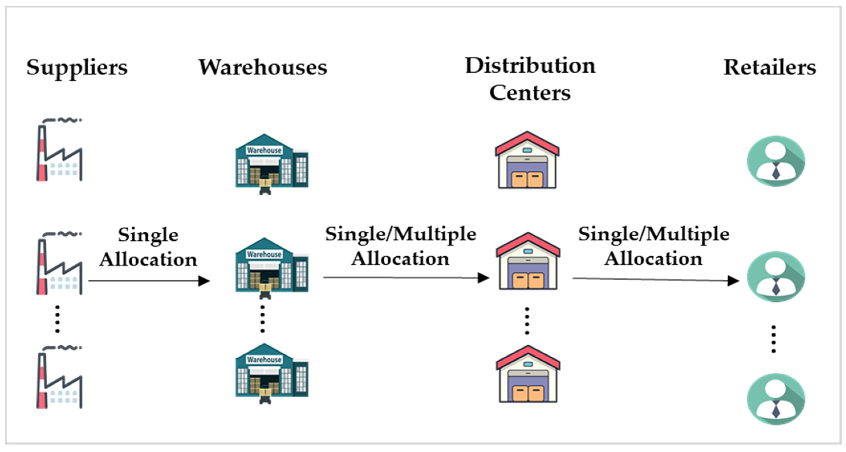
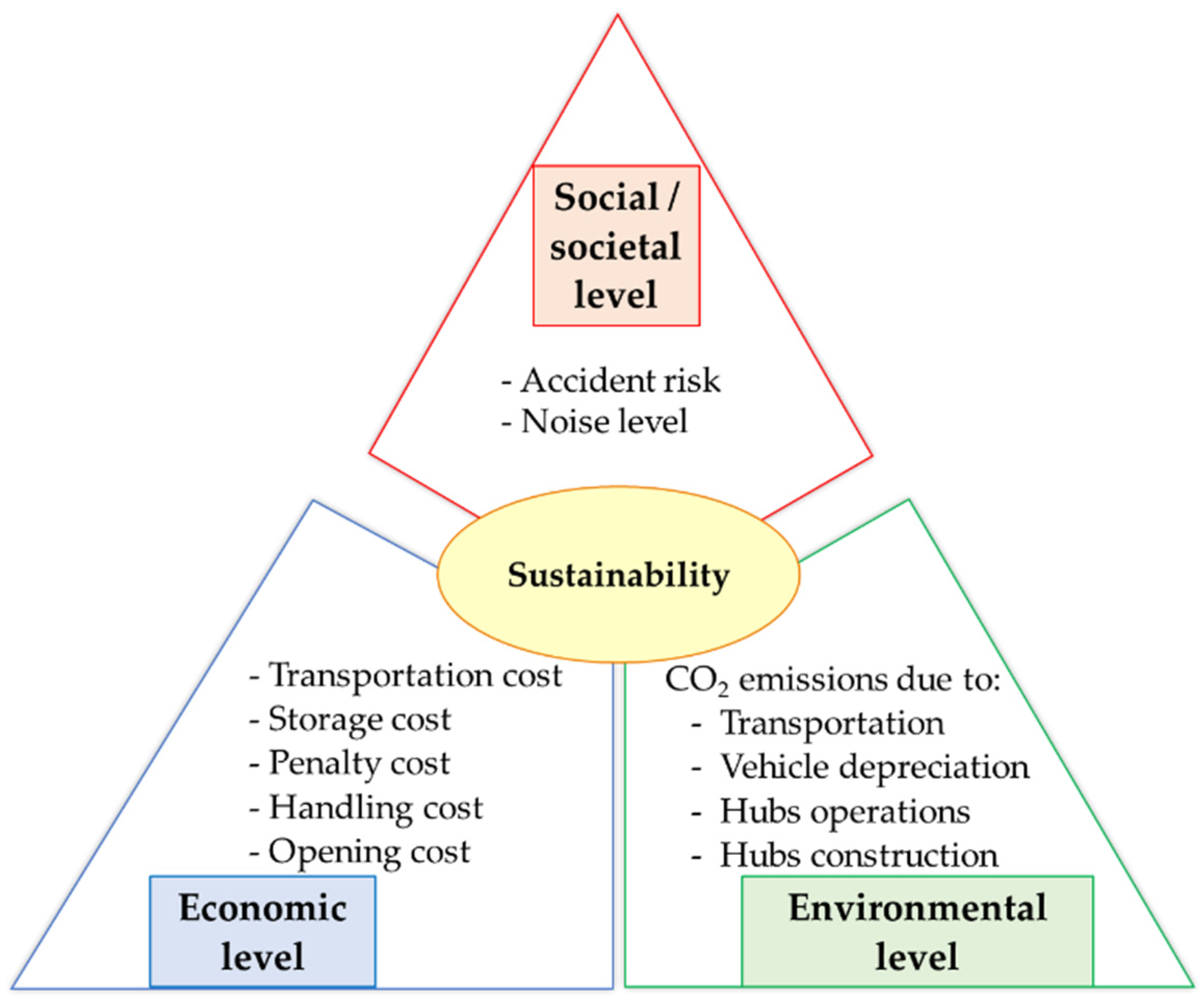
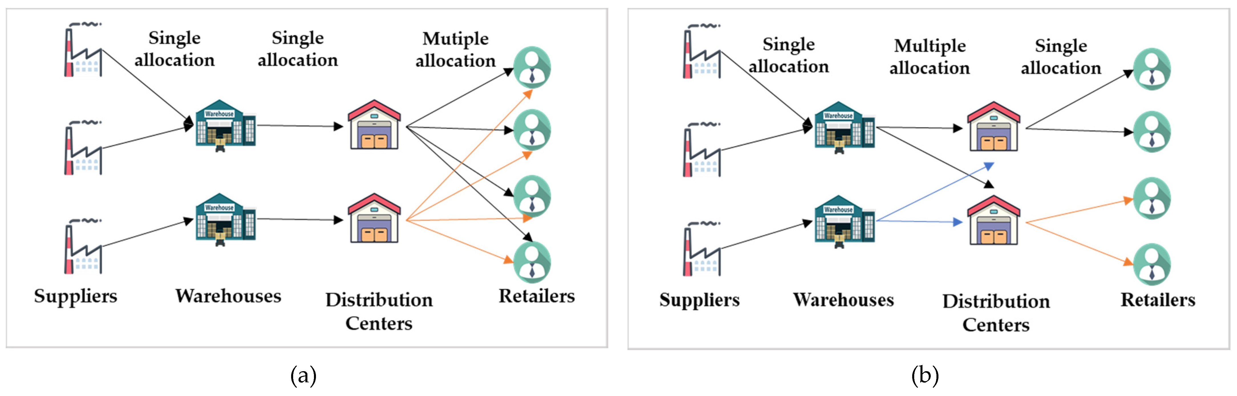
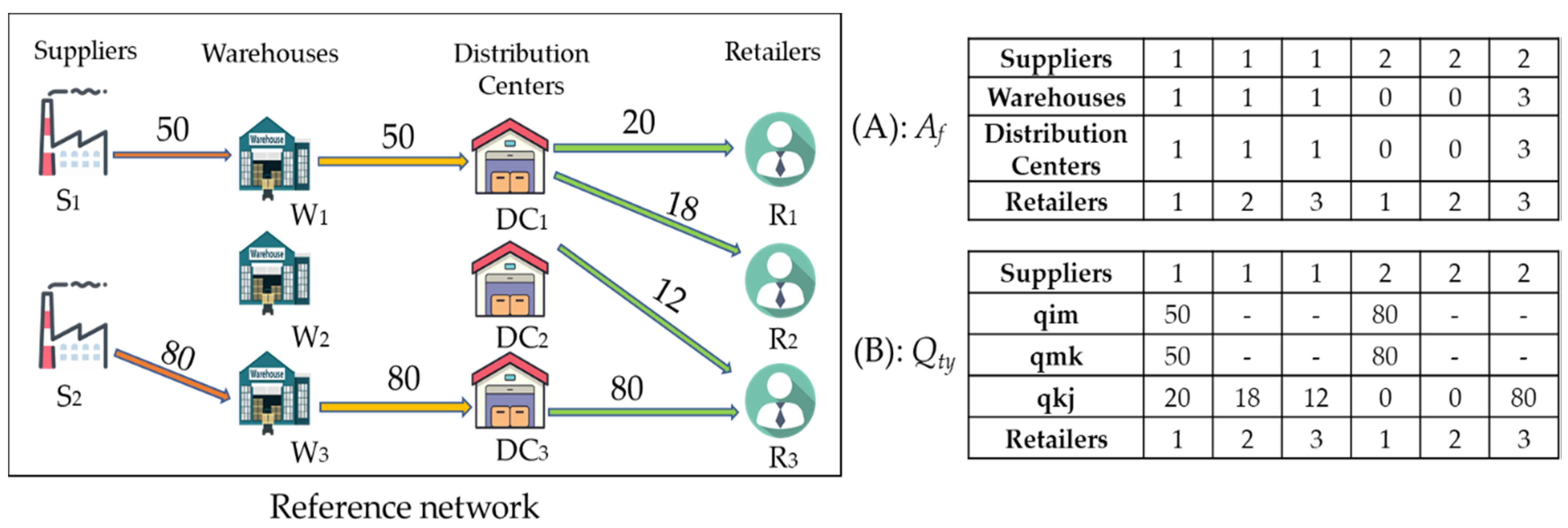

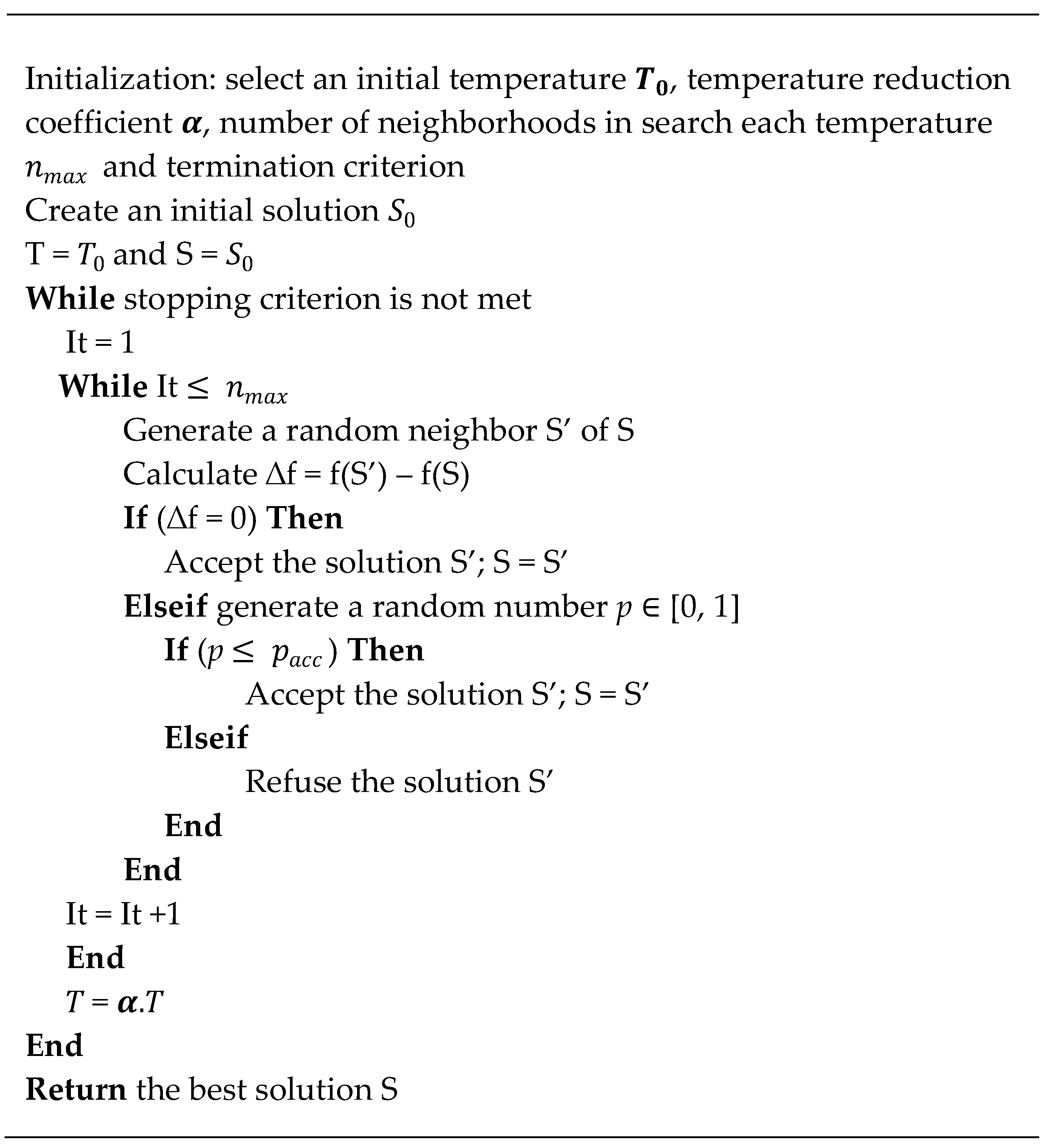
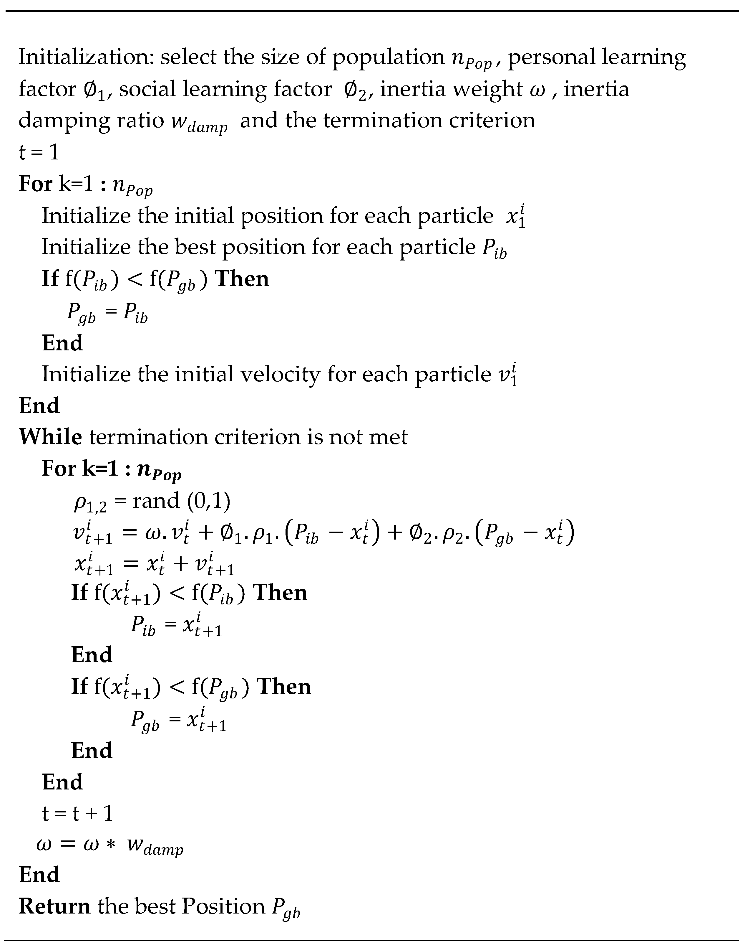
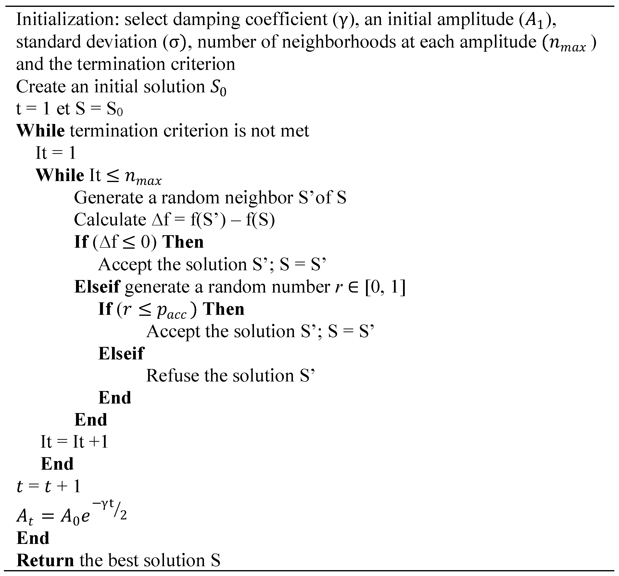

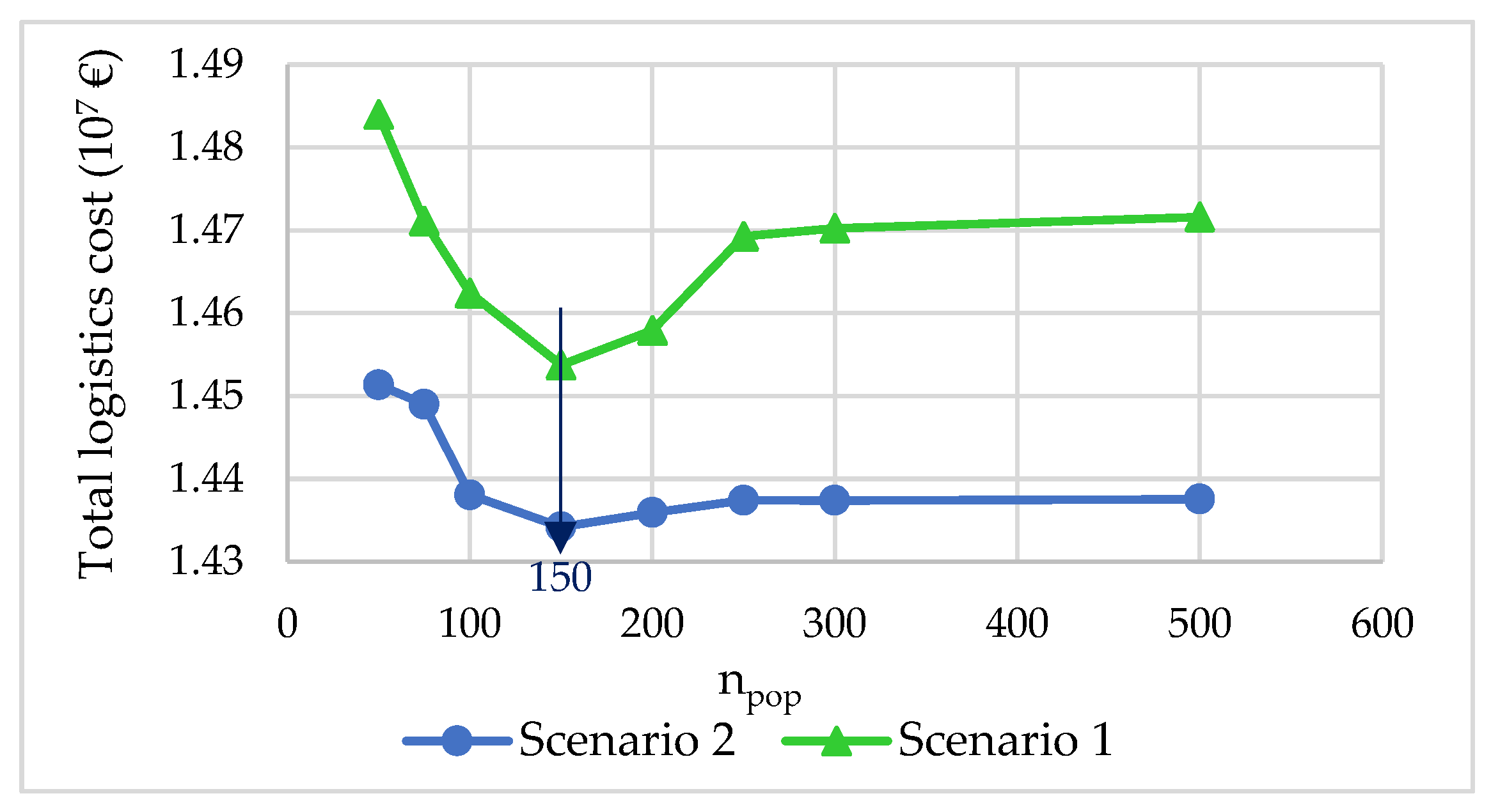

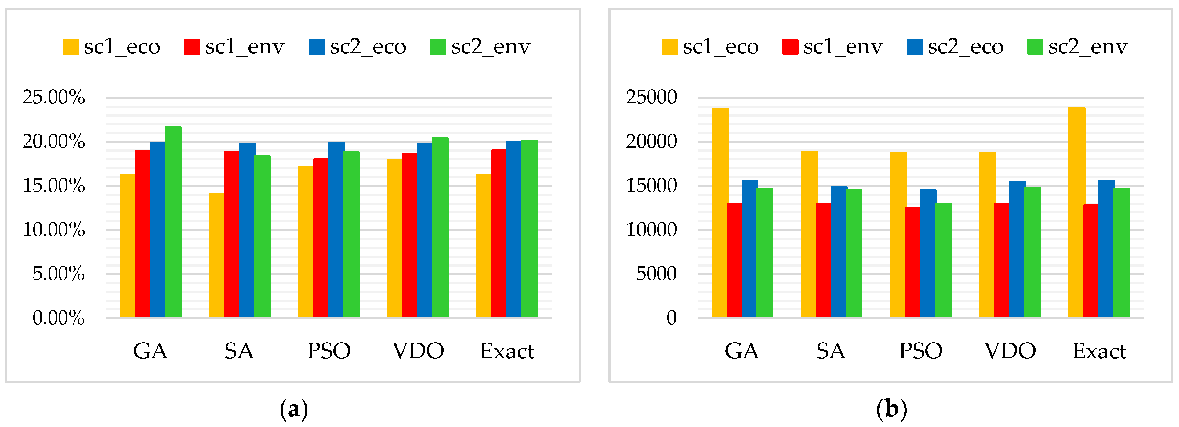
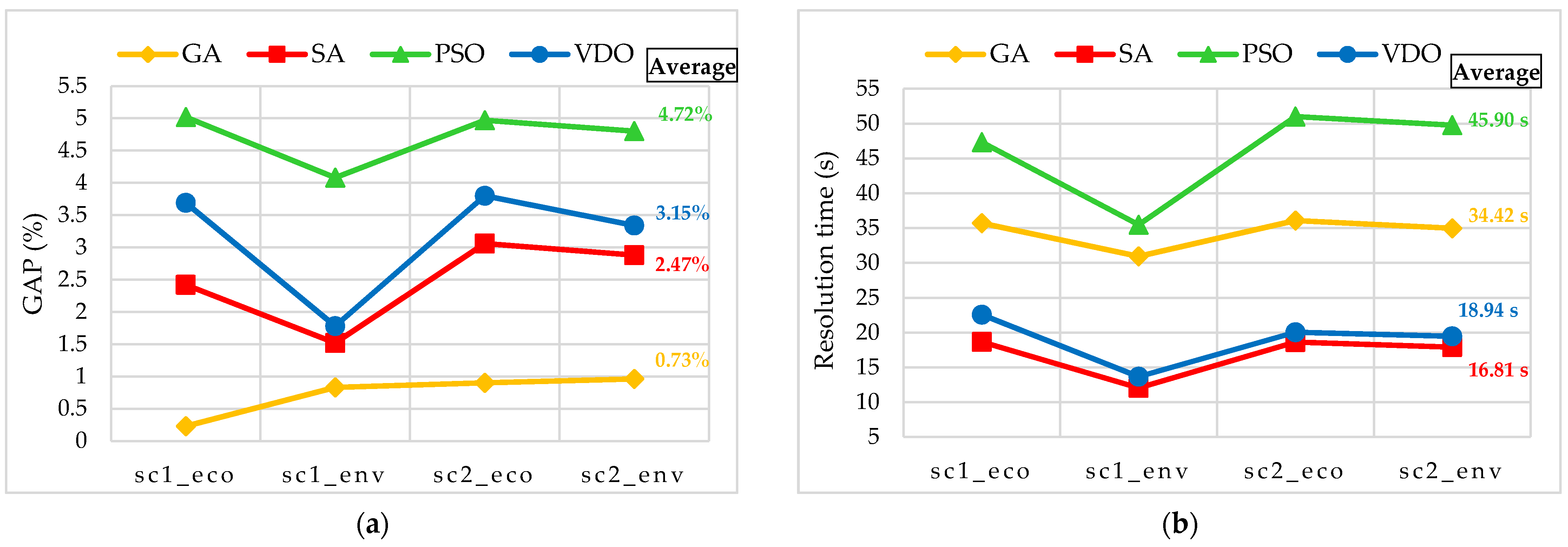
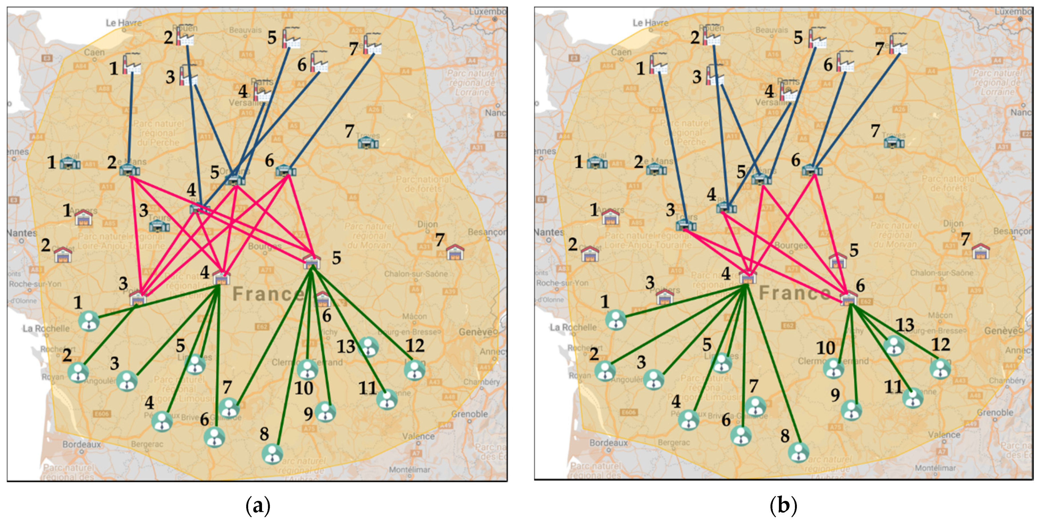
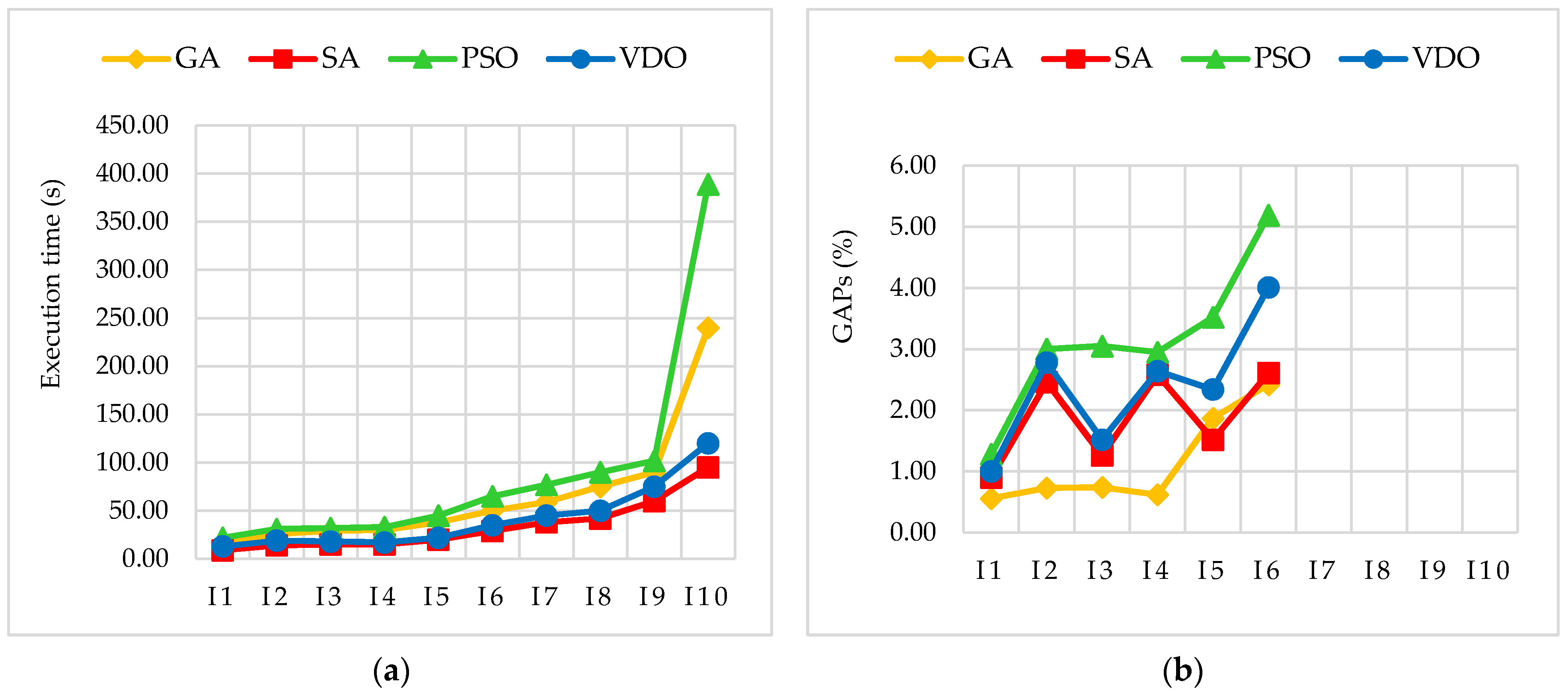
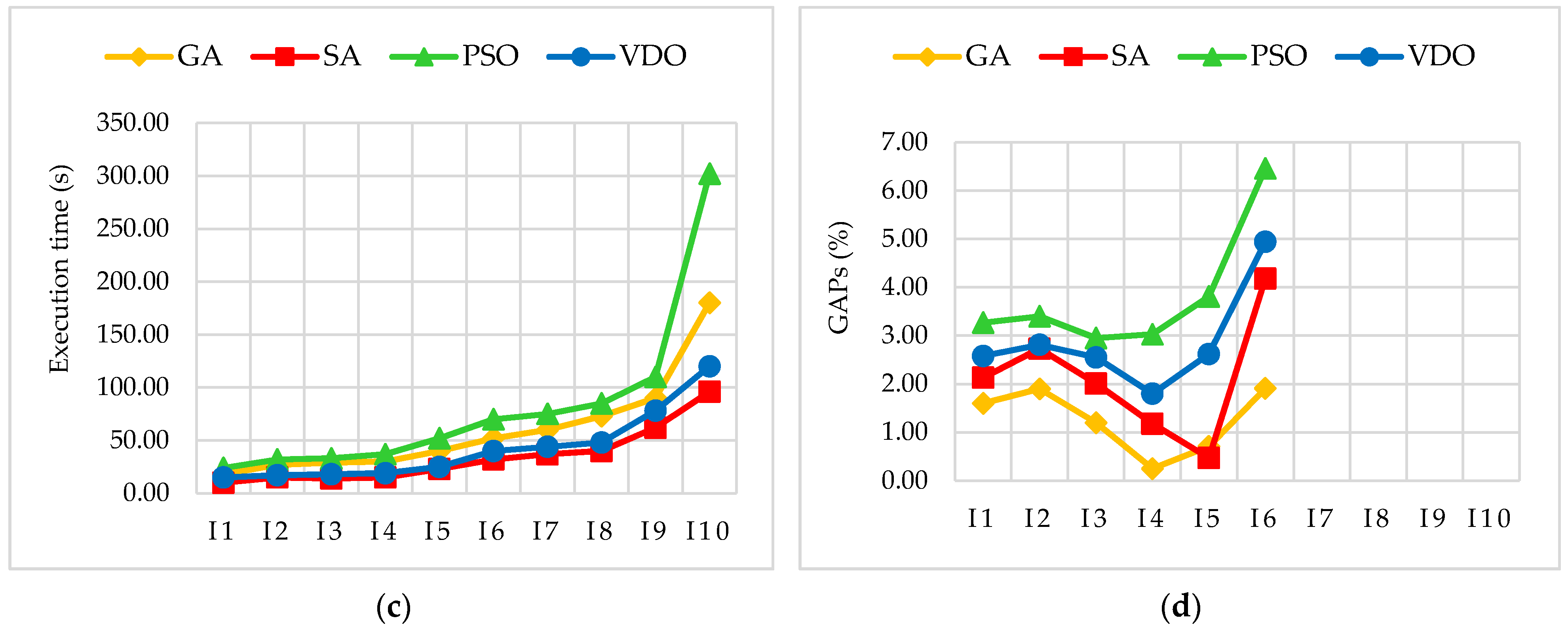
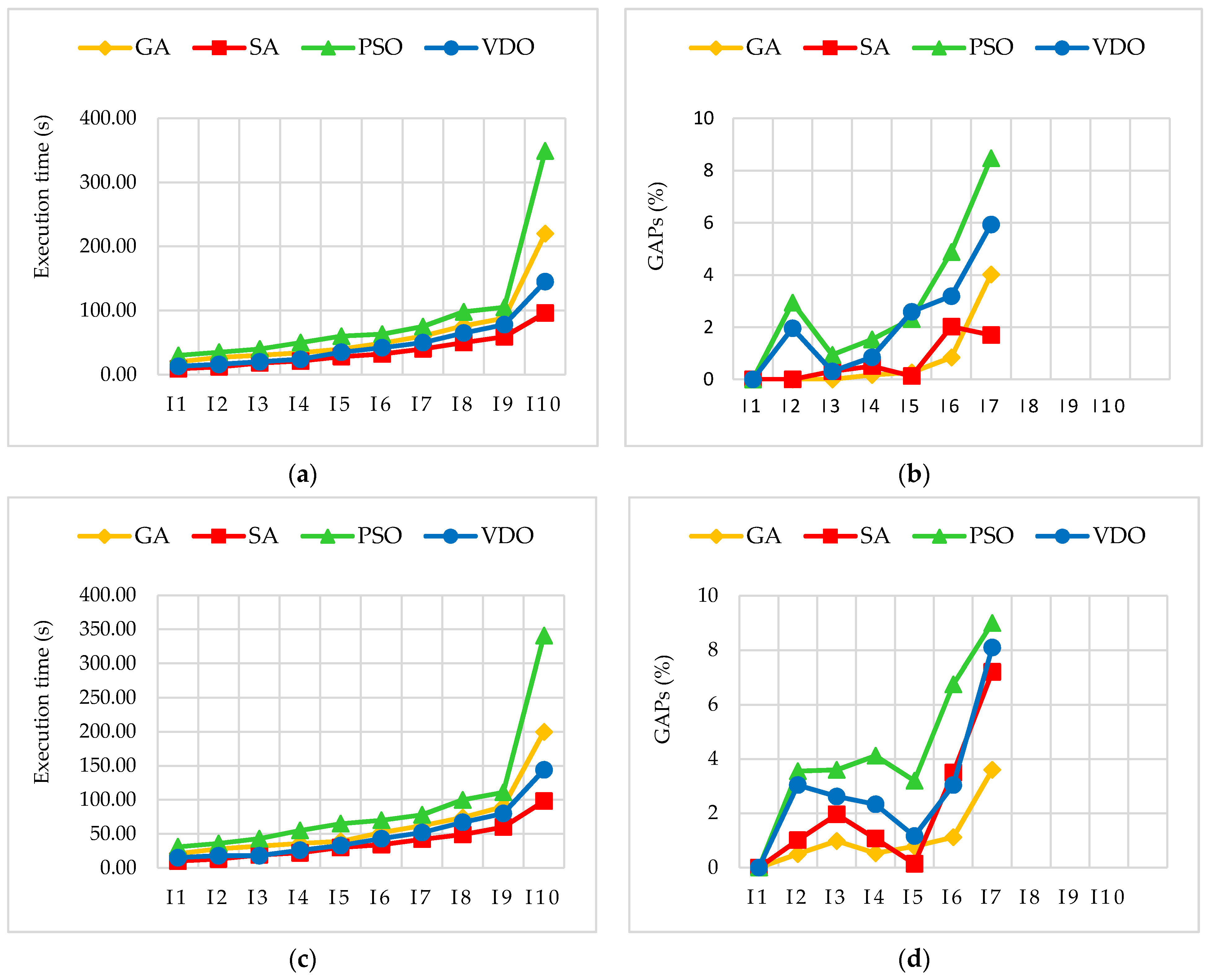
Publisher’s Note: MDPI stays neutral with regard to jurisdictional claims in published maps and institutional affiliations. |
© 2021 by the authors. Licensee MDPI, Basel, Switzerland. This article is an open access article distributed under the terms and conditions of the Creative Commons Attribution (CC BY) license (https://creativecommons.org/licenses/by/4.0/).