Article

Thermally and Dynamically Driven Atmospheric Circulations over Heterogeneous Atmospheric Boundary Layer: Support for Safety Protocols and Environment Management at Nuclear Central Areas

by
Larissa de Freitas Ramos Jacinto
1,
Luiz Claudio Gomes Pimentel
1,*,
José Francisco de Oliveira Júnior
2,
Ian Cunha D’Amato Viana Dragaud
3,
Corbiniano Silva
3,
William Cossich Marcial de Farias
4,
Edilson Marton
1,
Luiz Paulo de Freitas Assad
1,3,
Jesus Salvador Perez Guerrero
5,
Paulo Fernando Lavalle Heilbron Filho
5 and
Luiz Landau
3
1
Graduate Program in Meteorology, Federal University of Rio de Janeiro (UFRJ), Rua Athos da Silveira Ramos, 274, CCMN-Bloco G1, Cidade Universitária-Ilha do Fundão, Rio de Janeiro-RJ 21941-909, Brazil
2
Institute of Atmospheric Sciences (ICAT), Federal University of Alagoas (UFAL), Av. Paulo Holanda, 19-Cidade Universitária, Maceió, Alagoas 57072-260, Brazil
3
Civil Engineering Program, 149, Centro de Tecnologia-Bloco B, Federal University of Rio de Janeiro (UFRJ), Av. Athos da Silveira Ramos, Sala 101-Ilha do Fundão Caixa Postal 68506, Rio de Janeiro-RJ 21941-909, Brazil
4
Department of Physics and Astronomy, Alma Mater Studiorum-Università di Bologna, Via Irnerio 46, 40126 Bologna, Italy
5
Brazilian Nuclear Energy Commission (CNEN), Rua General Severiano, 84, Botafogo, Rio de Janeiro-RJ 22290-901, Brazil
*
Author to whom correspondence should be addressed.
Atmosphere 2021, 12(10), 1321; https://doi.org/10.3390/atmos12101321
Submission received: 30 July 2021 / Revised: 29 September 2021 / Accepted: 2 October 2021 / Published: 9 October 2021
(This article belongs to the Section Meteorology)

Abstract

:
Ilha Grande Bay is located in Angra dos Reis, Rio de Janeiro State, Brazil. The area is characterized by different land cover, complex topography and proximity to the Atlantic Ocean. These aspects make it susceptible to thermally and dynamically induced atmospheric circulations such as those associated with valley/mountain and land/sea breeze systems, among others. The Almirante Álvaro Alberto Nuclear Complex (CNAAA) is located in this region, with a total of two nuclear power plants (NPPs) in operation in the Brazilian territory, Angra I and Angra II. Therefore, knowledge of local atmospheric circulation has become a matter of national and international security. Considering the importance of the meteorological security tool as a support for licensing, installation, routine operation and nuclear accident mitigation, the main aim of this study is the development of combined strategies of environmental statistical modeling in the analysis of thermally and dynamically driven atmospheric circulations over mountainous and coastal environments. We identified and hierarchized the influence of the thermally and mechanically driven forcing on the wind regime and stability conditions in the coastal atmospheric boundary layer over the complex topography region. A meteorological network of ground-based instruments was used along with physiographic information for the observational characterization of the atmospheric patterns in the spatial and time–frequency domain. The predominant wind directions and intensity are attributed to the combined action of multiscale weather systems, notably, the valley/mountain and continent/ocean breeze circulations, the forced channeling due to valley axis orientation, the influence of the synoptic scale systems and atmospheric thermal tide. The observational investigation of the combined influence of terrain effects and meteorological systems aimed to understand the local atmospheric circulation serves as support for safety protocols of the NPPs, contemplating operation and environmental management. The importance of the study for the adequacy and skill evaluation of computational modeling systems for atmospheric dispersion of pollutants such as radionuclide and conventional contaminants can be also highlighted, in order that such systems are used as tools for environmental planning and managing nuclear operations, particularly those located in regions over mountainous and coastal environments with a heterogeneous atmospheric boundary layer.

1. Introduction

Nuclear fission began to be adopted for civil purposes in 1953, with the “Atoms for Peace” program, and was seen, at that time and during the 1970s Oil Crisis, as a possible, nearly unlimited energy source [1,2].
Currently, nuclear energy is used in 30 countries [3] and holds the potential to reduce not only dependence on fossil fuel-based energy sources but also undesirable emissions of greenhouse gases (GHGs) and precursor pollutants from photochemical oxidants and secondary aerosols, thereby contributing to climate change mitigation and reducing harmful effects on human health [4,5,6,7,8,9]. In comparison with other available low-carbon technologies, such as solar and wind, some advantages of nuclear energy are its high energy density through the occupation of smaller installed areas for the production of the same amount of energy [10,11,12] and its continued availability, providing energy security regardless of external factors such as environmental conditions and the amount of available reserves [13,14].
A potentially negative characteristic should be highlighted, that is, the severity of accidents in nuclear installations, which can occur during the operation of the reactors or in the transport of nuclear fuels [15]. Historic accidents, as observed on Three Mile Island, USA (1979), Chernobyl, Ukraine (1986), and Fukushima, Japan (2011), alerted the international community about the need to establish safety protocols with greater rigor for the operation of nuclear installations and new plant licensing [16,17].
The impact of the 2011 Fukushima accident led to a reduction in the construction of new nuclear units and the restriction of the use of nuclear energy in the global energy matrix [17,18]. The resumption of nuclear sector expansion is directly associated with the proposal of innovative strategies that contribute to increased safety in nuclear installations [18]. In Brazil, according to the National Energy Plan [19], an expansion had been planned that considered, in the most optimistic scenario, the construction of up to four new units in the country, in addition to the completion of Angra III at the Almirante Álvaro Alberto Nuclear Complex (CNAAA). However, after the Fukushima accident, the process was restricted to last only to the end of the construction of Angra III.
In 2011, the Specific Safety Guide for Meteorological and Hydrological Risk Assessment in Nuclear Installations [20] highlighted the main requirements and general recommendations on meteorological security tools as support for the nuclear area. According to these recommendations, in situ data should be collected following the standards of the World Meteorological Organization (WMO) [21]. The quality and homogeneity of this data should allow for the evaluation of extreme meteorological event occurrences and the detection of rarely occurring atmospheric phenomena that may pose risks to a nuclear facility; for example, if there is a long-time historical data series available, a climatological study including the analysis of extreme values should be carried out.
In environmental planning and management of nuclear operations, high resolution observational network, geotechnologies, numerical weather prediction and radionuclide dispersion modeling integrated systems are used (e.g., [22,23]). Measurements are the primary approach to better understand the atmosphere and they may also be used to investigate if model simulations properly describe the environment [24]. The numerical simulations are verified with observations through statistical metrics (e.g., [25,26]), frequency (e.g., [26]) and time–frequency (wavelet) analysis (e.g., [27]), wind roses (e.g., [28]), boxplots (e.g., [27]) and others.
It is worth noting that observational analysis can aid in determining the best configuration for numerical weather forecasting and pollution dispersion models, which should be implemented with enough spatial and temporal resolution to accurately represent the regional and local geophysical and meteorological characteristics of the area of interest, as well as the atmospheric multi-scale interactions. Careful consideration must be given to non-homogeneous locations and best modeling practices should be followed for the number of points in a horizontal direction, the number and distribution of vertical levels, the positioning of grid borders between themselves and, in relation to the complex terrain, the map projection, types of nesting (one-way or two-way), the use of high spatio-temporal resolution, parent grid ratio, time step, numerical stability considerations, adequate physical parameterizations, initial conditions and boundary conditions to non-homogeneous areas as time-varying sea surface temperature, land use and land cover, and topography high resolution databases [24,29,30,31].
Currently, 30 countries use nuclear energy and 28 are considering, planning, or working to include nuclear energy in their energy matrices. By 2019, there were 443 nuclear reactors in operation around the world: Europe, 182; Asia, 137; North America, 115; South America, 7; Africa, 2 [32]. A total of 89 nuclear reactors were placed in coastal areas without complex topography, 41 near complex topography but far from coastal areas and 58 nuclear reactors in coastal areas with complex topography (Figure 1), similar to CNAAA, indicating the study’s potential to support the development of meteorological hazards protocols in site selection evaluation and operation, according to [20]. Then, about 42% of the nuclear reactors in operation around the world are in regions with at least one of these complex physiographic characteristics.
In Brazil, the CNAAA, with the only two nuclear power plants (NPPs) in operation in the country, Angra I and Angra II, is also located in a coastal area at Ilha Grande Bay, Angra dos Reis in Rio de Janeiro State [33]. The area is characterized by different land covers, complex topography and proximity to the Atlantic Ocean, which make it susceptible to thermally and dynamically induced atmospheric circulations, such as those associated with valley/mountain and land/sea breeze systems, among others [34,35,36]. Moreover, interactions of the local atmosphere with the forced flow by synoptic scale systems can modulate the local flow and change the patterns of the wind regime in the region [37].
Therefore, observational scientific studies that are able to identify atmospheric patterns and generate supportive measured databases for assessing the ability of weather and climate forecast models to simulate complex terrain atmospheric flow are valuable. Such challenges motivated the realization of large-scale programs for the observational description and modeling of the flow in regions of complex terrain, among which are the following: VTMX (Vertical Transport and Mixing) campaign in Salt Lake Valley, Utah, United States of America (USA) [38,39]; MAP (Mesoscale Alpine Programme) in Riviera Valley, Switzerland [40,41]; the T-REX (Terrain-Induced Rotor Experiment) in Sierra Nevada, California, USA [42]; METCRAX (Meteor Crater Experiment) [43] and METCRAX II (Second Meteor Crater Experiment) [44] in Arizona, USA; the COPLEX (Cold-Air Pooling Experiment) in Shropshire, United Kingdom [45]; the MATERHORN (Mountain Terrain Atmospheric Modeling and Observations Program) in Utah, USA [46]. Additionally, multiple studies on radionuclide atmospheric dispersion from NPPs installed in coastal regions with complex topography have been performed in different localities: Cernavodă, Romania [47]; La Hague, France [48]; Hanbit, ex Yeonggwang, South Korea [49]; Diablo Canyon, USA [50]. The physiographic configuration of such regions is a great challenge to atmospheric modeling [51], which reinforces the importance of observational studies for a better understanding of mountain and coastal meteorology as applied to nuclear safety areas.
The diversity of NPPs installed in regions with physiographic characteristics similar to those of CNAAA is shown in Figure 1. In order to attend [20], it is indispensable to understand the growing trend for strict nuclear safety requirements for these areas, in addition to building a decision-making geographic information system platform by using a meteorological measurement network to simulate results in support of licensing, installation, routine operation and nuclear accident mitigation [33,52,53,54,55,56,57]. The analysis of meteorological conditions in these areas is very important to evaluate and mitigate the risks associated with natural hazards. The regions should be well characterized to mitigate the impact of extreme environmental events [20,58] and the winds are considered as one of the main meteorological variables for this evaluation. While high wind intensity impacts the operation of NPPs [59], lower wind speeds have strong effects on the dispersion of radioactive materials [60]. According to [61], local winds also influence the dispersion of this material. Regarding the dispersion, there are also a lot of studies evaluating its relationship with the stability in complex mountain and coastal areas (e.g., [62]).
The WMO [63] examines the problems that emerge at various types of NPP sites and discusses issues related to atmospheric diffusion. The analysis of sites with special effects on atmospheric diffusion is extremely challenging. Examples of sites with special atmospheric diffusion effects are as follows: sites with complex terrains, such as narrow hills and valleys; coastal sites in general and particularly those with complex topography (e.g., a ridge inland or mountain), an island beyond and another coast beyond the water; sites near built-up areas.
Land-surface heterogeneity continues to be an open challenge for understanding and predicting from microscale to synoptic scale atmospheric dynamics and hilly terrain add complexity to this issue [30], since a generalized treatment is not viable due to the flows being highly site-dependent.
Therefore, the main goal of this study is to combine statistical modeling strategies for the analysis of thermally and dynamically driven atmospheric circulations over mountainous and coastal environments, to serve as support for safety protocols for the NPPs. To better understand these processes and meteorological systems over non-homogeneous area is important, because similar conditions are observed around worldwide regions where NPPs are installed.
The remainder of this paper is organized as follows: In Section 2, the materials and methods are outlined, describing the study area, data analyzed and techniques applied to compose the combined statistical modeling strategies. In Section 3, the main results are presented and discussed. Finally, conclusions are summarized in Section 4.

2. Material and Methods
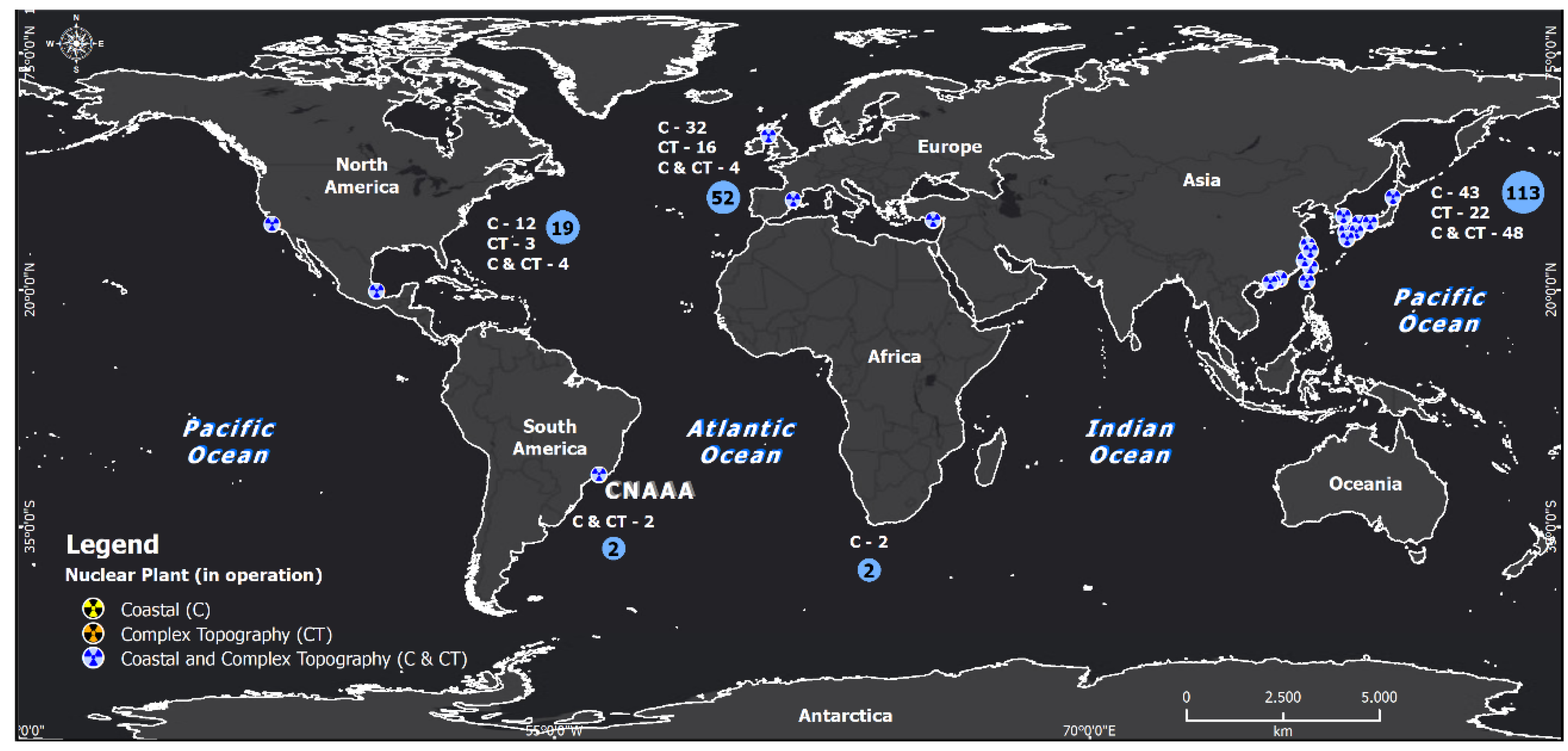
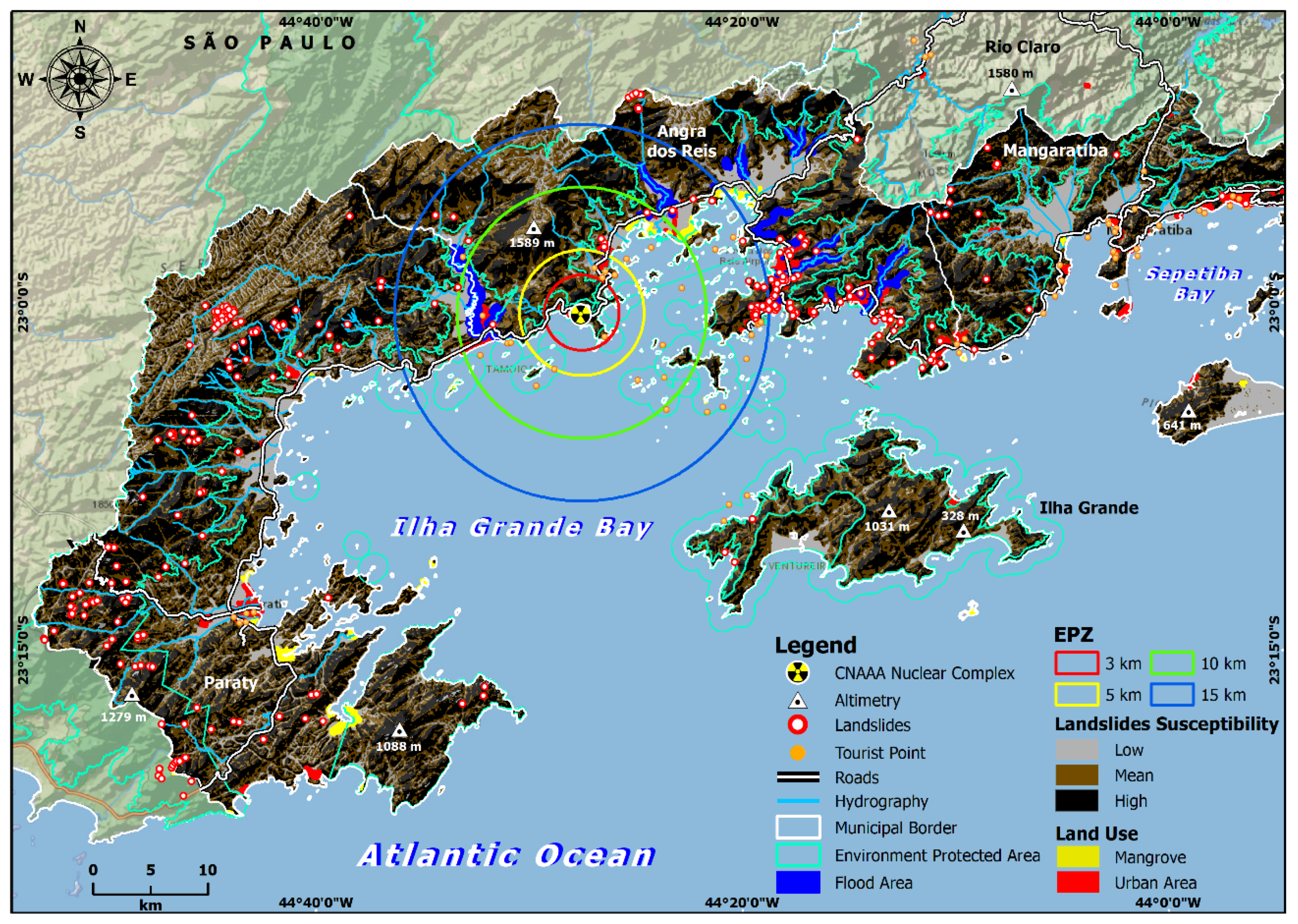
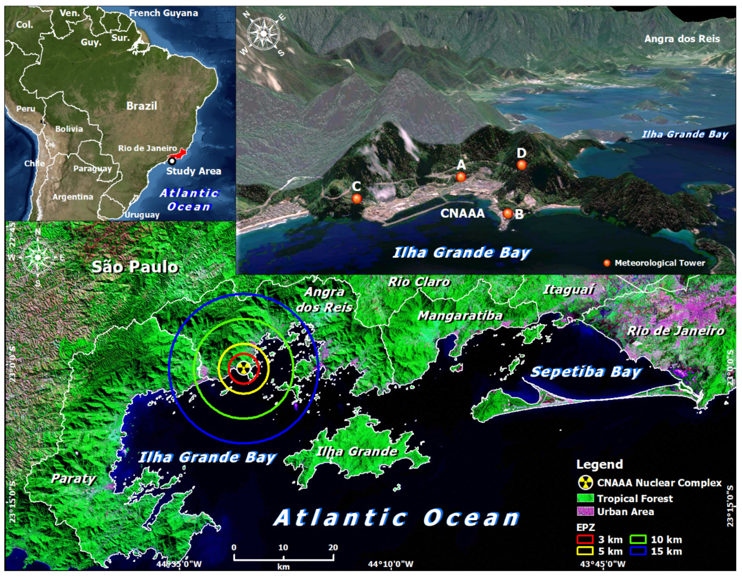
This scientific study’s methodological approach, besides supporting NPPs’ safety protocols by observational investigation, presents a universalist character and can be extended to other regions of the world with potential capacity for installing NPPs, contemplating safety protocols of the units already in operation and environmental management. The importance of this study for the adequacy and skill evaluation of computational modeling systems for atmospheric dispersion of pollutants as radionuclide and conventional contaminants are also highlighted, as such systems are used as tools for environmental planning and managing nuclear operations, particularly those located in regions over mountainous and coastal environments with a heterogeneous atmospheric boundary layer. The CNAAA area is characterized by different land covers, complex topography and proximity to the Atlantic Ocean, which make it susceptible to thermally and dynamically induced atmospheric circulations, such as those associated with valley/mountain and land/sea breeze systems, among others [48,49,50]. Moreover, interactions of the local atmosphere with the forced flow by synoptic scale systems can modulate the local flow and change the patterns of the wind regime in the region [51].

2.1. Study Area

The city of Angra dos Reis, located on the south coast of Rio de Janeiro State in the southeastern region of Brazil, has an area of 813.210 km2 and a population of 207.044, with a demographic density of 254.6 inhabitants/km2 [64]. Currently, because the city houses the CNAAA, with Angra I and Angra II being the only operating nuclear plants and Angra III being under construction, nuclear power serves as one of the most important economic sectors, together with the naval and oil industries.
The CNAAA is installed at Itaorna Beach, a coastal region with a narrow continental strip at the bottom of Ilha Grande Bay (Figure 2). In addition, the plant is surrounded by the Serra do Mar mountain range, formed by high mountains and hills with high declivity [23], as shown in Figure 2. The physiographic characteristics of the region provide the formation of local circulations of sea/land and valley/mountain breezes, in addition to orographic gravity waves [65]. Moreover, the local atmosphere may also be influenced by the synoptic scale systems that modify the circulation patterns in the region. According to [66], the typical meteorological systems that influence the Rio de Janeiro State are the South Atlantic Subtropical Anticyclone (SASA), the South Atlantic Convergence Zone (SACZ), frontal systems, instability lines, atmospheric blocking and mesoscale convective systems.
Among the nuclear safety protocols aimed at the protection and public safety, the projected emergency planning zones—EPZ (3, 5, 10 and 15 km)—in the region surrounding the CNAAA are part of the local management structure, aiming at the preparation and prevention of actions in case of accidents and emergency procedures. Different features of the region demonstrate its spatial and socio-environmental complexity, which impact not just the surrounding residents, but the entire local dynamics, and must be analyzed holistically [33,37,52,53,54,55,65,67,68]: meteorological and climatological factors, such as wind and rain, have a direct impact on radionuclide dispersion and fog incidence; geological-geomorphological factors, such as relief slopes and susceptibility to constant mass movements and floods; urban mobility factors, such as precarious road structures, sloping areas, and narrowing roads, make it difficult for the population to move around; environmental, with numerous protected areas, tropical forest vegetation, and several water bodies.
The methodological procedures and structure of the analyses are summarized in the flowchart presented in Figure 3.

2.2. Data and Study Period

The combined statistical modeling strategies are based on an analysis of the time series data recorded in the CNAAA meteorological monitoring network, composed of four meteorological towers (A, B, C and D) installed at strategic points in the nuclear complex (Figure 2). The towers were positioned at different altitudes with regard to the mean sea level. The positioning of each tower with respect to topography is shown in Figure 2. The measurements for tower A were recorded at three different heights in relation to its base, 10, 60 and 100 m, hereafter denoted as levels A-10 m, A-60 m and A-100 m, while, for the other towers, the measurements were taken at a height of 15 m in relation to the base of each tower (Table 1), hereafter denoted as levels B-15 m, C-15 m and D-15 m.
The data comprise two distinct periods. The first period corresponds to the years between 01/05/1982 and 01/01/2002, with hourly wind data measured at all towers (A, B, C and D). The second period covers 2016 and includes meteorological data (temperature and wind) recorded at the three heights of tower A, with a 15 min temporal resolution. Data from 2002 to 2016 is missing, resulting in a gap in the data analysis period. It is related to a policy of public access to these data by agencies of the Brazilian nuclear sector. However, as the CNAAA region is inserted in an environmental protection area, few changes in the land surface have been observed in the gap period. Then, the analysis of past years can be considered for the climatological characterization and used for safety protocols anyway.

2.3. Quality Control of Wind and Temperature Meteorological Data

It should be noted that the recorded meteorological data can present some unrealistic values owing to occasional sensor failures. To address this, the data were evaluated by applying filters, using the techniques proposed by [69] and the potentially unrealistic values were removed, as follows. The air temperature data were filtered by removing data that were incompatible with the sensor threshold. To do this, a threshold between −10 °C and 50 °C was established for the temperature data, as recommended by the Brazilian Nuclear Energy Commission (CNEN) [70]. A filter to detect the absence of variability in consecutive data was then applied to the wind and temperature data. From this, we removed records in which the wind intensity and direction remained unchanged for more than 2 h. Temperature data that presented a persistent lack of variability for more than two days were also removed. The final percentage of valid data was higher than 61% in the period from 1982 to 2002 and higher than 96% in 2016.

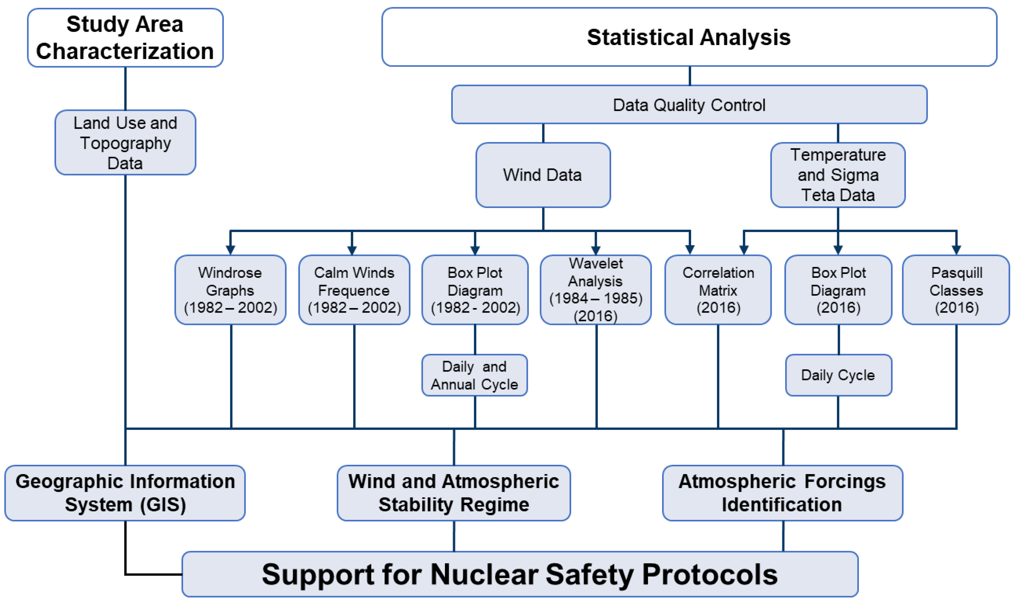
2.4. Techniques Composing the Combined Statistical Modeling Strategies

The statistical techniques used in the modeling system to evaluate the wind regime and stability class of the local atmosphere are described in this section.
Based on wind roses and box plot diagrams, a climatological characterization of the wind regime was made for the period 1982–2002. The wind rose analysis allowed for the identification of the predominant wind directions and intensities, in addition to the calm regime, considering a daily cycle as follows: early morning (from 12 a.m. to 5 a.m.), morning (from 6 a.m. to 11 a.m.), afternoon (from 11 a.m. to 5 p.m.) and evening (from 6 p.m. to 11 p.m.). The calm regime was considered for winds with an intensity lower than 1 knot or 0.515 m·s−1 [71]. Exploratory statistics were applied based on the boxplot graph, composed of the mean, median, 1st quartile, 3rd quartile, interquartile range and extreme values (outliers) [72], to assess the hourly and seasonal variation in wind intensity.
The identification and hierarchization of the main drivers of the wind were performed via wavelet analysis, as described by [73]. This technique allows for the decomposition of a time series into a time–frequency domain, thereby determining the dominant frequencies and how the associated modes of variability vary over time [74]. It can be applied to a wide range of atmospheric science phenomena. According to [75], the wavelet transform has been basically used in two ways, namely, as an integration nucleus of the analysis to obtain information about the processes and/or as a characterization basis of the processes. In this way, the wavelet transform is used in this study to evaluate the frequency in which the greater powers of the wind components are observed, which allows to specify the contribution of local and synoptic meteorological systems as wind forcing. The wavelet analysis, based on observed wind data, can also be used as support to properly configure an atmospheric modelling system, since the temporal scales are previously determined.
Wavelet analysis used in this work is based on the methods given by [74], with wavelet bias rectification from [76]. Because this technique is often used to analyze geophysical data [76], the Morlet wavelet was chosen as the wavelet base function. The averaging over time was calculated over all local wavelet spectra, producing the global wavelet spectrum [74]. A wavelet analysis was then be applied to the zonal (u, m·s−1) and meridional (v, m·s−1) wind components measured at the CNAAA towers from 1 February 1984, to 1 September 1985 and for the full year of 2016. The first period corresponds to the portion with the highest availability of data in the full set (1982–2002) for climatological characterization. The second one was considered because it is the latest period of data available.
The analysis of the atmospheric stability indexes was based on the vertical temperature gradient and standard deviation of the wind direction fluctuations using the dataset for the year 2016. Correspondence between the ranges of values in the stability indexes and the Pasquill stability classes was applied according to the CNEN Standard for the Meteorology Program [70]. The thresholds are listed in Table 2.
The distribution of the atmospheric stability parameters was performed via boxplot graphics, which provided information on the mean and data distribution variability. The use of wind roses and a boxplot allowed us to perform a daytime assessment of the pattern of meteorological variables. In addition, a description of the local pattern of the wind and stability regime was produced, providing subsidies for the identification of mechanical and thermal flow forces.
A statistical analysis via the correlation matrix was applied to the wind (direction and speed) and stability dataset for 2016. Because the dataset had linear and circular variables, several correlation coefficients were applied depending on the type of variables related. The Pearson correlation coefficient was used to assess the similarity between linear variables. This coefficient corresponds to the ratio between the covariance of two variables (Cov [x, y]) and the product of the standard deviation between both variables [72], as shown in Equation (1):
ρ = C o v ( x , y ) σ x σ y
The linear–circular correlation coefficient was used to assess the relationship between a circular variable and linear variable [77,78]. This formula is given by a combination of the correlations between the linear variable and the sine and cosine values of the circular variable in Equation (2):
r x θ = r x c 2 + r x s 2 2 r x c r x s r c s 1 r c s 2
where rxc, rxs and rcs are computed using Pearson correlations, given by
r x c = c o r r ( x , cos ( α ) )     r x s = c o r r ( x , s i n ( α ) ) ,       r c s = c o r r ( c o s ( α ) ,   s i n ( α ) )
Finally, the circular–circular coefficient indicates the degree of similarity between two circular variables and β [78,79,80], as shown in Equation (3):
r c , n = i = 1 n s i n sin ( α i α _ ) s i n sin ( β i β _ )   [ i = 1 n sin 2 ( α i α _ )   ]   [ i = 1 n sin 2 ( β i β _ ) ]  
where the mean angles ( α _   and β _ ) are computed as follows:
S = i = 1 n s i n ( α i )   ,         C = i = 1 n c o s ( α i )   ,   R = C 2 + S 2
α _ = { ( S / C ) ,     i f   C 0   ;   ( S / C ) + π ,   i f   C < 0   ;   U n d e f i n e d ,     i f   R = 0        

3. Results and Discussion

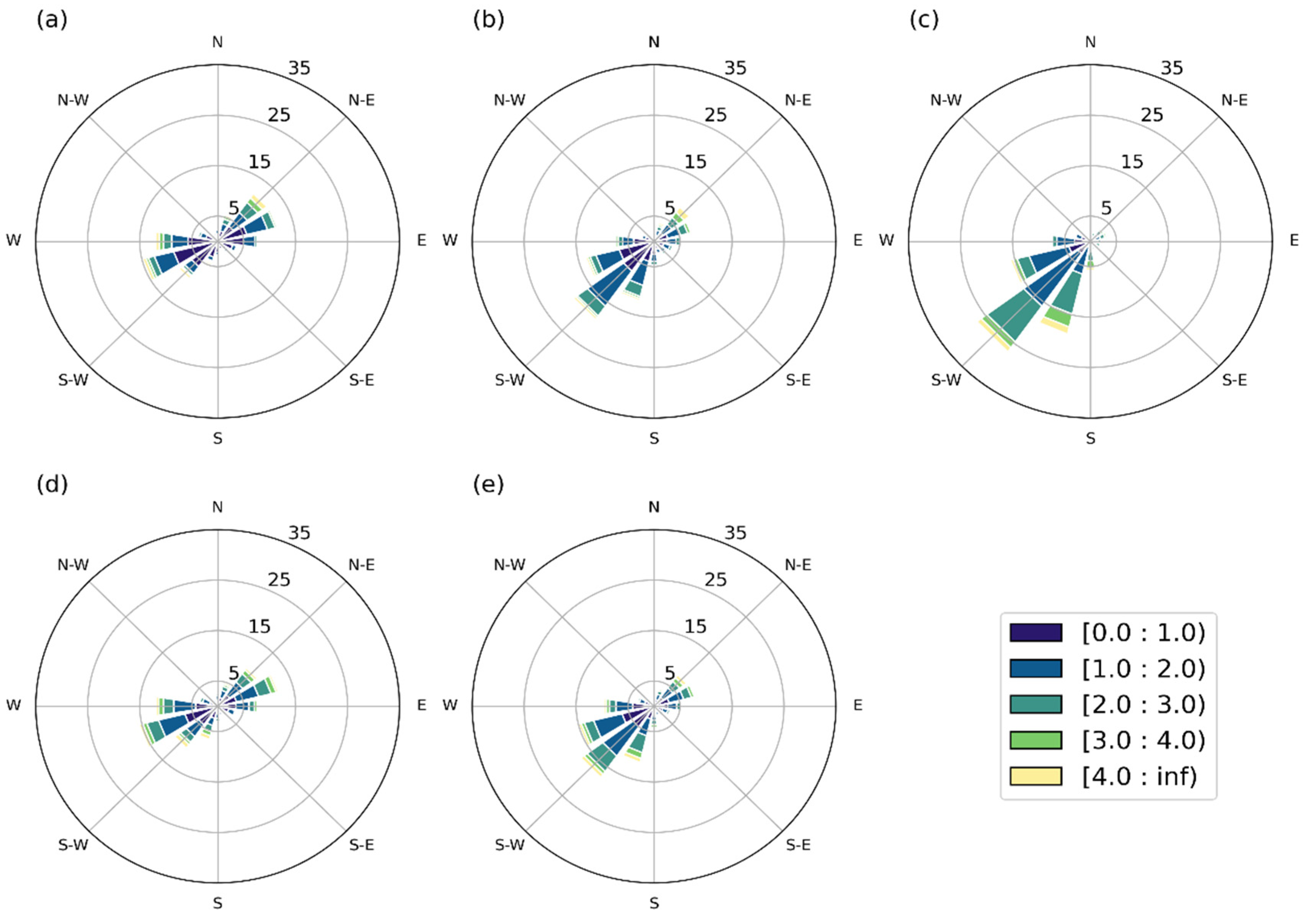
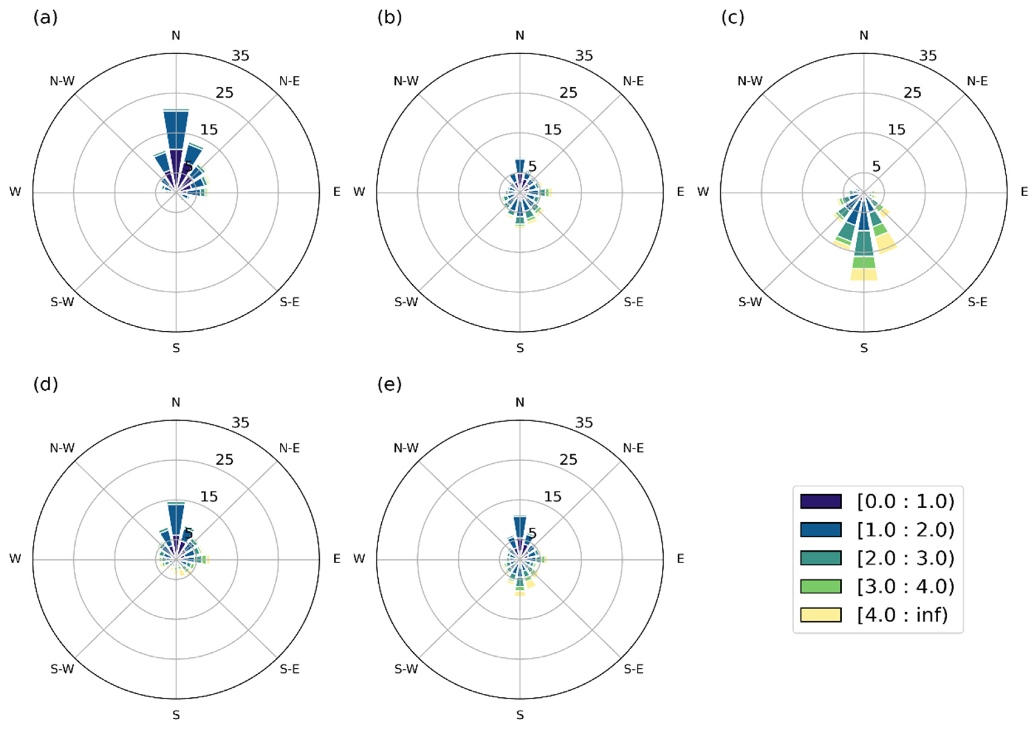
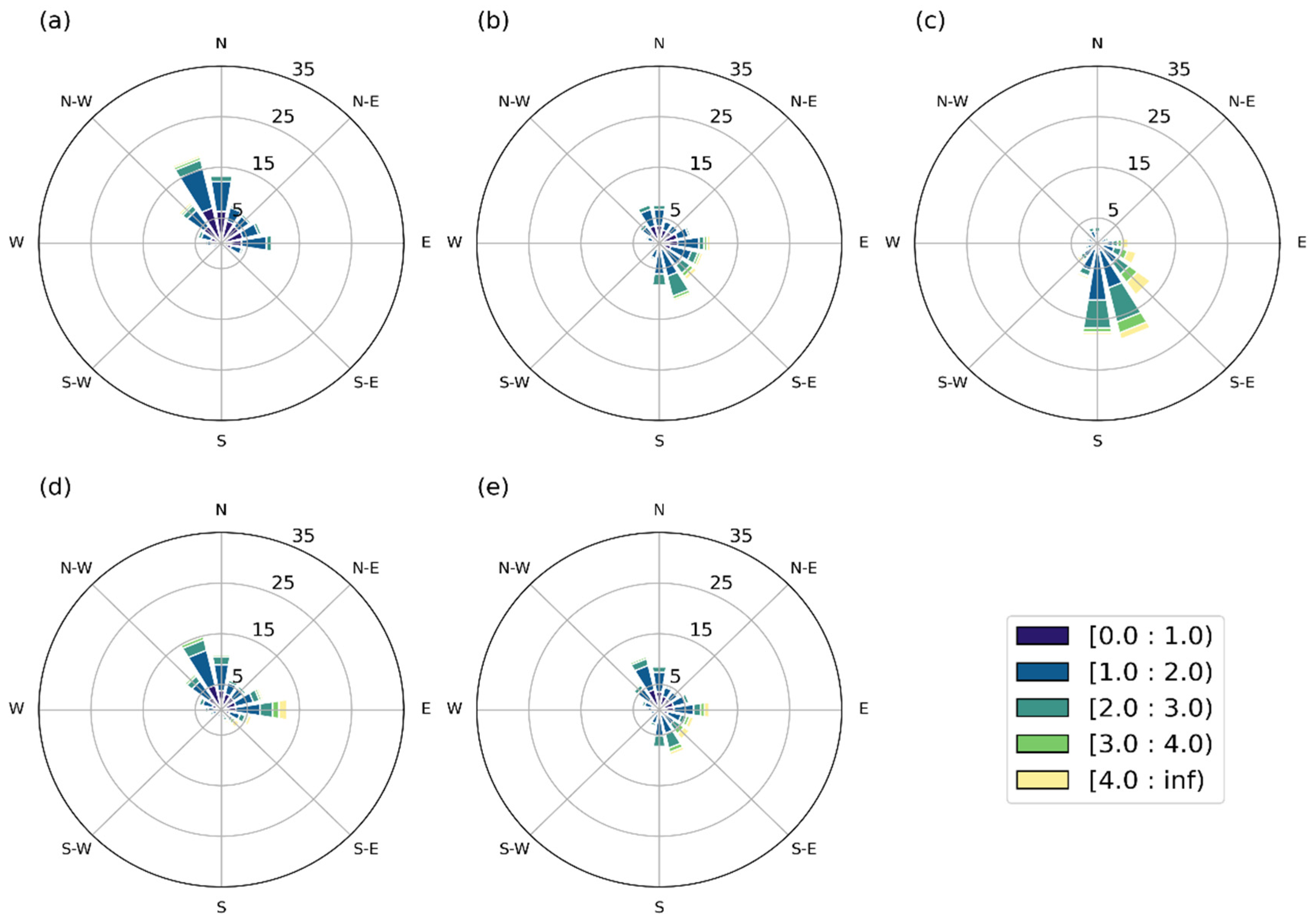
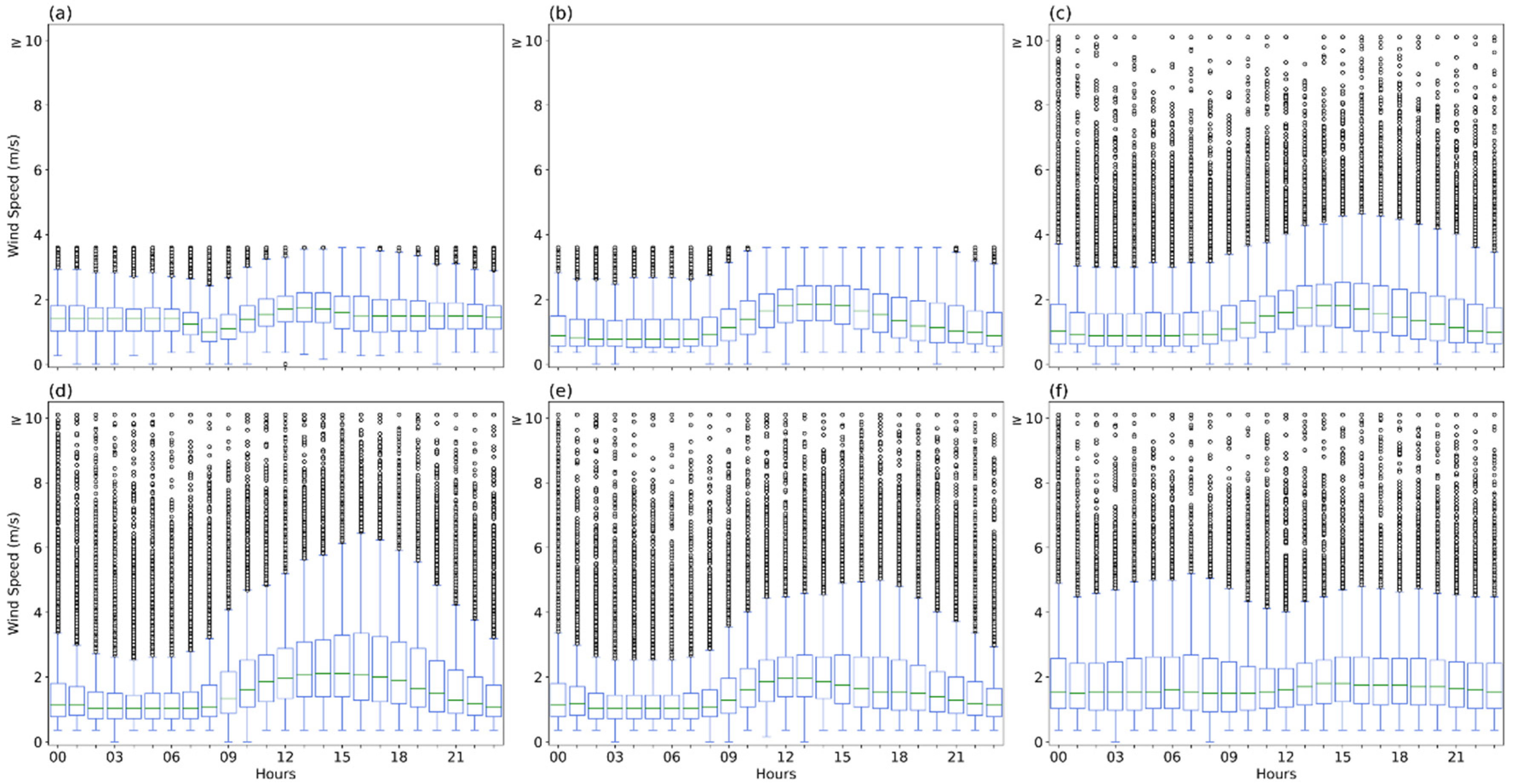
3.1. Analysis of Local Circulation: Temporal Domain Analysis

Figure 4, Figure 5, Figure 6, Figure 7, Figure 8 and Figure 9 present the wind roses for all towers and measurement levels. The indices from (a) to (d) of all figures correspond to the daily periods, that is, early morning, morning, afternoon and evening, respectively. The wind roses represented by index (e) show the all-day composition of each anemometer.
The analysis of the total wind composition for A-10 m indicates a predominance of the north (N) direction (Figure 4e), with considerable contributions from the north–northeast (NNE), southwest (SW) and south–southwest (SSW). In the early hours of the morning, the N sector was predominant (54%), followed by the NNE direction (18%), with winds varying between 1 and 3 m·s−1 (Figure 4a). The first predominant direction is related to the thermal forcing associated with the cooling process of the mountain range covered by vegetation, compared to the surroundings (mountain breeze). The second predominance, in addition to the influence of local thermal forcing, is associated with the SASA, which induces northeast (NE) winds in the Brazilian Southeast region [81,82].
In the morning, the N (20%) and NNE (12%) directions were maintained, in combination with the SSW (18%) and SW (12%) directions, again with winds between 1 and 3 m·s−1 (Figure 4b). This pattern recorded in the morning showed that there was a transition period, with the coupling of the winds in the NNE from mountain breeze circulation and SASA, with SW winds caused by the sea and bay breeze formation. In the afternoon, there was a predominance of the SSW (30%) and SW directions (25%) (sea and bay breezes), with an increase in wind intensity that reached maximum values of approximately 4 m·s−1 (Figure 4c). In the evening, the frequency of the N sector increased again, with N (about 40%) and NNE (20%) directions and intensity below 3 m·s−1 (Figure 4d).
The wind regime at A-60 m and A-100 m were similar to each other. There was a predominance of winds in the NE–SW axis due to the daily cycle (Figure 5 and Figure 6). In the evening and early morning, the prevailing directions were NE and east–northeast (ENE) (between 12% and 15% in each direction), followed by west (W) and west–southwest (WSW) (approximately 12%), with an intensity between 1 and 3 m·s−1 (Figure 5a,d and Figure 6a,d). In the morning and afternoon, there was a higher frequency of SW winds (approximately 25%), followed by SSW (between 15% and 25%) and WSW (12%) directions, with wind speeds greater than those in the evening and early morning, mainly in the afternoon, when the A-100 m winds were greater than 4 m·s−1 (Figure 5b,c and Figure 6b,c). The analysis of the tower wind roses indicates a trend of wind rotation in the clockwise direction of approximately 45º, from the lowest level (A-10 m, Figure 4) to higher levels (A-60 m and A-100 m, Figure 5 and Figure 6). The occurrence of winds from W/WSW observed at A-60 m and A-100 m in the early morning, morning and evening (Figure 5 and Figure 6) was not registered close to the surface, at A-10 m (Figure 4). Moreover, during the early morning and evening, the winds from NNE were predominant at A-10 m (Figure 4), while, for the same period, there was a predominance of NE–ENE winds at A-60 m and A-100 m (Figure 5 and Figure 6). The higher contribution of the zonal components at A-60 m and A-100 m may be related to the contribution of the flow channeling between the slopes surrounding the region. This mechanism was described by [35,36] for other areas influenced by topographic configuration, in addition to the interaction of thermally induced flow with topographic barriers.
The analysis of the total composition of B-15 m winds indicates a flow with a directional pattern distributed in all sectors and winds notably less than 3 m·s−1, mainly in the N sector (Figure 7e). The greatest wind speeds occurred in the afternoon, in the order of 4 m·s−1 when the directions were mostly between the SW and SE sectors (Figure 7c). The early morning period was characterized by less intense winds (<2 m·s−1), with a predominance between the NW and NE sectors (Figure 7a). In the morning, there was a uniform pattern of wind direction distribution, that is, the direction distribution occurred in practically all sectors, with a slight predominance for sectors N, E, S and SSE, with a frequency of 6–10% (Figure 7b).
At C-15 m, the NNW, E and SSE directions stood out, with a frequency between 6% and 10% (Figure 8e). In the evening and early morning, the wind regime was similar, with an intensity range of 0–4 m·s−1 (Figure 8a,d). In the morning, winds were predominant in the NNW, E and SSE sectors (Figure 8b). Overall, at B-15 m and C-15 m, the winds presented a pattern similar to that observed at A-10 m, with a predominance of weak N winds in the early morning, associated with the katabatic wind. Then, in the morning and afternoon, there was a decrease in the frequency of occurrence of sector N and a progressive increase in the SSW, S, SSE and SE directions at B-15 m and C-15 m, indicating the wind rotation and the beginning of the sea breeze and bay forcing (Figure 7b,c and Figure 8b,c). The hypothesis about the contribution of thermal forcing to the flow at A-10 m, B-15 m and C-15 m can be evidenced by the flow analysis, combined with the terrain elevation analysis (Figure 2). Moreover, this hypothesis is reinforced by the wavelets analysis of the southern components of these three sites (A-10 m, B-15 m and C-15 m), as will be discussed in Section 3.2.
It is also worth mentioning the importance of the cooling/heating mechanism in the configuration of the daily wind cycle at A-10 m, B-15 m and C-15 m, followed by other mechanisms that may occur simultaneously with the thermal forcing, mainly induced by the interaction of the wind with the relief of the region, which justifies, for example, the contribution of the E direction in the flow observed at B-15 m and C-15 m.
Tower level D-15 m had a total wind pattern characterized by the directions W and NE, with speeds exceeding 4 m·s-1 (Figure 9e). In the early morning and morning, the predominance of the direction was W and NNE (Figure 9a,b). With the diurnal evolution, there was a gradual increase in the occurrence frequency of the wind from the W in the afternoon (Figure 9c). In the evening (Figure 9d), the distribution pattern was similar to that recorded during the early morning and morning. At that point, the flow of the mountain could be attributed to the predominance of the wind in the NE direction during the periods of early morning, morning and evening, while, for the predominant direction of W and SSW during the afternoon, there was a contribution of the flow of the sea breeze and bay. The W direction appeared in all periods (Figure 9); however, the occurrence of this component experienced an increase in the period of greatest heating (afternoon) (Figure 9c).
This observation indicates the possibility of several forcing mechanisms inducing flow in this direction at that point. As pointed out in the case of A-60 m and A-100 m, the flow from W at D-15 m may be associated with the contribution of the flow between the slopes and the interaction of the flow with the topographic barriers, such as the possibility of forced channeling through the terrain [34]. In addition, due to the positioning of this point at a 305 m altitude, a possible turn with the height of the predominant direction generated by the thermally induced circulation cells should be considered. This could explain a possible contribution to the predominance of W–WSW in the afternoon (sea breeze) at D-15 m, while, at the other tower site, the sea breeze could be attributed, in general, to the directions of SW, SSW and S. Thus, it can be said that the bimodal behavior of the wind direction at D-15 m, which had little influence on the NE–W pattern throughout the daily cycle, was influenced by the combination of thermal and dynamic mechanisms that affected the wind regime at that point.
It is worth mentioning that the wind roses from all tower sites (Figure 4, Figure 5, Figure 6, Figure 7, Figure 8 and Figure 9) show records of wind directions between NNE and E. In addition to the contribution of the local factors mentioned above (i.e., channeling processes and breeze circulations), such registers can also be associated with an eventual influence from the SASA, which typically induces first quadrant winds in the state of Rio de Janeiro [82,83].
The contribution of local factors inducing different wind directions at the CNAAA and the heterogeneity of circulation patterns observed between the tower sites have been identified from previous studies of the region [65,84,85]. It is worth mentioning that the local daytime cycle patterns analyzed through the 1982–2002 database period were also observed in the 2016 database period (figures not shown).
Table 3 shows the percentages of calm wind conditions at the six measurement tower sites. Considering the all-day period, A-60 m had the highest percentage of calm winds, with a total of 12.58%, followed by A-100 m (11.86%). On the other hand, the lowest level of tower A (A-10 m) had the lowest percentage of calm (4.07%). These percentages indicate that the persistent katabatic wind is of considerable importance to the minor records of calm winds close to the surface.
In relation to the day cycle, the highest percentages of calm winds occurred during the early morning, except for those recorded at A-10 m and D-15 m, where the highest percentage of calm winds occurred in the morning. In the early morning, A-60 m and A-100 m again had the highest calm percentages, with 24.24% and 20.26%, respectively. It is also noteworthy that A-10 m had the lowest percentage at all times, when compared with the other measurement tower sites in the same period. In general, the percentage of calm winds had the highest values during the early morning, then the values decreased sharply with the lowest values in the afternoon and gradually increased again in the evening.
Figure 10 presents the wind roses for the registers of winds above 17 m/s at A-100 m, B-15 m, C15 m and D-15 m, which corresponds to 0.01, 0.05, 0.04 and 0.03% of the data recorded between 1982 and 2002. According to [21], winds between 17 and 20.7 m/s are responsible for damage such as breaks twigs off trees. This document also mentions that, with higher wind speeds, the impacts can be occurrences such as trees uprooted and even structural damage in buildings.
It is noteworthy that the most intense wind records occur in all directions (Figure 10), reinforcing that these wind gusts are not related to only a single meteorological phenomenon. These values of more intense winds can be associated with the influence of meteorological systems, such as the frontal system, local convection, SACZ, SASA, or local storms, which are known to intensify the winds in the study region [66,86].
In addition, the possible relationship between wind gusts episodes and storm events highlights the demand to use tools targeting the nowcasting. The IAEA [20] recommends that weather radar and satellite images may be advantageous for monitoring storms potentially dangerous, supporting the EPZ in case of accidents and emergency procedures.
Figure 11 illustrates the hourly distribution of wind intensities for each of the existing weather towers at CNAAA via a boxplot. In general, all tower sites and times had a median distribution below 2 m·s−1 throughout the day and in at least 75% of records (3rd quartile), the intensity values were less than 3 m·s−1. In addition, the difference in the average speed recorded throughout the day is highlighted. In the early morning and morning periods, the lowest speed values were recorded in the A tower site (10 m, 60 m and 100 m), B-15 m and C-15 m, but not at D-15 m. At A-60 m, A-100 m, B-15 m and C-15 m, based on the data median, it was found that there was an asymmetric distribution of the records, indicating that, although there were records above 3 m·s−1 at these points, half of the data distribution was made up of records smaller than 1 m·s−1. There was still less variability in the A-100 m, B-15 m and C-15 m values found between the 25th and 75th percentiles.
At 7 a.m., the wind speeds began to intensify and this would occur until mid-afternoon, owing to the circulation of sea and bay breezes, as well as to the position of the intersection between the continental surface and the sea surface, at B-15 m (2.4 m·s−1) and C-15 m (2 m·s−1), with the highest average speed in the afternoon. After this period, speeds decreased in the evening and early morning, when the flow at these tower sites had a greater contribution from the katabatic winds.
For A-10 m, the distribution of data at 8 a.m. indicated a slowing down of winds at this time, compared to the other times of the day. This result corroborates that presented in Table 3, which indicates a higher record of calm at A-10 m in the morning. This higher frequency of less intense winds from the early morning, followed by a gradual increase in the wind intensity from 9 a.m., could be related to the process of de-intensifying the katabatic breeze at the beginning of the morning and the process of formation and intensification of circulation sea and bay breezes throughout the morning.
At D-15 m, there was no evident daily cycle in wind speed (Figure 10f). The difference between the variability identified at D-15 m and the other tower site is due to the positioning of the sensor at 305 m in altitude [37], which contributed to the occurrence of even more intense winds in the evening and early morning. The results obtained from the calm and average speed at D-15 m corroborate those described by [65,84].
As previously highlighted, the records of all tower sites indicated the predominance of low-intensity winds between 1982 and 2002. However, due to the positioning of A-100 m and D-15 m at higher heights and B-15 m and C-15 m at the intersection between the land and sea surfaces, these points registered more intense outliers (approximately 30 m·s−1) than those recorded at A-10 m and A-60 m (approximately 3.6 m·s−1).
Some of the strongest winds indicated by the boxplot as outliers are also in Figure 11. These events correspond to rare registers in the data series analyzed. However, it is necessary to give special attention to extreme wind events [20,69]. On the other hand, the predominance of low-intensity winds is exceptionally worrying in nuclear safety, corresponding to an ineffective scenario for pollutant dispersion.
The monthly analysis also showed the predominance of low-intensity winds during the year, with a median distribution lower than 2 m·s−1 (Figure 12). At A-10 m and D-15 m, there was no evident seasonal variation (Figure 12a,f). At the other points, it was noted, through the monthly variation of the median and the 3rd quartile, that the distribution of wind speed data was more concentrated as less intense winds during winter (June, July and August) and had a higher occurrence of more intense winds in the southern summer (December, January and February) and spring (September, October and November) (Figure 12b–e). This seasonal pattern can be attributed to variability throughout the year in the number of daily hours under the sea breeze circulation regime, which was confirmed by the analysis in the frequency domain (Figure 13 and Figure 14).

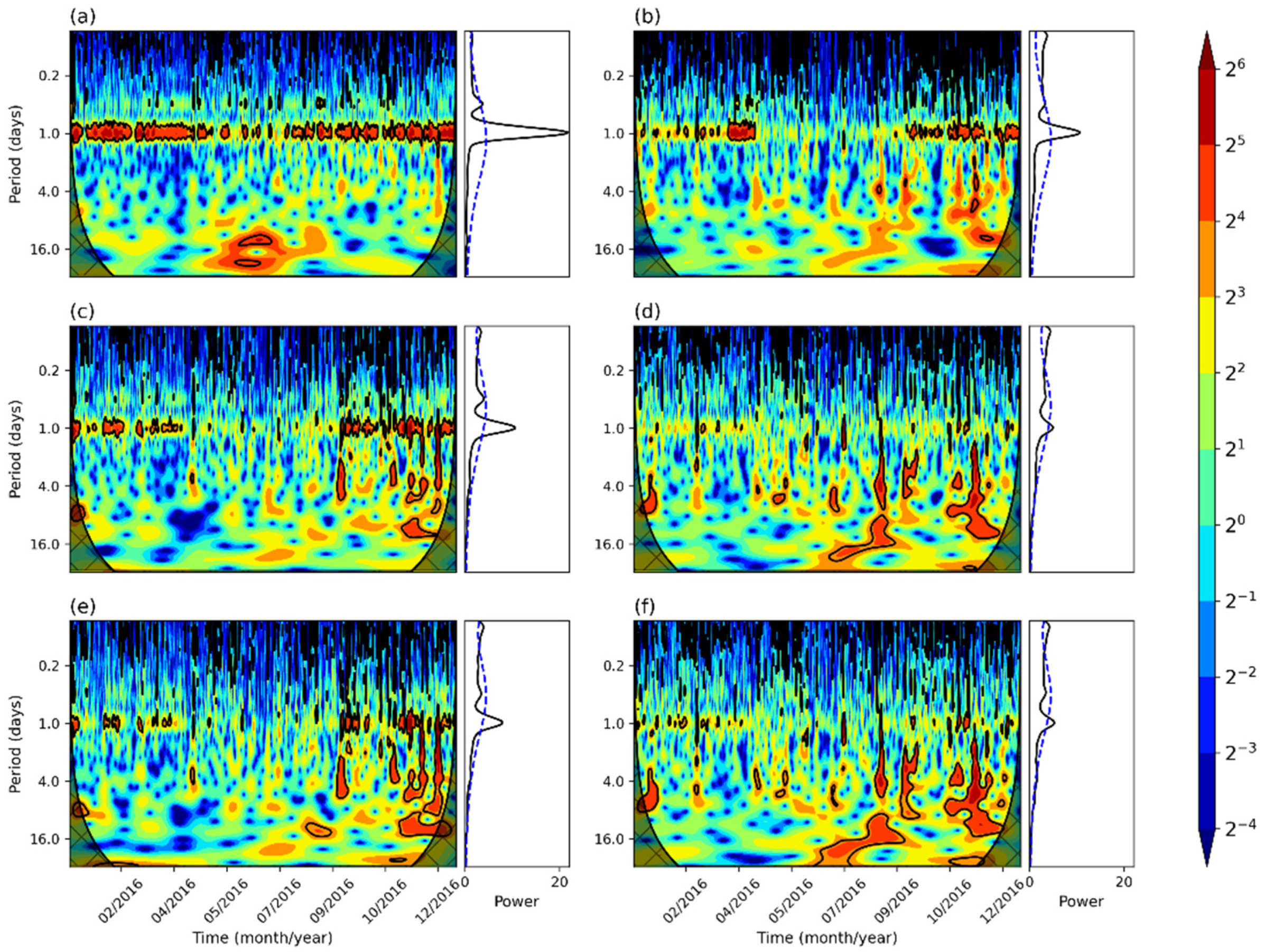
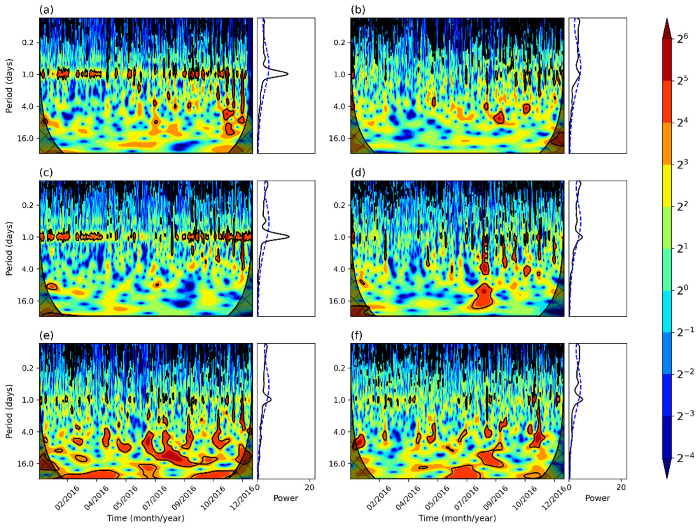
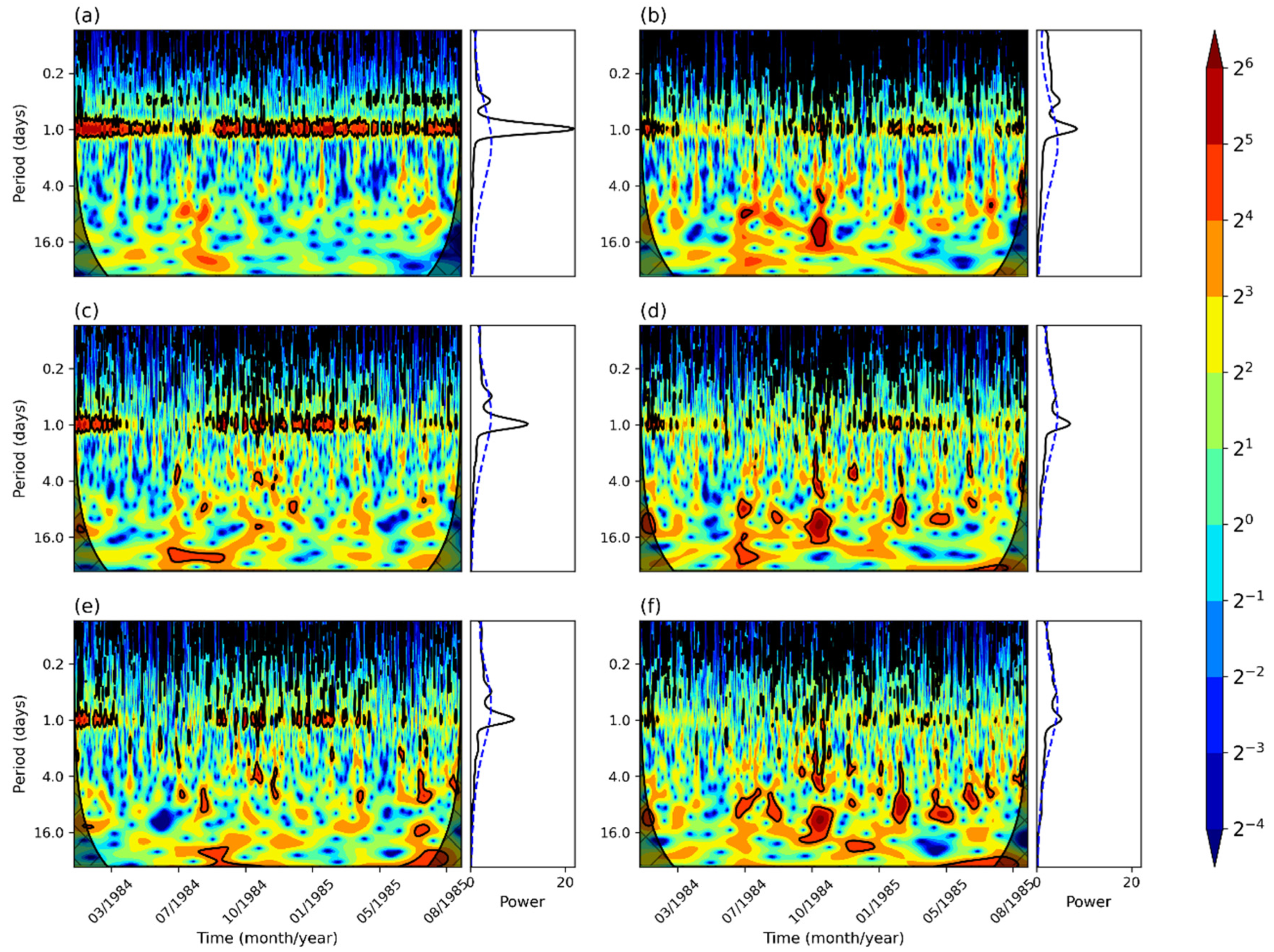
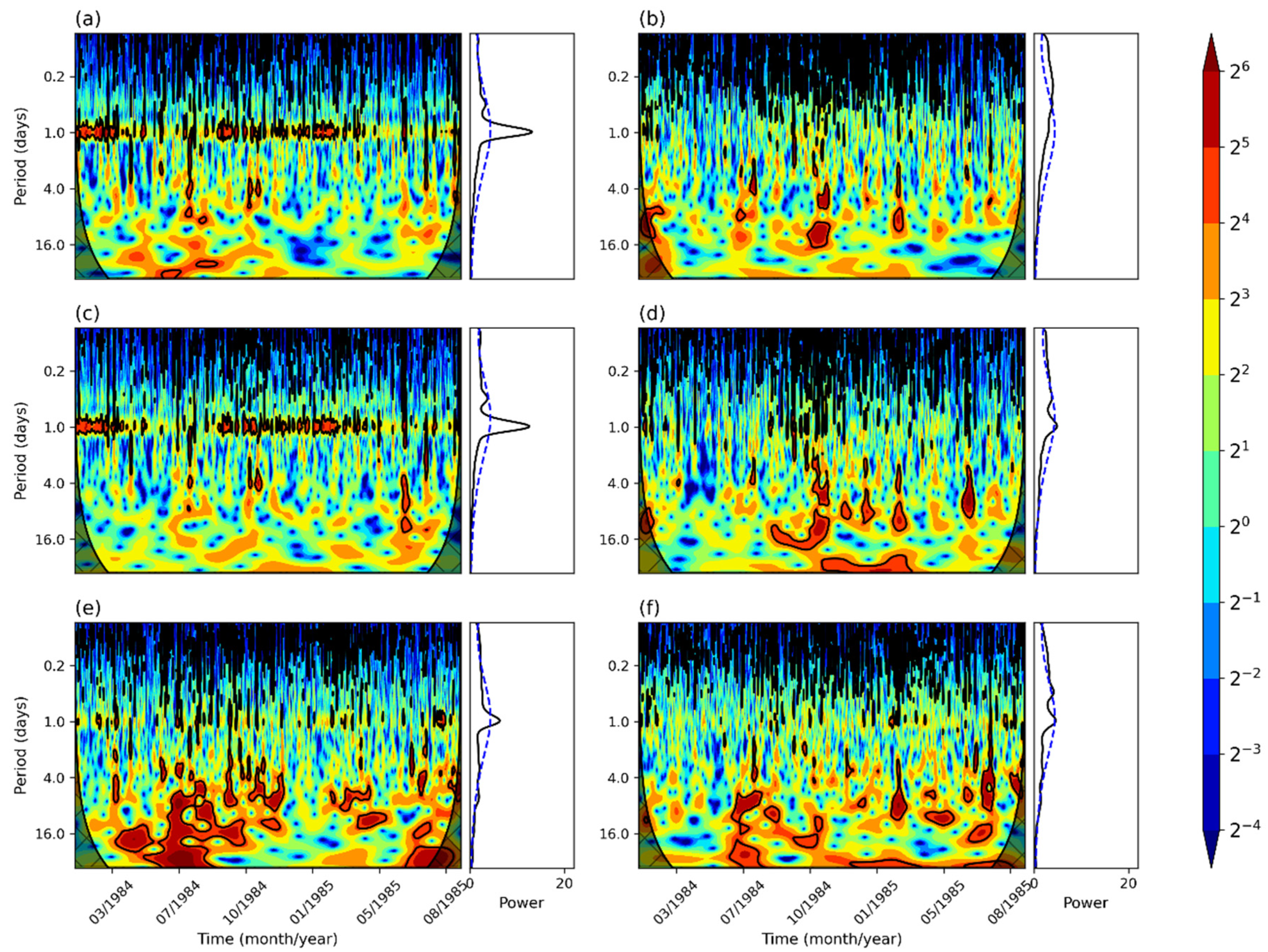
3.2. Identification and Hierarchy of Processes Governing Near-Surface Circulation: Time–Frequency Domain Analysis

As described in Section 2.4, wind data registered in the period from February 1984 to September 1985 and the 2016 full year were used to perform a spectral analysis of the zonal (u) and meridional (v) wind components using wavelet transforms. The two periods were analyzed separately, as two distinct datasets. As the results produced are similar, we chose to analyze the first period, which is a longer period, in this section, while the results for 2016 are provided in Appendix A (Figure A1 and Figure A2).
The wavelet analyses are shown in Figure 13 (for the three levels of tower A) and Figure 14 (for towers B, C and D). The left panels of the figures show the wavelets for meridional wind v, while the right panels correspond to the wavelets for zonal wind u. Each panel shows a shaded area corresponding to the wavelet power spectrum, computed using the Morlet wavelet normalized by the variance of each wind component time series. The thick contour of the shaded area encloses regions of greater than 95% confidence for the red-noise process and the cross-hatched regions indicate the “cone of influence,” in which edge effects become highly important. Moreover, the global wavelet spectrum, calculated by averaging all the local wavelet spectra, is also shown, together with a dashed line indicating the 95% significance level.
The wavelets revealed the occurrence of signals with different frequencies and nonstationary characteristics. The signal with the highest average energy (global spectrum) and statistical significance occurred mostly in the diurnal period (Figure 13 and Figure 14). The only exception was observed for the zonal wind component measured at B-15 m (Figure 13b), in which the diurnal cycle is not evident and there is a high zonal wind direction variability during the day. These results are in line with the findings of the wind roses, which consider a much longer period of analysis and show a pattern of daily change in the direction of the wind with different characteristics among the periods of the day (Figure 5, Figure 6, Figure 7, Figure 8 and Figure 9).
The continuous spectra show a diurnal cycle varying throughout the year, with higher intensity and statistical significance during the austral spring and summer seasons (Figure 13 and Figure 14). These results indicate the same seasonal pattern observed in the boxplot, in which the strongest winds occurred in these seasons and were related to diurnal variability. The diurnal period power is higher for v than for u, which highlights the cross-shore nature of thermally induced circulations (valley/mountain, sea/land and bay) over the CNAAA region. This result reinforces the previous discussion regarding the influence of thermal forcing in the predominant wind directions in the CNAAA.
In addition to the diurnal cycle, the average power shows a semidiurnal cycle with statistical significance. The occurrence of this semidiurnal cycle is associated with the phenomenon of atmospheric thermal tides [87,88]. However, the zonal wind at B-15 m (Figure 14b) and meridional wind at D-15 m (Figure 14e) do not show this secondary peak.
The global and continuous power spectra also reveal a signal with no negligible statistical confidence in the periods between 2 and 6 h, mainly for u (Figure 13 and Figure 14, right-side panels). This timescale variability is possibly associated with the contribution of factors on a local scale. In addition to the thermal forces that induce breeze circulations, the variability of the zonal wind throughout the day would also be modulated on a local scale by the interaction of the flow with the topographical relief [35].
Recalling that tower A was the only tower with sensors installed at different heights (10, 60 and 100 m), the changes in the behavior of the spectra with height could be evaluated. From this, it was observed that, with the increase in height, the power with statistical significance increased for the period between 4 and 16 days, mainly for u (Figure 13b,d,f). This pattern is probably associated with the flow on a synoptic scale, as the passage of transient systems in the study region [37,65]. Furthermore, the power of the diurnal cycle decreased as the altitude of the wind measurements increased. This can be attributed to the measurement point’s distance from the ground surface, where the horizontal temperature gradient forms between the continent and Ilha Grande Bay, which is the driving force of the local circulation of land-sea and bay breezes.
Point D-15 m (Figure 14e,f), which had the highest altitude level, also shows less significant power levels for the diurnal cycle and an increase in power with statistical significance for periods longer than four days. This behavior evidences the influence of the synoptic scale systems over the wind as higher measurements are taken. Moreover, the absence of a continuous spectrum with statistical significance in the diurnal cycle highlights the differences in the measurements obtained at this tower from those obtained at others, as previously shown in the wind frequency distribution (Figure 9).
Therefore, these spectral analyses highlight that, in general, the thermal circulations mainly influence the meridional flow over the region of the CNAAA, on a timescale of 1 day or less. On the other hand, the interactions with the synoptic scale systems are pointed out mainly over the zonal flow, in the period from 4 to 16 days. The most frequent signal in the component u indicates that the modulations from E–W discussed in Section 3.1 may also be related to transient meteorological systems on a synoptic scale, for instance, frontal system, migratory cyclones and SACZ, among others, as already described in previous literature [66,82,86,89,90].

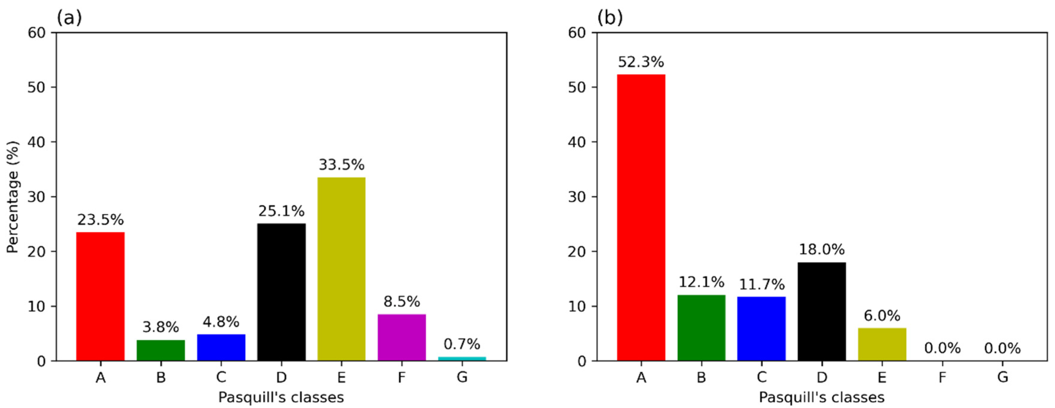
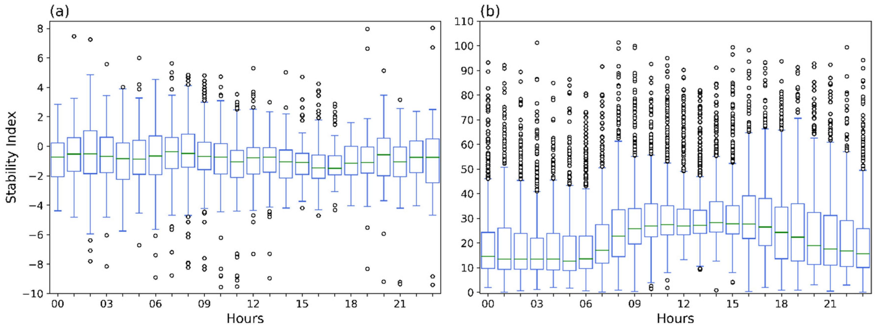
3.3. Characterization of the Local Atmosphere: Stability Analysis

A stability analysis was performed using the measurements from tower A in 2016, correlated to the Pasquill stability classes according to [70], as shown in Table 2. The analysis was based on the vertical temperature gradient (ΔT/ΔZ) and the standard deviation of the wind direction fluctuation at 10 m (σ10). The vertical temperature gradient was computed using measurements of tower A at the altitudes of 10 m and 100 m and the parameter σ10 was directly available from the measurements.
The parameter of static stability (ΔT/ΔZ; Figure 15a) shows higher occurrences of the stability classes D (25.1%) and E (33.5%), which correspond to the predominance in the region of neutral or slightly stable conditions, respectively. This result is in accordance with studies carried out by [37,65,84], in relation to the predominance of stability conditions at the CNAAA. However, a third predominant stability class, A, was also identified, which corresponds to highly unstable conditions; this result differs from previous studies. This increase in the observation of unstable conditions in 2016, compared to previous studies, is possibly associated with changes in the land use around tower A. This would be due to the ongoing construction of the Angra III power plant, which is directly correlated with greater surface heating.
The hourly distribution of the static stability parameter is shown in the boxplots in Figure 16a. The median of the data is variable throughout the day, lightly decreases during the morning and reaches lower values in the afternoon. It is also noteworthy that the boxplots for the times of greatest heating (3 p.m. and 4 p.m.) show the lowest interquartile range, that is, the lowest values of the 3rd quartile of the entire day cycle (Figure 16a). This pattern indicates that daytime heating induces a lower number of stable situations in the afternoon.
The standard deviation of the wind direction fluctuation (Figure 15b) provides a panorama of stability that is different from that measured by the vertical temperature gradient. From this parameter, the most frequent Pasquill stability class was A (52.3%), followed by the D, B, C and E classes (Figure 15b). In addition, the hourly distribution of this parameter evidenced a daily cycle (Figure 16b).
Throughout the evening, the boxplots had an asymmetric distribution with the lowest median values (Figure 16b). During this period of the day, approximately half of the records corresponded to neutral or stable conditions. After the early morning, it appears that the median reached the highest values, with its maximum peaking throughout the afternoon, during which more than half of the records were greater than 22.5°. Thus, according to the categorization of the parameter σ10 according to [70], the daily cycle observed in the boxplot indicates that there was greater mechanical turbulence in the afternoon, when the surface flux is commonly forced by the circulation of the sea breeze. According to [65], greater mechanical turbulence within the atmospheric boundary layer is directly related to the maximum height of the breeze spread. The evaluation of the conditions of stability of the local atmosphere, both by thermodynamic and mechanical mechanisms (Figure 16), reveal that, in the afternoon, atmospheric conditions contribute to increase the pollutants dispersion.

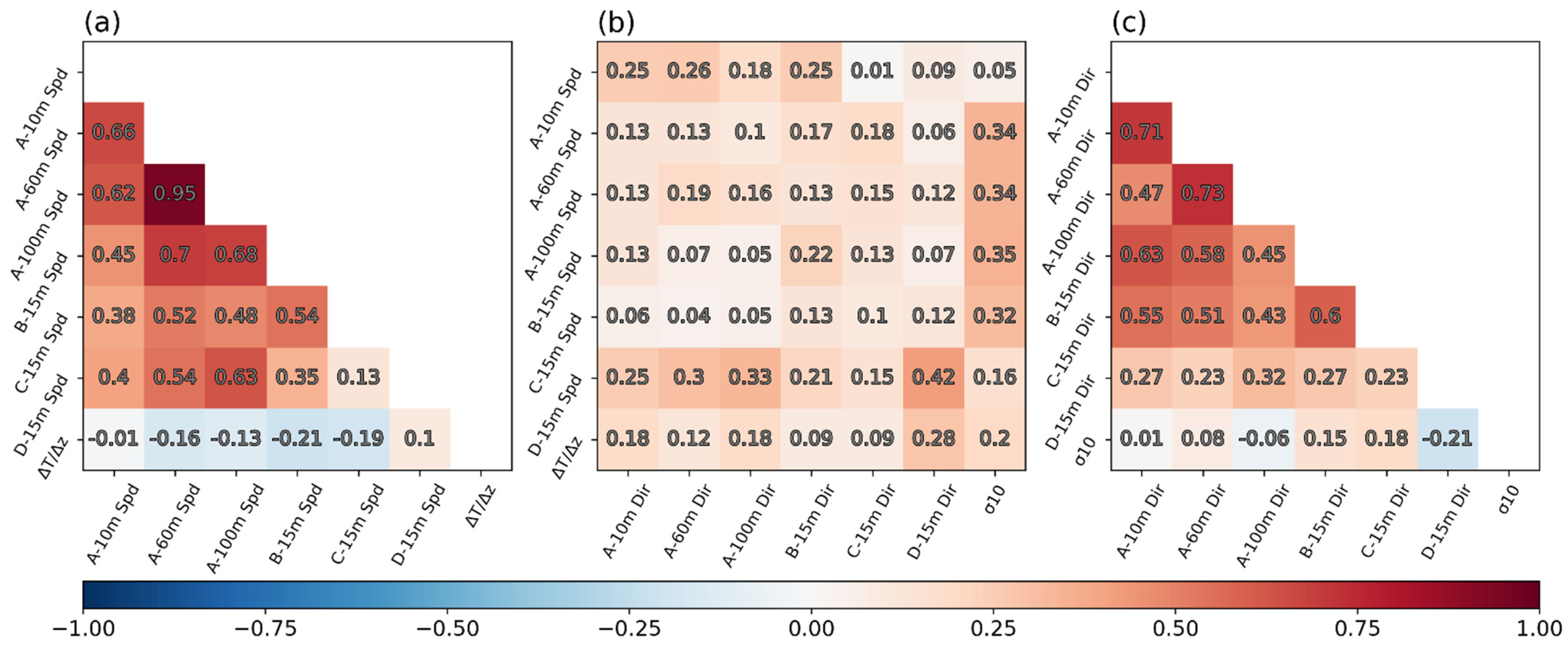
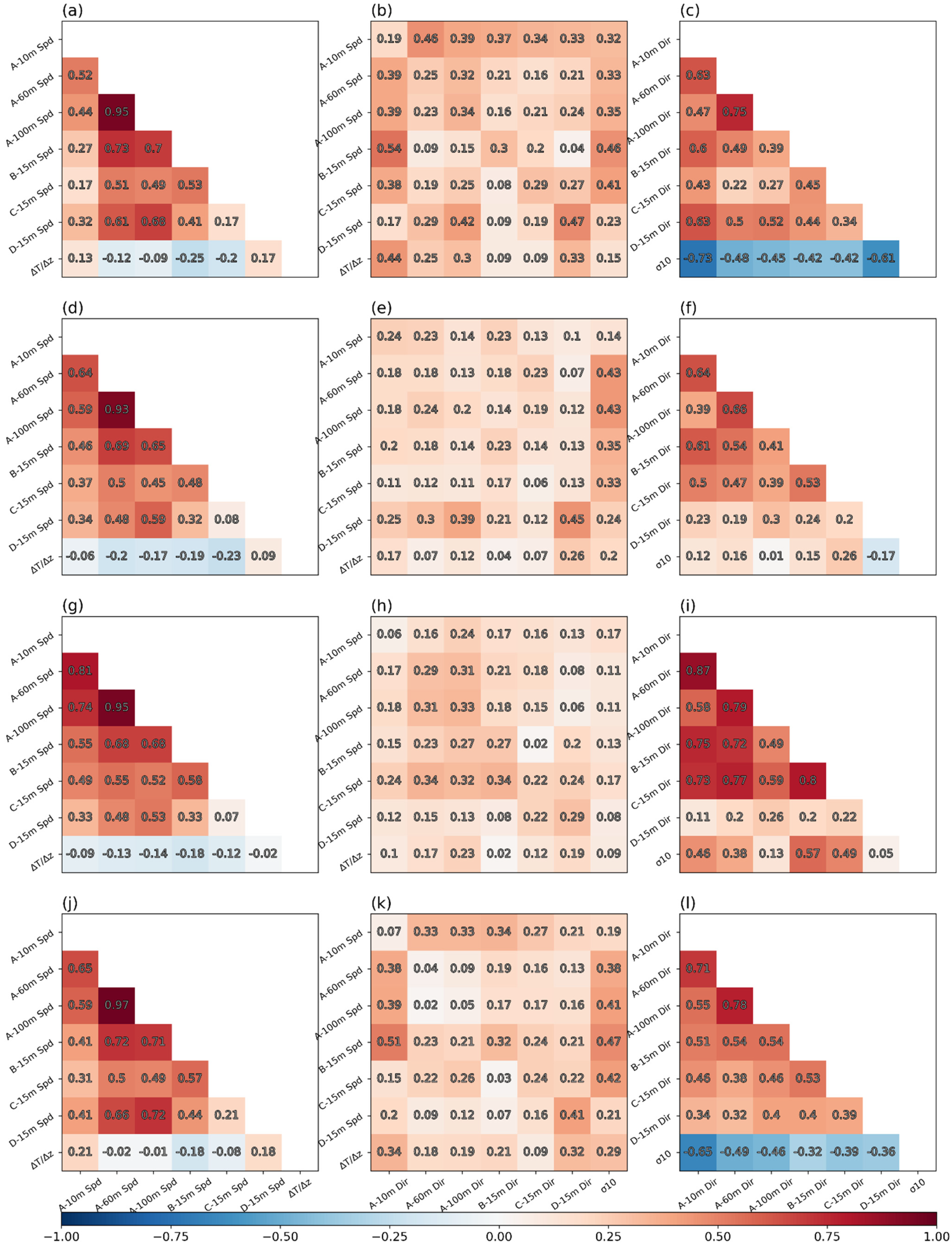
3.4. Wind and Stability Data of the Local Atmosphere: Correlation Analysis

The analysis of the atmospheric stability class, its variation with the daily cycle and seasonality are crucial in nuclear installation safety protocols. This information is an indirect but easily obtainable measure of the dispersion capacity in the atmospheric boundary layer of NPP installation sites [70].
Based on this concept, [37] presented an analysis based on qualitative criteria such as frequency graphs that revealed a close relationship between the wind regime (direction and intensity) and the atmospheric stability regime in the CNAAA region. In the current study, this analysis incorporates the quantification of this relationship using statistical indices. This information may be used, in the future, to assess computational atmospheric modeling systems, such as WRF, and their ability to represent this behavior by assisting in the realistic estimate of pollutant dispersion in the atmosphere in case of a nuclear accident with radionuclide release.
Given that wind direction is a circular variable, it is necessary to take special care in calculating the correlation coefficient between the circular–linear variable and circular–circular variable using well-established criteria in the scientific literature (circular statistic area of knowledge). The studies cited show that the use of the circular correlation index, which is appropriate for assessing the degree of association between circular variables (such as wind direction) and linear variables (such as wind intensity and stability class), goes beyond a mathematical formula, with significant studies available in the open scientific literature for several areas of interest [78,91,92,93].
Figure 17 illustrates the correlation matrix between the wind and atmospheric stability data at the six measurement points distributed around the CNAAA. In general, most of the calculated correlations were positive. The static stability parameter showed small correlations (<|0.2|) with respect to the wind data of the towers and it was negatively correlated with the stability parameter σ10. The variable σ10 showed correlations greater than 0.3 with the wind speed at A-60 m, A-100 m, B-15 m and C-15 m. There was also a high correlation between the wind data measured in the towers.
An analysis of the diurnal cycle of the stability parameters showed negative correlations between the variable σ10 and the variation of wind directions during the evening and early morning periods, during which there were higher registers of stable conditions (Figure 18). In the morning and afternoon periods, when the σ10 data mostly corresponded to unstable situations, the variable was positively correlated with the wind directions of the CNAAA towers. The correlations of σ10 with the wind data were stronger than the correlations of the parameter ΔT/Δz with the same data throughout the day cycle (Figure 18). This result is possibly due to σ10 being directly related to wind variability, while ΔT/Δz considers only the vertical variation of temperature in its formulation.
The correlation between the wind intensity at A-60 m and A-100 m was 0.96 and the correlation between the wind direction data from these two points was 0.73 (Figure 17). The correlation between the A-60 m and A-100 m data remained high in the four correlation matrices decomposed by the daily cycle, with a correlation above 0.93 for the intensity and above 0.66 for the direction (Figure 18). A very similar result of the wind distribution between these two points was also observed in the wind frequency distribution graphs (Figure 5 and Figure 6). This similar correlation reinforces that the flow at these two points was likely induced by the same driving forces as those which influenced all towers throughout nearly the entire analyzed period.
The wind directions measured at A-10 m, A-60 m, A-100 m, B-15 m and C-15 m have correlations between 43% and 73%, again indicating a certain degree of similarity between these four tower sites (Figure 17). However, D-15 m differs notably from the others in terms of the daytime cycles of the wind direction and intensity. Consequently, the correlation between the direction of the point was less than 32% at most of the other points (Figure 17). In relation to the correlation matrices corresponding to each period of the day (Figure 18), it is noteworthy that there are no large differences in the magnitude values of most highly correlated variables. However, it may be noted that the highest values of positive correlation between the wind data occur, in general, in the afternoon period, in which the predominant winds are attributed to the sea breeze at all points.

3.5. Integrated Analysis to Identify the Main Forcing, System and Process to CNAAA’s Region Modeling (Atmospheric and Radionuclide Dispersion Models)

The wind rose graphics, time–frequency analysis classical and circular statistics, provide a valuable integrated methodological approach for identifying the main mechanisms of atmospheric transport in coastal regions with complex topography. This analysis allows the identification of the primary forcing and meteorological systems acting over a non-homogeneous region, as well as some mechanisms influencing the circulation in an independent or coupled manner. A better understanding of these processes and meteorological systems is critical because similar conditions are observed around the world in regions where other NPPs are installed. The knowledge gained via this investigation may be utilized to create safety protocols for areas with physiographic features similar to those present in the CNAAA’s area. Furthermore, this sort of analysis should be carried out on a regular basis to ensure that computational systems for atmospheric and radionuclide dispersion modeling are properly configured.
Table 4 shows a summary of the wind regime in each one of the CNAAA towers, as well as the spatio-temporal meteorological effects acting over the towers and the processes induced by these scales.
The 20-year wind climatology clearly shows the complexity of the phenomena acting in the CNAAA region. The integrated analyses of wind roses, boxplots and wavelets allow us to assess the predominance of the wind direction, and the calm and high-intensity winds, as well as identifying the characteristic timescales of synoptic, local breezes and tidal systems. As discussed in Section 3.2, the statistically significant wavelet power spectrum of 4–16 days increased as measurement height increased, mainly for zonal wind. This pattern clearly indicates that synoptic systems have an impact on winds in these higher periods. Synoptic influences over winds can be regarded as affecting directly both the towers D-15 m and A-100 m, since tower D-15 m showed greater power spectra in the aforementioned periods and it has a higher correlation with tower A-100 m measurements. Furthermore, the strong correlation between the wind speed (linear–linear) and direction (circular–circular) of tower A-60 m and towers A-10 m and A-100 m indicates that this is a height where surface and local circulation effects begin to diminish and synoptic effects begin to contribute to the resultant wind.
The interaction of synoptic and mesoscale systems, such as land channeling and its blocking and recirculation effect, is known to be influenced by the physiographic structure of the region. In addition, the spatial (both vertically and horizontally) and temporal diversity of the wind behavior and stability class is associated with the breeze systems, as well as with the generation and consumption of thermal and mechanical turbulence in the atmospheric boundary layer and with the insolation daily cycle, besides the annual seasonality. Therefore, a better understanding of these processes, systems and phenomena aids in the selection and definition of the region’s atmospheric modeling system configuration. The presence of calm winds, especially in the tower-A region (at 60 m and 100 m) between the evening and morning, emphasizes the need of adopting suitable pollutant dispersion models in that location, as certain dispersion models are ineffective in calm wind circumstances [94,95,96,97]. Furthermore, the occurrence of statically stable stability classes suggests that the CNAAA area is less capable of turbulent diffusion. This condition has a direct impact on radionuclide releases that occur by accident. In this regard, an emergency plan is provided in the next section to emphasize the significance of this integrated analysis.
Following the analysis, the main features that the atmospheric and dispersion of pollutants modeling system should have for an adequate depiction of the CNAAA region were identified as follows: complex terrain transport, non-homogeneous boundary layer, calm wind regime, winds above 17m/s (at A-100 m, B-15 m, C15 m and D-15 m), static stability classes (mainly D and E), thermal and dynamic internal boundary layer formation and katabatic and anabatic winds. Based on the spatial diversity identified with the aid of observational data from CNAA towers, the presented analysis can also anticipate some important configurations that an atmospheric and radionuclide dispersion modeling system should have to represent the various forcing and mechanisms in coastal regions with mountain ranges. The modeling features based on s prevalently local time–space scale observed at towers A-10 m, A-60 m, B-15 m and C-15 m are the following:
  • Initial and boundary conditions: high resolution databases of topography, land use land cover (LULC) categories and coastline and time-varying sea surface temperature (SST).
  • Domain: vertical (<50 m) and horizontal high resolution (<1 km) and number of points.
  • Physical parametrization: soil, surface and boundary layer, longwave and shortwave radiation and microphysics; Large Eddy simulation (LES).
  • Other: nested grids, observational data assimilation, nonhydrostatic and hybrid sigma-pressure vertical coordinate.
The modeling features based on a prevalently synoptic time–space scale observed at towers D-15 m and A-100 m are the following:
  • Initial and boundary conditions: global atmospheric model, high resolution databases of topography and LULC.
  • Physical parametrization: boundary layer, horizontal diffusion, longwave and shortwave radiation and microphysics.
  • Other: nested grids, observational data assimilation, nonhydrostatic and hybrid sigma-pressure vertical coordinate.
In order to evaluate the model results, the nearest grid point is generally used to extract the model information to be compared to the observations [98]. Care must be taken when selecting the grid point position to avoid representativeness errors. The nearest grid point may be at a different height [26] and in a different location of the terrain feature than in reality since the model orography is smoothed [98]. It is also a concern in coastal regions, because the nearest model grid point can be located over water, while the surface-based observation is located over land and vice versa. It reinforces the necessity of the use of a high-resolution topography database, as well as a vertical and horizontal grid.

3.6. Integrated Environmental Analysis for Emergency Planning in the CNAAA’s Area

Considering the main safety objective of nuclear installations, namely, to ensure that the radiological impact on the population and the environment during the operational phase and in accidental conditions is within the levels prescribed by the regulatory authority, local characteristics that may affect emergency response conditions must be carefully studied. Hazards that could affect the safety of nuclear facilities must be properly considered, particularly in site selection and assessment, design of new facilities (especially during site selection and assessment), design of new installations and operational phases of existing installations [20]. Furthermore, evacuation routes and access to areas of influence are critical factors in emergency planning. As a result, the geobiophysiographic aspects of these areas (geographical, geological, geo-morphological, hydrological and meteorological elements) must be assessed [57,99].
The characteristics of the CNAAA’s surroundings demonstrate the region’s geobiophysiographic and socio-environmental complexity, as well as its vulnerabilities, which serve as the primary bottlenecks in the context of local emergency planning (Figure 19). The predominant wind directions, the rainfall regime, the occurrence of flooding and landslides (2007–2019) and the population quantity are all factors that contribute to the complexity of implementing planning actions during the accident-response phase.
The prevailing winds in the region are N (night and dawn) and SW (morning and afternoon), which determine the primary escape routes in the process of evacuating the population in the event of an accident (Table 4). Rainfall with monthly averages above 70 mm occurs approximately 158 days per year, with greater intensity between October and April and with January presenting averages of 276.4 mm [65,100]. This region has the highest rainfall rate in the state of Rio de Janeiro, causing flooding in drainage and landslide areas that cover densely populated areas.
In terms of nuclear emergency evacuation, in general, this process involves significant populations and the risks of radiation exposure in areas with limited road capacity, a similar aspect in the CNAAA’s area of influence, where BR-101 is the only axis of mobility on a local and regional scale. In this sense, when considering the highway evacuation, the N winds indicate the SW and NE directions as an escape route and, when the wind is from the SW, the SW direction. Considering the elements of rain, especially in periods with greater rainfall and landslides, with medium and high susceptibilities throughout the region, these are aspects that jointly limit evacuation actions along the BR-101 highway, determining population sheltering as the primary decision-making process, whether due to punctual flooding in stretches located in areas of higher population density, as well as through landslides that can block access by road [53,54].
Other relevant aspects that are part of the aforementioned problems include the following, among others [44]: the increase in population flow, from seasonal variations (floating population) increased by tourist activity and/or exceptional demographic concentrations (popular festivals and regional or local events); road traffic, with traffic jams in high season and long holidays, intensified by regional tourism; traffic on the BR-101 highway, with poor paving, signaling and lighting conditions and slopes between 5° and 30°; a lack of electricity during emergencies, particularly in areas with a higher population density and difficult access to the streets (narrow streets, pavements and slopes).
The integrated analysis of these aspects represents a significant subsidy that can support the reduction in risks, prevention and mitigation of the consequences of accidental events in the area of influence of the CNAAA and in the nuclear sector [101], in regions with similarities and especially the preparation of emergency responses, which is one of the objectives of emergency planning [102], in addition to ensuring the functioning of the emergency response system [103].

4. Conclusions

In this study, advances were made in the characterization of wind and stability regimes in the CNAAA region based on the application of statistical modeling combined strategies. The use of data mining tools applied in the time and frequency domains is promising for providing relevant information for the identification and hierarchization of thermally and mechanically driving forcing in coastal and complex topography regions, with the aim of informing the design of safety protocols and accident mitigation plans in nuclear installations.
The methodological procedure of the scientific study, in addition to supporting the nuclear safety protocols, presents a universalist character and can be extended to other regions of the world with potential capacity for nuclear centrals, contributing to revise safety protocols of the NPPs already in operation. The importance of the study for the adequacy and skill evaluation of computational modeling systems for atmospheric dispersion of pollutants such as radionuclide and conventional contaminants can be also highlighted, in order that such systems are used as tools for environmental planning and managing of nuclear operations, particularly those located in regions over mountainous and coastal environments with a heterogeneous atmospheric boundary layer.
The predominant wind and stability regime around the nuclear complex were attributed to the combination of thermally induced systems by heterogeneous terrain, mechanically driven forcing by topography and the action of the synoptic systems. The contribution of different spatial and temporal scales in the wind direction was reinforced by the analysis of wavelet spectra with statistical significance in the time scales from the microscale (hours) to the synoptic scale (days).
Wind intensity between 1 and 3 m·s−1 makes up most of the records for the CNAAA monitoring network. The tower points A-60 m and A-100 m presented the highest percentage of calm regime, at approximately 12.58%. The highest wind intensity records correspond to 25–30 m·s−1 (80–108 km/h), mainly in the afternoon. A seasonal pattern could be observed that modulated the highest wind intensities, in which the strongest wind intensity occurred in the austral spring and summer.
The static stability analysis indicated the following higher Pasquill stability classes: E (slightly stable), D (neutral) and A (strongly unstable). The standard deviation parameter of wind direction fluctuation shows the predominance of class A, followed by classes D, B, C and E. This finding differs from previous research by [84] and [37]. Given that the wavelet analysis for 1984–1985 and 2016 are very similar, the difference appears to be unrelated to changes in the region’s land use and land cover.
The analysis of the wavelet spectra revealed the occurrence of signals with different temporal scales and nonstationary characteristics. The signal with the highest average power and statistical significance occurred in the daytime cycle during the austral spring and summer because of the thermally induced circulation of the valley/mountain and sea/land systems. The second highest average power occurred on the semidiurnal scale, which can be related to the phenomenon of the atmospheric thermal tide. Signs that occurred in periods from 2 to 6 h were also observed, indicating the possible influence of the atmospheric flow on the orography. Another wind regime pattern occurred at ~4–20 days, associated with the synoptic scale system and active in the region as a frontal system, migratory cyclones and the SACZ.
We also made use of an emerging area of knowledge, called circular statistics, for the identification of the relationship of circular variables such as wind direction over physical behaviors in the atmospheric boundary layer. The correlation matrix analysis indicated a higher similarity in the wind and temperature records at A-60 m, A-100 m, B-15 m and C-15 m. The tower point D-15 m represents the lowest correlation for the CNAAA, as compared to the other points, which reinforces the variability of the flow at this location in relation to the other monitoring network sites.
The main features that the atmospheric and dispersion of pollutants modeling system should have for an adequate depiction of the CNAAA region were identified as complex terrain transport, non-homogeneous boundary layer, calm wind regime, winds above 17 m/s (at A-100 m, B-15 m, C15 m and D-15 m), static stability classes (mainly D and E), thermal and dynamic internal boundary layer formation and katabatic and anabatic winds. The analysis presented here can also anticipate some important configurations that an atmospheric and radionuclide dispersion modeling system should have in order to represent the boundary layer flow in coastal and mountain regions.
The main bottlenecks that the CNAAA region presents, its complexities and vulnerabilities, and the importance to perform detailed analysis to elaborate local emergency planning, are highlighted in this study. By using a geographic information system platform, it is demonstrated the need to establish escape routes and places to shelter the population.

Author Contributions

Conceptualization, (L.d.F.R.J., L.C.G.P. and L.P.d.F.A.); methodology, (J.F.d.O.J., I.C.D.V.D., C.S. and W.C.M.d.F.); software, (L.d.F.R.J., I.C.D.V.D., C.S. and W.C.M.d.F.); validation, (J.F.d.O.J., J.S.P.G. and P.F.L.H.F.); formal analysis, (L.d.F.R.J., L.C.G.P., E.M., L.P.d.F.A., J.F.d.O.J., I.C.D.V.D., C.S. and W.C.M.d.F.); investigation, (L.d.F.R.J., L.C.G.P., J.F.d.O.J., I.C.D.V.D.); resources, (L.C.G.P., L.P.d.F.A. and L.L.); data curation, (L.C.G.P., L.P.d.F.A., J.S.P.G., P.F.L.H.F. and L.L.); writing—original draft preparation, (L.d.F.R.J., L.C.G.P., J.F.d.O.J., I.C.D.V.D., C.S. and W.C.M.d.F.); writing—review and editing, (L.d.F.R.J., L.C.G.P., J.F.d.O.J., I.C.D.V.D., C.S. and W.C.M.d.F.); visualization, (E.M., J.S.P.G., P.F.L.H.F. and L.L.); supervision, (L.C.G.P. and L.P.d.F.A.); project administration, (L.C.G.P. and L.P.d.F.A.); funding acquisition, (L.C.G.P., L.P.d.F.A., J.S.P.G., P.F.L.H.F. and L.L.). All authors have read and agreed to the published version of the manuscript.

Funding

This research was funded by Brazilian Nuclear Energy Commission (CNEN) grant number CNEN 1/2018, and Brazilian National Council for Scientific and Technological Development (CNPq) grant number 313625/2018-2.

Institutional Review Board Statement

Not applicable.

Informed Consent Statement

Not applicable.

Data Availability Statement

Not applicable.

Acknowledgments

The authors are grateful to the agencies CAPES (Coordenação de Aperfeiçoamento de Pessoal de Nível Superior), CNPq (Conselho Nacional de Desenvolvimento Científico e Tecnológico) and Brazilian Nuclear Energy Commission (CNEN). Larissa Jacinto was supported by the Master’s scholarship funded by the Brazilian Nuclear Energy Commission (CNEN). We are grateful to the Eletrobras Eletronuclear institution for providing the meteorological data for the tower. We also thank Evgeniya Predybaylo, who developed the Python wavelet software based on Torrence and Compo (1998) available at URL: http://atoc.colorado.edu/research/wavelets/. Accessed on 5 October 2021.

Conflicts of Interest

The authors declare no conflict of interest.

Appendix A

Figure A1. Wavelet transform and global wavelet spectrum for wind component (left) and wind component (right) at (a,b) A-10 m, (c,d) A-60 m. and (e,f) A-100 m. The black contour at the wavelet transform and the dashed line at the global wavelet spectrum limit the 5% significance level. The cross-hatched region is the cone of influence.
Atmosphere 12 01321 g0a1
Figure A2. Wavelet transform and global wavelet spectrum for wind component (left) and wind component (right) at (a,b) B-15 m, (c,d) C-15 m. and (e,f) D-15 m. The black contour at the wavelet transform and the dashed line at the global wavelet spectrum limit the 5% significance level. The cross-hatched region is the cone of influence.
Atmosphere 12 01321 g0a2

References

  1. Bradshaw, A.M.; Hamacher, T.; Fischer, U. Is Nuclear Fusion a Sustainable Energy Form? Fusion Eng. Des. 2011, 86, 2770–2773. [Google Scholar] [CrossRef] [Green Version]
  2. Bornschein, B.; Day, C.; Demange, D.; Pinna, T. Tritium Management and Safety Issues in ITER and DEMO Breeding Blankets. Fusion Eng. Des. 2013, 88, 466–471. [Google Scholar] [CrossRef]
  3. International Atomic Energy Agency, (IAEA). Nuclear Share of Electricity Generation in 2020. Available online: https://pris.iaea.org/PRIS/WorldStatistics/NuclearShareofElectricityGeneration.aspx (accessed on 21 June 2021).
  4. Molinier, L.; Combescure, C.; Chouaid, C.; Daurès, J.-P.; Housset, B.; Fabre, D.; Grand, A.; Vergnenègre, A. Cost of Lung Cancer: A Methodological Review. PharmacoEconomics 2006, 24, 651–659. [Google Scholar] [CrossRef]
  5. Iwata, H.; Okada, K.; Samreth, S. Empirical Study on the Environmental Kuznets Curve for CO2 in France: The Role of Nuclear Energy. Energy Policy 2010, 38, 4057–4063. [Google Scholar] [CrossRef] [Green Version]
  6. Intergovernmental Panels on Climate Change, (IPCC). Renewable Energy Sources and Climate Change Mitigation: Special Report of the Intergovernmental Panel on Climate Change; Ottmar, E., Ramón, P.-M., Youba, S., Kristin, S., Susanne, K., Timm, Z., Patrick, E., Gerrit, H., Steffen, S., von Christoph, S., Eds.; Patrick Matschoss: Cambridge, UK, 2012; ISBN 978-1-107-60710-1. [Google Scholar]
  7. Visschers, V.H.M.; Keller, C.; Siegrist, M. Climate Change Benefits and Energy Supply Benefits as Determinants of Acceptance of Nuclear Power Stations: Investigating an Explanatory Model. Energy Policy 2011, 39, 3621–3629. [Google Scholar] [CrossRef]
  8. Baek, J. A Panel Cointegration Analysis of CO2 Emissions, Nuclear Energy and Income in Major Nuclear Generating Countries. Appl. Energy 2015, 145, 133–138. [Google Scholar] [CrossRef]
  9. Oliveira, S.S.B.; Santos, D.; Cardoso, D.L.; Ruzene, D.S.; Silva, D.P.; do Amaral, G.R. Energia Nuclear: Vantagens e Desvantagens. An. VIII SIMPROD 2016, 3, 362–368. [Google Scholar]
  10. Rashad, S.M.; Hammad, F.H. Nuclear Power and the Environment: Comparative Assessment of Environmental and Health Impacts of Electricity-Generating Systems. Appl. Energy 2000, 65, 211–229. [Google Scholar] [CrossRef]
  11. Hore-Lacy, I. Nuclear Energy in the 21st Century; World Nuclear University Press: London, UK, 2007; ISBN 978-0-12-373622-2. [Google Scholar]
  12. Menyah, K.; Wolde-Rufael, Y. CO2 Emissions, Nuclear Energy, Renewable Energy and Economic Growth in the US. Energy Policy 2010, 38, 2911–2915. [Google Scholar] [CrossRef]
  13. Price, R.; Blaise, J.R. NEA Updates, NEA News 2002; The Nuclear Energy Agency: Paris, France, 2002; pp. 10–13. [Google Scholar]
  14. British Petroleum, (BP). BP Statistical Review of World Energy 2019; British Petroleum (BP): London, UK, 2019; pp. 1–64. [Google Scholar]
  15. de Saraiva, G.J.P. Energia Nuclear No Brasil: Fatores Internos e Pressões Externas; Cadernos de Estudos Estratégicos, Centro de Estudos Estratégicos, Escola Superior de Guerra: Rio de Janeiro, Brazil, 2007; ISBN 9771808947002. [Google Scholar]
  16. Gioia, A. Nuclear Accidents and International Law. In International Disaster Response Law; de Guttry, A., Gestri, M., Venturini, G., Eds.; TMC Asser Press: The Hague, The Netherlands, 2012; pp. 85–102. ISBN 978-90-6704-881-1. [Google Scholar]
  17. Empresa de Pesquisa Energética, (EPE). Potencial dos Recursos Energéticos no Horizonte 2050; Recursos Energéticos; Empresa de Pesquisa Energética (EPE): Rio de Janeiro, Brazil; Ministério de Minas e Energia (MME): Rio de Janeiro, Brazil, 2018; p. 186. [Google Scholar]
  18. International Atomic Energy Agency, (IAEA). Nuclear Technology Review 2012; International Atomic Energy Agency (IAEA): Vienna, Austria, 2012; p. 182. [Google Scholar]
  19. Empresa de Pesquisa Energética, (EPE). Plano Nacional de Energia 2030; Projeções; Empresa de Pesquisa Energética (EPE): Rio de Janeiro, Brazil; Ministério de Minas e Energia (MME): Rio de Janeiro, Brazil, 2007; pp. 1–372. [Google Scholar]
  20. International Atomic Energy Agency, (IAEA). Meteorological and Hydrological Hazards in Site Evaluation for Nuclear Installations: Safety Guide; IAEA Safety Standards Series No. SSG-18; International Atomic Energy Agency (IAEA): Vienna, Austria, 2011; ISBN 978-92-0-115210-7. [Google Scholar]
  21. World Meteorological Organization (WMO). Guide to Instruments and Methods of Observation; World Meteorological Organization: Geneva, Switzerland, 2018; ISBN 978-92-63-10008-5. [Google Scholar]
  22. Calpini, B.; Ruffieux, D.; Bettems, J.-M.; Hug, C.; Huguenin, P.; Isaak, H.-P.; Kaufmann, P.; Maier, O.; Steiner, P. Ground-Based Remote Sensing Profiling and Numerical Weather Prediction Model to Manage Nuclear Power Plants Meteorological Surveillance in Switzerland. Atmos. Meas. Tech. 2011, 4, 1617–1625. [Google Scholar] [CrossRef] [Green Version]
  23. Krivec, T.; Kocijan, J.; Perne, M.; Grašic, B.; Božnar, M.Z.; Mlakar, P. Data-Driven Method for the Improving Forecasts of Local Weather Dynamics. Eng. Appl. Artif. Intell. 2021, 105, 104423. [Google Scholar] [CrossRef]
  24. Lehner, M.; Rotach, M. Current Challenges in Understanding and Predicting Transport and Exchange in the Atmosphere over Mountainous Terrain. Atmosphere 2018, 9, 276. [Google Scholar] [CrossRef] [Green Version]
  25. Paiva, L.M.S.; Bodstein, G.C.R.; Pimentel, L.C.G. Influence of High-Resolution Surface Databases on the Modeling of Local Atmospheric Circulation Systems. Geosci. Model Dev. 2014, 7, 1641–1659. [Google Scholar] [CrossRef] [Green Version]
  26. Warner, T.T. Numerical Weather and Climate Prediction; Amsterdam University Press: Amsterdam, The Netherlands, 2009; p. 21. [Google Scholar]
  27. Suarez, A.; Stauffer, D.R.; Gaudet, B.J. Wavelet-Based Methodology for the Verification of Stochastic Submeso and Meso-Gamma Fluctuations. Mon. Weather Rev. 2015, 143, 4220–4235. [Google Scholar] [CrossRef]
  28. Mattar, C.; Borvarán, D. Offshore Wind Power Simulation by Using WRF in the Central Coast of Chile. Renew. Energy 2016, 94, 22–31. [Google Scholar] [CrossRef]
  29. Olson, J.B.; Kenyon, J.S.; Djalalova, I.; Bianco, L.; Turner, D.D.; Pichugina, Y.; Choukulkar, A.; Toy, M.D.; Brown, J.M.; Angevine, W.M.; et al. Improving Wind Energy Forecasting through Numerical Weather Prediction Model Development. Bull. Am. Meteorol. Soc. 2019, 100, 2201–2220. [Google Scholar] [CrossRef]
  30. Bou-Zeid, E.; Anderson, W.; Katul, G.G.; Mahrt, L. The Persistent Challenge of Surface Heterogeneity in Boundary-Layer Meteorology: A Review. Bound.-Layer Meteorol. 2020, 177, 227–245. [Google Scholar] [CrossRef]
  31. Edwards, J.M.; Beljaars, A.C.M.; Holtslag, A.A.M.; Lock, A.P. Representation of Boundary-Layer Processes in Numerical Weather Prediction and Climate Models. Bound.-Layer Meteorol. 2020, 177, 511–539. [Google Scholar] [CrossRef]
  32. International Atomic Energy Agency, (IAEA). Nuclear Technology Review 2020; International Atomic Energy Agency (IAEA): Vienna, Austria, 2020; p. 77. [Google Scholar]
  33. Silva, C.; Landau, L.; Claudio Gomes Pimentel, L.; Fernando Lavalle Heilbron Filho, P. GIS as a Decision Support Tool in the Area of Influence of the Nuclear Complex Angra Dos Reis, Brazil. JGIS 2013, 5, 13–23. [Google Scholar] [CrossRef] [Green Version]
  34. Whiteman, C.D.; Doran, J.C. The Relationship between Overlying Synoptic-Scale Flows and Winds within a Valley. J. Appl. Meteor. Climatol. 1993, 32, 1669–1682. [Google Scholar] [CrossRef] [Green Version]
  35. Whiteman, C.D. Mountain Meteorology: Fundamentals and Applications; Oxford University Press: New York, NY, USA, 2000; ISBN 978-0-19-513271-7. [Google Scholar]
  36. Barry, R.G. Mountain Weather and Climate, 3rd ed.; Cambridge University Press: Cambridge, UK, 2008; ISBN 978-0-521-68158-2. [Google Scholar]
  37. Oliveira Júnior, J.F.D.; Pimentel, L.C.G.; Landau, L. Critérios de Estabilidade Atmosférica para a Região da Central Nuclear Almirante Álvaro Alberto, Angra dos Reis–RJ. Rev. Bras. Meteorol. 2010, 25, 270–285. [Google Scholar] [CrossRef]
  38. Doran, J.C.; Fast, J.D.; Horel, J. The Vtmx 2000 Campaign. Bull. Amer. Meteor. Soc. 2002, 83, 537–554. [Google Scholar] [CrossRef]
  39. Zhong, S.; Fast, J. An Evaluation of the MM5, RAMS, and Meso-Eta Models at Subkilometer Resolution Using VTMX Field Campaign Data in the Salt Lake Valley. Mon. Weather Rev. 2003, 131, 1301–1322. [Google Scholar] [CrossRef]
  40. Rotach, M.W.; Calanca, P.; Graziani, G.; Gurtz, J.; Steyn, D.G.; Vogt, R.; Andretta, M.; Christen, A.; Cieslik, S.; Connolly, R.; et al. Turbulence Structure and Exchange Processes in an Alpine Valley: The Riviera Project. Bull. Amer. Meteor. Soc. 2004, 85, 1367–1386. [Google Scholar] [CrossRef] [Green Version]
  41. Weigel, A.P.; Chow, F.K.; Rotach, M.W. On the Nature of Turbulent Kinetic Energy in a Steep and Narrow Alpine Valley. Bound.-Layer Meteorol. 2007, 123, 177–199. [Google Scholar] [CrossRef]
  42. Grubišić, V.; Doyle, J.D.; Kuettner, J.; Mobbs, S.; Smith, R.B.; Whiteman, C.D.; Dirks, R.; Czyzyk, S.; Cohn, S.A.; Vosper, S.; et al. The Terrain-Induced Rotor Experiment: A Field Campaign Overview Including Observational Highlights. Bull. Amer. Meteor. Soc. 2008, 89, 1513–1534. [Google Scholar] [CrossRef]
  43. Whiteman, C.D.; Muschinski, A.; Zhong, S.; Fritts, D.; Hoch, S.W.; Hahnenberger, M.; Yao, W.; Hohreiter, V.; Behn, M.; Cheon, Y.; et al. Metcrax 2006: Meteorological Experiments in Arizona’s Meteor Crater. Bull. Amer. Meteor. Soc. 2008, 89, 1665–1680. [Google Scholar] [CrossRef] [Green Version]
  44. Lehner, M.; Whiteman, C.D.; Hoch, S.W.; Crosman, E.T.; Jeglum, M.E.; Cherukuru, N.W.; Calhoun, R.; Adler, B.; Kalthoff, N.; Rotunno, R.; et al. The METCRAX II Field Experiment: A Study of Downslope Windstorm-Type Flows in Arizona’s Meteor Crater. Bull. Amer. Meteor. Soc. 2016, 97, 217–235. [Google Scholar] [CrossRef]
  45. Price, J.D.; Vosper, S.; Brown, A.; Ross, A.; Clark, P.; Davies, F.; Horlacher, V.; Claxton, B.; McGregor, J.R.; Hoare, J.S.; et al. COLPEX: Field and Numerical Studies over a Region of Small Hills. Bull. Amer. Meteor. Soc. 2011, 92, 1636–1650. [Google Scholar] [CrossRef] [Green Version]
  46. Fernando, H.J.S.; Pardyjak, E.R.; Di Sabatino, S.; Chow, F.K.; De Wekker, S.F.J.; Hoch, S.W.; Hacker, J.; Pace, J.C.; Pratt, T.; Pu, Z.; et al. The MATERHORN: Unraveling the Intricacies of Mountain Weather. Bull. Amer. Meteor. Soc. 2015, 96, 1945–1967. [Google Scholar] [CrossRef]
  47. Gheorghe, C.; Prisecaru, I.; Musa, A. Effects of Buildings and Complex Terrain on Radionuclides Atmospheric Dispersion. UPB Sci. Bull. Ser. C 2014, 76, 1–10. [Google Scholar]
  48. Leroy, C.; Maro, D.; Hébert, D.; Solier, L.; Rozet, M.; Le Cavelier, S.; Connan, O. A Study of the Atmospheric Dispersion of a High Release of Krypton-85 above a Complex Coastal Terrain, Comparison with the Predictions of Gaussian Models (Briggs, Doury, ADMS4). J. Environ. Radioact. 2010, 101, 937–944. [Google Scholar] [CrossRef]
  49. Suh, K.S.; Han, M.H.; Jung, S.H.; Lee, C.W. Three-Dimensional Numerical Modeling of Pollutant Transport at Local-Scale Complex Terrain. Ann. Nucl. Energy 2008, 35, 1016–1023. [Google Scholar] [CrossRef]
  50. Thuillier, R.H. Evaluation of a Puff Dispersion Model in Complex Terrain. J. Air Waste Manag. Assoc. 1992, 42, 290–297. [Google Scholar] [CrossRef]
  51. Arthur, R.S.; Lundquist, K.A.; Mirocha, J.D.; Chow, F.K. Topographic Effects on Radiation in the WRF Model with the Immersed Boundary Method: Implementation, Validation, and Application to Complex Terrain. Mon. Weather Rev. 2018, 146, 3277–3292. [Google Scholar] [CrossRef]
  52. Silva, C.; Pimentel, L.C.G.; Landau, L. Geo-Environmental Aspects Integrated into GIS Database to Support Emergency Planning of the Nuclear Power Plant Angra Dos Reis-RJ, Brazil. IJARRGG 2013, 1, 18–25. [Google Scholar]
  53. Silva, C.; Pimentel, L.C.G.; Landau, L.; Filho, P.F.L.H.; Gobbo, F.G.R.; de Jesus de Sousa, P. Supportive Elements to the Decision-Making Process in the Emergency Planning of the Angra Dos Reis Nuclear Power Complex, Brazil. Environ. Earth Sci. 2017, 76, 133. [Google Scholar] [CrossRef]
  54. Silva, C.; Pimentel, L.C.G.; Heilbron, P.F.L.; Moraes, N.O.; Landau, L.; Gobbo, F.G.R.; Camargo, L.S.; Sousa, P.J. Fatores de Vulnerabilidade ao Planejamento de Emergência do Complexo Nuclear de Angra dos Reis–RJ. Anuário IGEO UFRJ 2018, 41, 448–460. [Google Scholar] [CrossRef]
  55. Silva, C.; Moraes, N.O.; Pimentel, L.C.G.; Heilbron, P.F.L.; Landau, L.; Souza, F.; Gobbo, F.G.R.; Silva, R.V. Computational Decision Support Systems Applied to Decision-Making Process in the Emergency Planning of the Angra Dos Reis Nuclear Power Complex–Brazil. Anuário IGEO UFRJ 2018, 41, 292–304. [Google Scholar] [CrossRef]
  56. Manfré, L.A.; Albuquerque, N.G.; Quintanilha, J.A. Landslide Hazard Mapping Near The Admiral Álvaro Alberto Nuclear Complex, Rio de Janeiro, Brazil. Bol. Ciênc. Geod. 2018, 24, 125–141. [Google Scholar] [CrossRef] [Green Version]
  57. Manfré, L.A.; Cruz, B.B.; Quintanilha, J.A. Urban Settlements and Road Network Analysis on the Surrounding Area of the Almirante Alvaro Alberto Nuclear Complex, Angra Dos Reis, Brazil. Appl. Spat. Anal. 2020, 13, 209–221. [Google Scholar] [CrossRef]
  58. Ellingwood, B.R. Issues Related to Structural Aging in Probabilistic Risk Assessment of Nuclear Power Plants. Reliab. Eng. Syst. Saf. 1998, 62, 171–183. [Google Scholar] [CrossRef]
  59. Wang, H.; Liang, X.; Zhang, X.; Feng, B. Study on High Wind Hazard Probability Risk Assessment Methods of Nuclear Power Plant. IOP Conf. Ser. Earth Environ. Sci. 2020, 467, 012075. [Google Scholar] [CrossRef]
  60. Draxler, R.; Arnold, D.; Chino, M.; Galmarini, S.; Hort, M.; Jones, A.; Leadbetter, S.; Malo, A.; Maurer, C.; Rolph, G.; et al. World Meteorological Organization’s Model Simulations of the Radionuclide Dispersion and Deposition from the Fuku-shima Daiichi Nuclear Power Plant Accident. J. Environ. Radioact. 2015, 139, 172–184. [Google Scholar] [CrossRef] [PubMed]
  61. Yoshikane, T.; Yoshimura, K. Dispersion Characteristics of Radioactive Materials Estimated by Wind Patterns. Sci. Rep. 2018, 8, 9926. [Google Scholar] [CrossRef] [PubMed]
  62. Oura, M.; Ohba, R.; Robins, A.; Kato, S. Validation Study for an Atmospheric Dispersion Model, Using Effective Source Heights Determined from Wind Tunnel Experiments in Nuclear Safety Analysis. Atmosphere 2018, 9, 111. [Google Scholar] [CrossRef] [Green Version]
  63. World Meteorological Organization (WMO). Meteorological and Hydrological Aspects of Siting and Operation of Nuclear Power Plants. Technical Note; WMO No. 550; Secretariat of the World Meteorological Organization: Geneva, Switzerland, 1985; Volume I. [Google Scholar]
  64. Instituto Brasileiro de Geografia e Estatística, (IBGE). Angra dos Reis, Panorama. Available online: https://cidades.ibge.gov.br/brasil/rj/angra-dos-reis/panorama (accessed on 18 April 2021).
  65. Oliveira Júnior, J.F. De Estudo da Camada Limite Atmosférica na Região de Angra dos Reis através do Modelo de Mesoescala MM5 e Dados Observacionais; Tese de Doutorado, Programa de Engenharia Civil, Universidade Federal do Rio de Janeiro, COPPE/UFRJ: Rio de Janeiro, Brazil, 2008. [Google Scholar]
  66. Brito, T.T.; Oliveira-Júnior, J.F.; Lyra, G.B.; Gois, G.; Zeri, M. Multivariate Analysis Applied to Monthly Rainfall over Rio de Janeiro State, Brazil. Meteorol. Atmos. Phys. 2017, 129, 469–478. [Google Scholar] [CrossRef]
  67. Silva, C. Modelagem Lagrangeana da Dispersão Atmosférica de Radionuclídeos e Sistemas de Informação Geográfica como Ferramentas de Suporte ao Planejamento de Emergência na Área de Influência do Complexo Nuclear de Angra dos Reis–RJ; Tese de Doutorado, Programa de Engenharia Civil, Universidade Federal do Rio de Janeiro, COPPE/UFRJ: Rio de Janeiro, Brazil, 2013. [Google Scholar]
  68. Rangel, R.H.O.; Oliveira-Júnior, J.F.; Torres, A.R.; Pimentel, L.C.G.; Gois, G. Série e Transformada de Fourier Aplicadas no Preenchimento de Falhas de Séries Temporais de Intensidade do Vento na Central Nuclear Almirante Álvaro Alberto, Rio de Janeiro–Brasil. Anuário IGEO UFRJ 2018, 41, 74–84. [Google Scholar] [CrossRef]
  69. Fiebrich, C.A.; Morgan, C.R.; McCombs, A.G.; Hall, P.K.; McPherson, R.A. Quality Assurance Procedures for Mesoscale Meteorological Data. J. Atmos. Ocean. Technol. 2010, 27, 1565–1582. [Google Scholar] [CrossRef]
  70. Comissão Nacional de Energia Nuclear, (CNEN). Norma CNEN NE 1.22. Programas de Meteorologia de Apoio de Usinas Nucleoelétricas (Portaria CNEN DEx-I 04/89); Comissão Nacional de Energia Nuclear, (CNEN): Rio de Janeiro, Brazil, 1989.
  71. Pimentel, L.C.G.; Marton, E.; da Silva, M.S.; Jourdan, P. Caracterização do Regime de Vento em Superfície na Região Metropolitana do Rio de Janeiro. Eng. Sanit. Ambient. 2014, 19, 121–132. [Google Scholar] [CrossRef]
  72. Wilks, D.S. Statistical Methods in the Atmospheric Sciences, 4th ed.; Elsevier: Cambridge, UK, 2019; ISBN 978-0-12-815823-4. [Google Scholar]
  73. Belu, R.; Koracin, D. Statistical and Spectral Analysis of Wind Characteristics Relevant to Wind Energy Assessment Using Tower Measurements in Complex Terrain. J. Wind. Energy 2013, 2013, 1–12. [Google Scholar] [CrossRef]
  74. Torrence, C.; Compo, G.P. A Practical Guide to Wavelet Analysis. Bull. Amer. Meteor. Soc. 1998, 79, 61–78. [Google Scholar] [CrossRef] [Green Version]
  75. Domingues, M.O.; Mendes, O., Jr.; da Costa, A.M. On Wavelet Techniques in Atmospheric Sciences. Adv. Space Res. 2005, 35, 831–842. [Google Scholar] [CrossRef] [Green Version]
  76. Liu, Y.; San Liang, X.; Weisberg, R.H. Rectification of the Bias in the Wavelet Power Spectrum. J. Atmos. Oceanic Technol. 2007, 24, 2093–2102. [Google Scholar] [CrossRef]
  77. Mardia, K.V. Linear-Circular Correlation Coefficients and Rhythmometry. Biometrika 1976, 63, 403. [Google Scholar] [CrossRef]
  78. Jammalamadaka, S.R.; Lund, U.J. The Effect of Wind Direction on Ozone Levels: A Case Study. Environ. Ecol. Stat. 2006, 13, 287–298. [Google Scholar] [CrossRef] [Green Version]
  79. Jammalamadaka, S.R.; Sarma, Y.R. A Correlation Coefficient for Angular Variables. In Statistical Theory and Data Analysis II: Proceedings of the Second Pacific Area Statistical Conference; Elsevier: Amsterdam, The Netherlands, 1988; p. 566. ISBN 978-0-444-70387-3. [Google Scholar]
  80. Papanastasiou, D.K.; Melas, D.; Lissaridis, I. Study of Wind Field under Sea Breeze Conditions; an Application of WRF Model. Atmos. Res. 2010, 98, 102–117. [Google Scholar] [CrossRef]
  81. Oliveira Júnior, J.F.; Souza, J.C.S.; Dias, F.O.; Gois, G.; Gonçalves, I.F.S.; Silva, M.S. da Caracterização do Regime de Vento no Município de Seropédica, Rio de Janeiro (2001–2010). Floresta e Ambiente 2013, 20, 447–459. [Google Scholar] [CrossRef]
  82. Dereczynski, C.P.; Menezes, W.F. Meteorology of the Campos Basin. In Meteorology and Oceanography: Regional Environmental Characterization of the Campos Basin, Southwest Atlantic; Elsevier: Amsterdam, The Netherlands, 2017; pp. 1–54. ISBN 978-85-352-9016-5. [Google Scholar]
  83. Dragaud, I.C.D.V.; da Soares Silva, M.; de Assad, L.P.F.; Cataldi, M.; Landau, L.; Elias, R.N.; Pimentel, L.C.G. The Impact of SST on the Wind and Air Temperature Simulations: A Case Study for the Coastal Region of the Rio de Janeiro State. Meteorol. Atmos. Phys. 2018, 131, 1083–1097. [Google Scholar] [CrossRef]
  84. Nicolli, D. Persistencia das Condiõees de Difusão Atmosférica em Angra dos Reis–Brasil; Comissao Nacional de Energia Nuclear (CNEN): Rio de Janeiro, Brazil, 1981; pp. 1–41.
  85. Figueiredo, J.B.A.; Chan, C.S.; Dereczynski, C.P.; de Lyra, A.A.; de Silva Filho, P.P.L.; Almeida, P.M.P. Climatologia no Entorno da Central Nuclear de Angra dos Reis, RJ. Rev. Bras. Meteorol. 2016, 31, 298–310. [Google Scholar] [CrossRef] [Green Version]
  86. Sobral, B.S.; Oliveira-Júnior, J.F.; Gois, G.; de Terassi, P.M.B.; Muniz-Júnior, J.G.R. Variabilidade Espaço-Temporal e Interanual da Chuva no Estado do Rio de Janeiro. RBClima 2018, 22, 281–308. [Google Scholar] [CrossRef] [Green Version]
  87. Chapman, S.; Lindzen, R.S. Atmospheric Tides: Thermal and Gravitational; Springer: Dordrecht, Holland, 2013; ISBN 978-94-010-3401-2. [Google Scholar]
  88. Whiteman, C.D.; Bian, X. Solar Semidiurnal Tides in the Troposphere: Detection by Radar Profilers. Bull. Amer. Meteor. Soc. 1996, 77, 529–542. [Google Scholar] [CrossRef]
  89. Stech, J.L.; Lorenzzetti, J.A. The Response of the South Brazil Bight to the Passage of Wintertime Cold Fronts. J. Geophys. Res. 1992, 97, 9507. [Google Scholar] [CrossRef] [Green Version]
  90. Cavalcanti, I.F.A.; Kousky, V.E. Frentes frias sobre o Brasil. In Tempo e Clima No Brasil; Oficina de Textos: São Paulo, Brazil, 2009; pp. 135–148. ISBN 978-85-86238-92-5. [Google Scholar]
  91. Razali, A.M.; Ahmad, A.; Sapuan, M.; Zaharim, A. Circular Statistics: An Analysis of Wind Direction Data. Available online: https://www.semanticscholar.org/paper/Circular-Statistics%3A-An-Analysis-of-Wind-Direction-Razali-Ahmad/73b1237e5a302b177757c144fd4752cb25821c67 (accessed on 28 September 2021).
  92. Qin, X.; Zhang, S.; Yan, D. A New Circular Distribution and Its Application to Wind Data. Journal of Mathematics Research 2010, 2, 12. [Google Scholar] [CrossRef] [Green Version]
  93. Lototzis, M.; Papadopoulos, G.K.; Droulia, F.; Tseliou, A.; Tsiros, I.X. A Note on the Correlation between Circular and Linear Variables with an Application to Wind Direction and Air Temperature Data in a Mediterranean Climate. Meteorol. Atmos. Phys. 2018, 130, 259–264. [Google Scholar] [CrossRef]
  94. Raza, S.S.; Iqbal, M. Atmospheric Dispersion Modeling for an Accidental Release from the Pakistan Research Reactor-1 (PARR-1). Ann. Nucl. Energy 2005, 32, 1157–1166. [Google Scholar] [CrossRef]
  95. Pecha, P.; Pechova, E. Risk Assessment of Radionuclide Releases during Extreme Low-Wind Atmospheric Conditions; Atomic Energy Agency: Vienna, Austria, 2004. [Google Scholar]
  96. Pecha, P.; Tichý, O.; Pechová, E. Potential Radioactive Hot Spots Induced by Radiation Accident Being Underway of Atypical Low Wind Meteorological Episodes. Available online: http://invenio.nusl.cz/record/438211?ln=en (accessed on 3 October 2021).
  97. Pecha, P.; Tichý, O.; Pechová, E. Determination of Radiological Background Fields Designated for Inverse Modelling during Atypical Low Wind Speed Meteorological Episode. Atmos. Environ. 2021, 246, 118105. [Google Scholar] [CrossRef]
  98. Jiménez, P.A.; Dudhia, J. On the Ability of the WRF Model to Reproduce the Surface Wind Direction over Complex Terrain. J. Appl. Meteorol. Climatol. 2013, 52, 1610–1617. [Google Scholar] [CrossRef]
  99. Lee, J.; Jeong, J.J.; Shin, W.; Song, E.; Cho, C. The Estimated Evacuation Time for the Emergency Planning Zone of the Kori Nuclear Site, with a Focus on the Precautionary Action Zone. J. Radiat. Prot. Res. 2016, 41, 196–205. [Google Scholar] [CrossRef]
  100. Instituto Nacional de Pesquisas Espaciais. Normais Climatológicas do Brasil. Available online: https://portal.inmet.gov.br/normais (accessed on 28 September 2021).
  101. International Atomic Energy Agency. Method for Developing Arrangements for Response to a Nuclear or Radiological Emergency; International Atomic Energy Agency: Vienna, Austria, 2003. [Google Scholar]
  102. International Atomic Energy Agency. Method for the Development of Emergency Response Preparedness for Nuclear or Radiological Accidents; International Atomic Energy Agency: Vienna, Austria, 1997. [Google Scholar]
  103. International Atomic Energy Agency. IAEA Report on Preparedness and Response for a Nuclear or Radiological Emergency in the Light of the Accident at the Fukushima Daiichi Nuclear Power Plant; International Atomic Energy Agency: Vienna, Austria, 2013. [Google Scholar]
Figure 1. The nuclear plants located near the coast and on complex terrain.
Atmosphere 12 01321 g001
Figure 2. Location of the study area and positions of the weather towers (A, B, C and D).
Atmosphere 12 01321 g002
Figure 3. Flowchart of the analytical procedures.
Atmosphere 12 01321 g003
Figure 4. Frequency distribution of winds in the A-10 m tower, referring to (a) early morning, (b) morning, (c) afternoon, (d) evening and (e) all day composition (period 1 May 1982–1 January 2002).
Atmosphere 12 01321 g004
Figure 5. Frequency distribution of winds in the A-60 m tower, referring to (a) early morning, (b) morning, (c) afternoon, (d) evening and (e) all day composition (period 1 May 1982–1 January 2002).
Atmosphere 12 01321 g005
Figure 6. Frequency distribution of winds in the A-100 m tower, referring to (a) early morning, (b) morning, (c) afternoon, (d) evening and (e) all day composition (period 1 May 1982–1 January 2002).
Atmosphere 12 01321 g006
Figure 7. Frequency distribution of winds in the B-15 m tower, referring to (a) early morning, (b) morning, (c) afternoon, (d) evening and (e) all day composition (period 1 May 1982–1 January 2002).
Atmosphere 12 01321 g007
Figure 8. Frequency distribution of winds in the C-15 m tower, referring to (a) early morning, (b) morning, (c) afternoon, (d) evening and (e) all day composition (period 1 May 1982–1 January 2002).
Atmosphere 12 01321 g008
Figure 9. Frequency distribution of winds in the D-15 m tower, referring to (a) early morning, (b) morning, (c) afternoon, (d) evening and (e) all day composition (period 1 May 1982–1 January 2002).
Atmosphere 12 01321 g009
Figure 10. Frequency distribution of strong winds (>17 m/s) at (a) A-100 m, (b) B-15 m, (c) C-15 m and (d) D-15 m in all day composition (period 1 May 1982–1 January 2002).
Atmosphere 12 01321 g010
Figure 11. Hourly boxplot of wind speed values (m·s−1) at (a) A-10 m, (b) A-60 m, (c) A-100 m, (d) B-15 m, (e) C-15 m (f) D-15 m (period 1 May 1982–1 January 2002).
Atmosphere 12 01321 g011
Figure 12. Monthly boxplot of wind speed values (m·s−1) at (a) A-10 m, (b) A-60 m, (c) A-100 m, (d) B-15 m, (e) C-15 m (f) D-15 m (period 1 May 1982–1 January 2002).
Atmosphere 12 01321 g012
Figure 13. Wavelet transform and global wavelet spectrum for the v wind component (left) and the u wind component (right) at (a,b) A-10 m, (c,d) A-60 m. and (e,f) A-100 m. The black contour at the wavelet transform and the dashed line at the global wavelet spectrum limit the 5% significance level. The cross-hatched region is the cone of influence.
Atmosphere 12 01321 g013
Figure 14. Wavelet transform and global wavelet spectrum for the v wind component (left) and the u wind component (right) at (a,b) B-15 m, (c,d) C-15 m. and (e,f) D-15 m. The black contour at the wavelet transform and the dashed line at the global wavelet spectrum limit the 5% significance level. The cross-hatched region is the cone of influence.
Atmosphere 12 01321 g014
Figure 15. Occurrences of each Pasquill class through the stability indexes: (a) ΔT/Δz and (b) σ10.
Atmosphere 12 01321 g015
Figure 16. Hourly boxplot of the stability indexes: (a) ΔT/Δz and (b) σ10.
Atmosphere 12 01321 g016
Figure 17. Correlation matrix of wind and stability indexes in all diurnal cycle, referring to (a) linear variable x linear variable, (b) linear variable x circular variable and (c) circular variable x circular variable.
Atmosphere 12 01321 g017
Figure 18. Correlation matrices of wind and stability indexes referring to linear variable x linear variable, linear variable x circular variable and circular variable x circular variable: (ac) early morning, (df) morning, (gi) afternoon and (jl) evening.
Atmosphere 12 01321 g018
Figure 19. Complexities and vulnerabilities of the CNAAA′s area of influence.
Atmosphere 12 01321 g019
Table 1. Description of the main characteristics of the CNAAA weather towers such as the location, the tower’s height, the sensor’s height and the variables measured.
TowerLatitude
(°)
Longitude
(°)
Tower’s Base Height (m) (MSL)Sensor’s Height (m)Meteorological Variable
A23°0′14.76″ S44°27′31.26″ O5010, 60 e 100U (m s−1), dir (°), e T (C°) a
B23°0′57.03″ S44°27′30.95″ O1015U (m s−1) e dir (°)
C23°0′28.31″ S44°28′17.29″ O8015U (m s−1) e dir (°)
D23°0′16.00″ S44°26′56.02″ O29015U (m s−1) e dir (°)
a Temperature measured just for 2016.
Table 2. Stability categories based on ΔT/Δz and σ10 [70]. Available in http://appasp.cnen.gov.br/seguranca/normas/pdf/Nrm122.pdf (accessed on 3 October 2021).
Pasquill Stability ClassΔT/Δz (°C/100 m)σ10 (°)Description
AΔT/Δz ≤ –1.9σ10 ≥ 22.5Extremely unstable
B–1.9 < ΔT/Δz ≤ –1.722.5 > σ10 ≥ 17.5Moderately unstable
C–1.7 < ΔT/Δz ≤ –1.517.5 > σ10 ≥ 12.5Weakly unstable
D–1.5 < ΔT/Δz ≤ –0.512.5 > σ10 ≥ 7.5Neutral
E–0.5 < ΔT/Δz ≤ 1.57.5 > σ10 ≥ 3.8Weakly stable
F1.5 <ΔT/Δz ≤ 4.03.8 > σ10 ≥ 2.1Moderately stable
G4.0 ≤ ΔT/Δz2.1 > σ10Strongly stable
Table 3. Percentage (%) of calm winds measured at the CNAAA’s meteorological towers, with respective daily periods (early morning, morning, afternoon and evening) and the all-day summary.
Meteorological TowerEarly Morning (12–5 a.m.)
(%)
Morning
(6–11 a.m.) (%)
Afternoon (12–5 p.m.) (%)Evening
(6–11 p.m.) (%)
Total
(%)
A-10 m3.416.972.733.354.07
A-60 m24.2413.463.3414.7412.58
A-100 m20.2613.784.1512.8911.86
B-15 m8.756.971.955.995.84
C-15 m9.366.872.926.496.32
D-15 m5.395.562.873.884.41
Table 4. Summary of the main predominance of wind (climatological and daily), processes (phenomena and forcing) and effects that occur in the CNAAA towers.
CNAAA TowersTime-Space ScalesWind Direction
Climatology
Daily CycleProcess
Early MorningMorningAfternoonEveningSystem/ProcessForcing
A 10 m
(60 m)
Mesoscale + LocalN, NNE,
SSW and SW
N and NNEN, SSW and SWSSW and SWN and NNESlope wind, sea and land breeze, inner boundary layerTopography, valley–mountain and ocean–continent thermal contrast
A 60 m
(110 m)
Mesoscale + Synoptic + LocalW, SW,
WSW, SSW,
NE and ENE
NE, ENE, WSW and WSSW and SWSSW, WSW and SWNE, ENE,
WSW and W
Sea and land breeze and flow channelingTopography, valley–mountain and ocean–continent contrast and synoptic
A 100 m
(150 m)
Mesoscale + Synoptic + LocalW, SW,
WSW, SSW,
NE and ENE
NE, ENE, WSW and WSSW, WSW and SWSSW, WSW and SWNE, ENE, WSW,
SW and W
Sea and land breeze and flow channelingTopography, ocean–continent contrast and synoptic
B 15 m
(25 m)
Mesoscale + LocalN and SN, NNE, NE,
NNW and ENE
SSE, S and SSWSSE, S and SSWN and ESlope wind and sea and land breeze, inner boundary layerTopography, valley–mountain and ocean–continent contrast
C 15 m
(95 m)
Mesoscale + LocalN, E, SSE,
S and NNW
N, E, NW and NNWSE, SSE and SSE, SSE and SN, E, NW and NNWSlope wind and sea and land breeze, inner boundary layerTopography, valley–mountain and ocean–continent contrast
D 15 m
(305 m)
Mesoscale + Synoptic + LocalW, WSW
and NE
N, NNE, NE and WNE, WSW and WN, WSW and WN, NNE, NE and WSea and land breeze and flow channelingTopography, ocean–continent contrast and synoptic
LEGEND: In blue are illustrated the towers at high levels; in yellow the towers at low levels; in orange the calm winds larger than 20%; in purple the calm winds between 10 and 20%; in green the calm winds between 5 and 10%.
Publisher’s Note: MDPI stays neutral with regard to jurisdictional claims in published maps and institutional affiliations.

