1. Introduction
Fresh products are vegetables, fruits, aquatic products, livestock and meat products. They are susceptible to cyclical, seasonal and regional variations with specific requirements for their environments with respect to their storage and distribution [
1]. Fresh products are usually perishable, with large-scale and uncertain demands [
2]. As a result, how to optimally distribute fresh products in a timely manner is becoming a critical problem that needs to be adequately addressed.
The effective distribution of fresh products is complex and challenging [
3]. There are various factors, including reliability, accessibility and the combination of both, that must be adequately considered [
4]. In such a situation, reliability concerns the ability of distribution systems to fulfill stipulated functions within the designated time and conditions. Accessibility concerns unimpeded access to roads and the level of connection between different nodes in the distribution network. Accessibility reliability is related to the probability of road traffic allowing a full accessibility in designated time periods while the distribution network is being run in a normal state [
4]. Furthermore, the stability, safety and flexibility of distribution systems and the degree of satisfaction of customers directly affect the optimal distribution of fresh products [
2]. To effectively distribute fresh products, such factors must be considered in the design of optimal delivery routes in given situations.
The freshness of products is critical for determining their value in the marketplace [
5]. This is usually determined by various factors. Poorly designed delivery routes, for example, often affect the delivery time of fresh products, thus affecting the freshness of such products. The presence of multiple suppliers, processing centers, and distribution centers in a distribution network influences each other in optimally distributing fresh products. Such complicated, individualized, dynamic and fragmented distribution systems for distributing fresh products make the timely distribution of such products challenging and complex. A lack of integrated logistics for providing customers with value-added services in distributing fresh products further affects the distribution of fresh products [
6]. As a result, how to maintain the freshness of food products in their distribution is becoming critical.
Uncertainties are always present in the distribution of fresh products [
7]. Such uncertainties come from various sources [
8,
9]. Customer demands, for example, are usually unpredictable. This is due to the movement of product price and the freshness of individual products [
2]. The presence of seasonality and product promotion further increases the uncertainty inherent in the distribution of fresh products. When providing actual distribution services, the demand at each demand point is often changeable. As a result, the delivery route must be rescheduled to meet the demand of each node. The discussion above shows that the uncertainty of demand has a direct impact on how fresh products can be delivered in an optimal manner [
10].
There are several attempts to tackle such a problem from different perspectives. Brito et al. [
11], for example, develop a fuzzy approach for optimizing the distribution of fresh products under uncertainty. Amorim et al. [
12] present a metaheuristic approach with the use of an adaptative neighborhood search framework for tackling the vehicle routing problem in the distribution of fresh products. Khalili-Damghani et al. [
13] propose a bi-objective mixed-integer mathematical programming approach for minimizing the total distribution cost through balancing the workload of individual distribution centers while concurrently meeting the delivery date of fresh products. These approaches above have demonstrated their applicability in solving the problem of optimally distributing fresh products from different perspectives. They are, however, not totally satisfactory due to the lack of adequate consideration of the reliability, timeliness, cost, and traffic flow in the distribution of fresh products [
10].
Considering the nature of fresh products and the characteristics of logistics systems, this paper develops an improved genetic algorithm for effectively solving the problem of optimally distributing fresh products under uncertainty. Such an algorithm can adequately account for the uncertain demand of customers when selecting the optimal distribution route to ensure the freshness of products while minimizing the total distribution cost. Iterative optimization procedures are utilized for determining the optimal delivery route, thereby reducing the complexity of the computation in the search for an optimal solution. An illustrative example is presented that shows the improved algorithm is more effective with respect to the distribution cost, the distribution efficiency, and the distribution system’s reliability.
The rest of this paper is organized as follows. A literature review is presented in
Section 2 to justify the need for the proposed algorithm. This is followed by the formulation of the problem in
Section 3. In
Section 4, the development of an improved genetic algorithm for optimally distributing fresh products is presented. An example is given in
Section 5 for demonstrating the applicability of the proposed algorithm for solving the real problem of distributing fresh products.
Section 6 concludes this paper.
2. Related Studies
There is increasing interest in understanding the distribution of fresh products across the world [
11,
13]. This is because the effective distribution of fresh products is closely connected with the livelihood of individuals and the sustainable development of specific societies. As a result, numerous studies have been conducted from different perspectives including customer demand, the level of customer satisfaction, service timeliness, and product freshness with the development of specific approaches for distributing fresh products in an effective manner [
2,
11,
12,
13]. In developing these approaches, two critical issues must be addressed, including the handling of the uncertainty of customer demand and the maintenance of the freshness of food products in the distribution process [
11].
There are two approaches that have been commonly used for handling the uncertainty of customer demand in optimizing the distribution of fresh products [
14]. The first approach is to formulate the distribution process as a stochastic vehicle routing problem in which the demand of customers is assumed to follow a discrete probability distribution [
15,
16,
17]. Chen et al. [
15], for example, develop a transcendental resolution-based model for addressing the problem of optimally distributing fresh products, in which the demand of customers is assumed to be stochastic. Wang et al. [
17] present a multi-objective optimization model for the optimal distribution of fresh products using genetic algorithms for handling the uncertain demand of customers. Hernandez et al. [
16] propose a two-phase-based programming model for addressing the fresh product distribution problem in which the uncertain demand of customers is represented in a probability distribution. These models above have proved their applicability in dealing with the uncertain demand of customers for optimally distributing fresh products under various circumstances. They are, however, often criticized due to (a) the inability of these models to adequately handle the subjectiveness and imprecision of the decision-making process [
18,
19], (b) the complexity of the mathematical models involved, and (c) the computational effort required [
20]. Furthermore, there are some specific factors that have been ignored in the development of these models, including the reliability of the distribution process and the type of uncertain information available for tackling the fresh product distribution problem under the uncertain demand of customers.
The other approach is to formulate the fresh product distribution process as a fuzzy vehicle routing problem in which the uncertain demand of customers is assumed to be imprecise and subjective [
20,
21,
22]. To adequately tackle the imprecision and subjectiveness in such a situation, the fuzzy sets theory [
14,
18] has been applied. Kuo et al. [
23], for example, develop a fuzzy model through integrating a hybrid genetic algorithm and an ant colony optimization algorithm for optimally distributing fresh products, in which the uncertain demand of customers is approximated using fuzzy numbers [
18]. Lu et al. [
24] propose a novel fuzzy model for optimally distributing fresh products, in which the uncertain demand of customers is represented by constrained fuzzy sets. Wang et al. [
22] present a fuzzy genetic algorithm-based model for determining the optimal delivery route in distributing fresh products, in which the imprecise and subjective demand of customers is represented using fuzzy numbers. These models are proved to be effective in tackling the imprecision and subjectiveness in approximating the uncertain customer demand for optimally distributing fresh products. They are, however, often questioned with respect to the adequate consideration of the nature of fuzzy events, the influence of the preference of the decision maker on the decision-making outcome, and the complexity of solving fuzzy reasoning problems under various circumstances [
18,
19]. Furthermore, many of these models have not adequately considered the freshness of the fresh products, which is always critical in the distribution process [
11].
Maintaining the freshness of the fresh product in the distribution process is critical for determining their value and sustaining customer satisfaction in the marketplace [
25]. Much research has been conducted on how to maintain the freshness of the fresh products in optimally distributing these products [
21,
26]. Most studies focus on the use of specific technologies in preserving the freshness of the product in the distribution process. Few attempts have been made to shorten the transportation time and rationally allocate transportation routes for maintaining the freshness of these products in the distribution process.
The discussion above shows that existing approaches for optimally distributing fresh products are unsatisfactory. This is due to their handling of uncertain customer demands and the consideration of how to maintain the freshness of the products in the distribution process. To adequately address these concerns, this study presents an improved genetic algorithm for determining the optimal route in distributing fresh products. To facilitate the development of the improved algorithm, the fresh product distribution problem is first formulated in the following.
3. Formulating the Fresh Product Distribution Problem
The effective distribution of fresh products is a complex process [
2].
Figure 1 presents a simplified overview of the distribution process. Three types of stakeholders are usually present including suppliers
S, distribution centers
D, and demand nodes
C. The demand in each demand node is uncertain. This study focuses on the appropriate handling of the uncertain demand of customers and the adequate maintenance of the freshness of those products for optimizing the distribution of fresh products with the objective to improve customer satisfaction and minimize the total delivery cost.
There are various factors that directly affect the optimal distribution of fresh products in the distribution network [
2]. The traffic flow, for example, changes randomly. As a result, fresh products may not be delivered on time when the reliability of the network is low. In this situation, the reliability of the network concerns the probability that the traffic condition matches the condition of smooth traffic within the required time slot in normal road use. This relates to the probability of the network that vehicles can pass smoothly through a certain section in a certain time slot. This means that the reliability of a road section can be calculated, denoted as
as follows
Each distribution route consists of various distribution nodes. With the application of the probability theory, the reliability of each distribution route is the product of the reliability of all the distribution nodes. This means that the reliability of a certain route
r, denoted as
, can be calculated as follows
In the fresh product distribution, the significance of each route varies. This is because the distribution task differs with respect to the actual arrangement of the distribution process. This is determined by the proportion of the number of distribution nodes that each route takes in the whole distribution network. In estimating the reliability of each route, the reliability of the whole distribution network can be determined using the weight sum method [
11]. The distribution network’s reliability, denoted as
, can be determined by
where
is referred to as the reliability of the
route and
is used to represent the importance of the
route in the distribution network.
and
R is the total number of distribution routes in a given situation.
In distributing fresh products, their characteristics must be considered. The traffic information of the network, the reliability of the route, the demand of individual nodes, the freshness of the product, and the customer satisfaction must be assessed for minimizing the total distribution costs. To effectively meet these goals, the vehicle routing process can be formulated as a mathematical problem while considering the following.
The nodes’ location and time window are known.
The demand of nodes is determined based on a distribution F.
Shortage is allowed with the shortage cost considered.
A single distribution center for multiple demand nodes is considered.
Delivery vehicles drive via a certain route, starting from the distribution center to the demand node and back to the center.
Delivery vehicles are of the same kind with the same capacity.
The average driving speed of vehicles is the same.
Each demand node can only be served one time by a vehicle.
The time it takes in delivery can result in the deterioration of the fresh product. This means that the damage cost can occur.
The time on loading and unloading in the distribution is ignored.
Punishment costs are considered.
There are no midway assignments. This means the vehicle departs from a certain node and its next delivery node is determined.
The road reliability of the distribution route between nodes i and j can be obtained by the traffic information as a specific probability value,
To facilitate the development of the improved genetic algorithm, the relevant parameters for the problem described above are defined as follows:
V = {0, 1, …, n} is a collection of nodes, where 0 stands for the distribution center.
k = {1, 2, …, m} where m is the number of vehicles.
is the fixed cost of the kth vehicle.
c is the transportation cost of vehicles per unit of time.
is the driving distance from node to node
is the unblocked reliability between node and node
T is the shelf life of the fresh products.
p is the average unit price of the fresh product.
is the shortage cost per unit of the fresh product.
is the average driving speed under the normal traffic condition.
is the driving time from node to node .
is the time that the kth vehicle arrives at node .
is the service time at the node .
is the quantity demanded by node and it follows a certain delivery route.
is the maximum capacity of the vehicle.
is the actual cargo capacity of the kth vehicle.
is the actual aggregate demand of nodes that the kth vehicle served.
q is the satisfaction rate of the node demand.
is the waiting cost for vehicles arriving at nodes in advance, and is the punishment cost for vehicles late in arriving at nodes.
is the expected time of node , and is the acceptable time of node .
is a decision variable. If the route of the kth vehicle includes a section from to, ; otherwise, .
is a decision variable If the route of the kth vehicle includes , ; otherwise, .
is a decision variable. If the kth vehicle is used, ; otherwise, .
In this study, the reliability of the distribution network, the uncertainty of customer demand and the complexity of the distribution process are considered at the same time. With the goal of minimizing the total distribution cost and maximizing customer satisfaction, this study argues that the delivery cost of fresh products within a specific time period mainly consists of the fixed cost, the transportation cost, the damage cost, the penalty cost and the shortage cost based on the random demand of individual nodes [
2,
12]. These cost items are described as follows.
3.1. Fixed Cost
There is a total of
m delivery routes. This means that
m vehicles are required to deliver the fresh product to
n demand nodes. The fixed cost of the
kth vehicle is calculated as
. The total fixed cost is then determined as
3.2. Transportation Cost
The transportation cost is approximately proportional to the delivery time of the delivery vehicle. Considering the reliability of the road, the transportation cost of the delivery vehicle can be determined as follows:
3.3. Damage Cost
Based on the freshness loss coefficient, which is widely used in existing studies [
2,
13], an exponential function is adopted in this study to reflect the increasing loss of the value of fresh products over time. The freshness loss coefficient can be defined as
. The cost of fresh product damage incurred during the transportation is determined as
3.4. Punishment Cost
In the distribution of fresh products, there is a waiting cost due to the late arrival of the vehicle. A punishment cost is, therefore, incurred if the vehicle arrives later than the expected time in a specific node.
represents the punishment cost at the
node as follows
The punishment cost of the delivery is then determined as follows:
3.5. Shortage Cost
Due to the uncertainty of customer demand, in which the vehicle is on its delivery route and the actual total demand of nodes exceeds the load of vehicles, the shortage cost will be incurred. This means that the demand of specific nodes cannot be met. This leads to unsatisfied customers, thus affecting future orders. As a result, the shortage cost must be considered. The shortage cost in the distribution process is determined as follows:
With the consideration of all the cost items as above, the optimization problem can be formulated as follows
subject to:
Constraint (11) indicates that each demand node is served by only one vehicle and can only be served once. Constraint (12) shows that the number of routes must be less than or equal to the number of vehicles. Constraint (13) denotes that the starting point and the return point of vehicles are the distribution center. Constraints (14) and (15) represent every vehicle leaving after servicing its nodes. Constraints (16) and (17) state that each demand node is only served once per vehicle. Constraint (18) is on the vehicle departure time. Constraint (19) ensures that the delivery vehicle arrives before the end of the node’s time. Constraint (20) represents the limitation of the actual cargo capacity. Constraint (21) is to ensure that the demand is met. Constraints (22)–(24) are the integer decision variables. Constraint (25) denotes that each node’s demand is subject to a known random distribution F.
This study only considers the impact of the delivery time on customer satisfaction. The time window fuzzification method is used to reflect the actual satisfaction of the demand point. The satisfaction of the demand point
i is defined as the fuzzy membership function of the arrival time. This study assumes that customer satisfaction follows a continuous linear function, where [
,
] is the expected arrival time of node
, and [
,
] is the acceptable arrival time of node
. When the vehicle arrives within the time [0,
] or [
,
], the customer satisfaction is 0. Within the time [
,
] or [
,
], the satisfaction changes linearly, and the slope does not change. The customer satisfaction is between (0, 1). Arriving within the time [
,
], customer satisfaction is 1. This leads to the development of the customer satisfaction membership function of a trapezoidal fuzzy number as follows:
Due to the different quantity of products purchased by different nodes, it is impossible to ensure that every node can achieve the maximum customer satisfaction in the route optimization process. In this study, the importance of each customer is measured by the proportion of the demand quantity of every node to the total amount of products in the distribution process to maximize the overall satisfaction. This method can maximize the overall satisfaction when those nodes that demand a large quantity of products achieve the maximum satisfaction. As a result, the overall satisfaction of customers can be defined as:
Taking into the account the time constraint of demand nodes, the reliability of distribution roads and the uncertain demand, a mathematical model including the fixed cost, transportation cost, damage cost, punishment cost and shortage cost is established. Such a model can optimize the distribution of fresh products with the focus on minimizing the total delivering cost and maximizing the overall customer satisfaction.
4. An Improved Genetic Algorithm
Optimally distributing fresh products under uncertain customer demand is complex and challenging [
27]. Two algorithms that can be used for solving this problem are present in the literature, including the genetic algorithm and the particle swarm algorithm [
28]. These two algorithms have demonstrated their respective merits in addressing such a problem from different perspectives. They are, however, often criticized due to various issues and concerns. The genetic algorithm, for example, is often less efficient with the tendency to converge prematurely [
29]. The particle swarm algorithm is prone to local optimal solutions with low convergence accuracy [
6]. Overall, existing algorithms cannot adequately address the issue of uncertain customer demand while maintaining the freshness of fresh products in optimally distributing these products.
To better address such issues above in optimally distributing fresh products, this section presents an improved genetic algorithm that can reduce the computation effort required while improving the accuracy of the solution. Such an improved algorithm can adequately address the issue of the uncertain demand of customers while appropriately ensuring the freshness of the product in optimally distributing fresh products. The improved genetic algorithm denoted as Algorithm 1 can be represented in a pseudo code format as follows:
| Algorithm 1 The Improved Genetic Algorithm |
| Given |
| M: terminal criteria for while loop |
| P: the size of population |
| begin |
| for i = 1: P |
| Generate a random sequence from 1 to n |
| Insert k − 1 zeros in the sequence |
| end |
| t = 0; |
| While t < M: |
| Calculate fitness values of individuals |
| Generate new individuals with the probability in Formula (29) |
| Randomly generate a crossover probability |
| Perform crossover operation on the picked individuals with |
| Randomly generate |
| Perform mutation operation on the picked individuals with |
| t = t + 1; |
| return best solution |
| end |
The improved algorithm consists of several steps in producing the optimal solution for distributing fresh products. These steps include (a) genetic coding, (b) population initialization, (c) fitness function determination, (d) genetic operator selection, and (e) termination condition assessment. Each of these steps is discussed in detail in the following.
Genetic coding is used to transform a feasible solution of the problem from its solution space to the search space that the genetic algorithm can handle [
30]. With the implementation of the genetic algorithm, genes are usually generated with various coding methods [
31]. In solving the problem of optimally distributing fresh products using the genetic algorithm, the demand nodes including the location coordinate, the customer demand, the time window, the unblocked reliability and other information are all coded as genes. Such genes are then joined together to form a chromosome.
The efficiency of a genetic algorithm is directly affected by the quality of chromosome coding [
22]. There are various coding methods in the implementation of genetic algorithms, including the binary coding method, the floating-point number coding method, and the natural number coding method [
32]. To improve the efficiency of the genetic algorithm in solving this specific problem, this study adopts the natural number coding method, in which 0 is used to represent the distribution center and 1, 2, …
n are used to represent the demand node, respectively. The use of this coding method in the implementation of the genetic algorithm is due to representation simplicity and computer processing convenience [
29]. Furthermore, the use of this coding method facilitates mixing the genetic algorithm with other heuristic algorithms in addressing the real problem of various kinds [
33].
Initializing the population concerns generating an initial solution for the problem with respect to the coding rule [
32]. There are several methods of initializing the population including the random method, the fixed-value setting method, the two-step method, and the hybrid method [
34] (Beatrice et al., 2006). The fixed-value setting method is more inclined to generate uniformly distributed points in the search space. The random method is used to generate pocket points in the search space. The two-step method generates initial points in the early stage and improves these points in the later stage according to specific conditions. The hybrid method is generally the combination of some basic methods above.
The random method is commonly used in the implementation of genetic algorithms for generating the initial population [
35]. Individual solutions of the initial population generated by the random method are often scattered randomly throughout the search space, making genetic crossover between individual solutions have more possibilities and enriching the diversity of the population. This can prevent the optimal solution from falling into a local optimum in the optimization process [
6]. As a result, better candidate solutions can be identified in the search for the global optimal solution [
36].
This study adopts the random method for initializing the population in searching for the optimal solution to the optimal distribution of fresh products. With the adoption of this random method, n demand nodes are randomly generated. 0 is inserted before and after each demand node. This means that the delivery vehicle starts from the distribution center. It then goes to the demand node and finally returns to the distribution center.
After determining the individual solution, the objective fitness function value of these individual solutions needs to be evaluated. The objective fitness function value is used to show how good individual solutions are with respect to some specific criteria in a given situation [
37]. An individual solution with a larger objective fitness function value indicates that the individual solution is more adaptable to the environment. The more adaptable the individual solution is, the better it is [
38].
Different objective fitness functions are usually available for solving various optimalization problems in the literature. To ensure the reasonableness of the objective fitness function in optimally distributing fresh products, this study uses a heuristic objective fitness function for assessing the fitness of individual solutions as follows:
The constant of 100 in (28) is a transformation factor. It converts the overall customer satisfaction from a percentage to a natural number for maximizing the overall customer satisfaction [
39]. This is to ensure the freshness of the product in the distribution process. In the heuristic function above, critical factors including the delivery time and the freshness of the product are quantified. Customer satisfaction and the distribution cost are considered simultaneously. This can better solve such fresh product distribution problems with the consideration of the freshness of the product and the uncertain demand of the customer in a given situation.
With the use of the heuristic function in (28), a feasible solution of each chromosome in the population can be obtained. The objective function fitness value corresponding to the feasible solution can then be obtained [
40].
To ensure the stability of genetic inheritance among the population while accelerating the convergence of individual solutions in the optimalization process, this study uses a roulette to select the operator. Giving the population size is
M and the objective function of one chromosome is
, the probability of individual chromosome
i being selected [
41] is determined as follows:
In this situation, the probability is that the chromosome selected reflects the ratio of the fitness of the chromosome to the sum of the fitness values of individual solutions of the whole population.
Crossover is a genetic operator for combining the genetic information of two parent genes to generate new individual solutions. The crossover probability
Pc directly affects the performance of the genetic algorithm [
42]. A high
Pc is likely to destroy the pattern of inheritance in the genetic algorithm. A low
Pc can lead the search operation of the genetic algorithm falling into a sluggish state [
43]. A review of the related literature suggests that the recommended range of the crossover rate is between 0.4 and 0.99 [
44].
Mutation is a genetic operator for altering the genetic information of an individual solution in the process of generating new feasible solutions in the implementation of the genetic algorithm. It is commonly used for increasing the diversity of the population based on the mutation probability
Pm in the process of identifying the optimal solution using the genetic algorithm [
45]. An appropriate
Pm can accelerate the convergence and prevent premature convergence. In general, a proper value
Pm is between 0.0001 and 0.1 [
46].
Considering the characteristics of the problem of optimally distributing fresh products with respect to the uncertain customer demand while maintaining the freshness of the product, the improved genetic algorithm applies the crossover
Pc that is randomly generated within the interval (0.7~0.9) and the mutation
Pm that is randomly generated within the interval (0.001~0.05) [
47]. The use of smaller intervals for generating crossover and mutation probabilities can enhance the search capabilities of the improved algorithm and prevent the premature convergence of individual solutions in the optimalization process. The use of random probabilities for crossover and mutation can increase population diversity [
48].
The number of iterations in the implementation of the genetic algorithm has a direct impact on the accuracy of the solution generated [
49]. A small number of iterations may lead to inaccurate solutions with a prolonging run time [
50]. A predefined iteration number of 100 is used as the termination rule in this study. When the number of iterations is greater than 100, the iteration stops. The adoption of the maximum number of iterations in this study is based on previous studies and the actual situation. This can make sure that the algorithm selects the optimal distribution route in a short amount of time, thereby improving the distribution efficiency and reducing the computation effort required.
The steps to solve the problem with the improved algorithm can be described in an algorithmic form as follows:
Step One: Genetic coding using the natural number coding method.
Step Two: Initializing the population with the random method.
Step Three: Calculating the objective function fitness value of individual solutions using the designed objective fitness function.
Step Four: Selecting individual solutions according to the rules of the fitness function value with the set of probabilities of crossover and mutation.
Step Five: Repeating steps three and four until the maximum number of iterations is reached.
The process of implementing the improved genetic algorithm proposed in this section is presented in
Figure 2.
The improved genetic algorithm has explicit advantages in adequately handling the uncertain demand of customers while properly maintaining the freshness of products for optimally distributing fresh products in this study. The use of the natural number coding method, for example, makes the construction of the genetic algorithm much simpler. The adoption of the random method in population initialization improves the global search ability of the genetic algorithm. The incorporation of customer satisfaction in the development of the objective fitness function ensures appropriate consideration of the freshness of products in optimally distributing fresh products. The application of a predefined iteration number as the termination rule can prevent the optimal solution from becoming stuck in the local optimal solution convergence. Furthermore, the use of the crossover operator Pc and the mutation operator Pm, which are randomly generated with the probability of the intervals (0.7~0.9) and (0.001~0.05), increases the global search capability of the genetic algorithm while speeding up the finding of the optimal solution in a given situation. This leads to better decisions being made in optimally distributing fresh products under uncertain customer demands.
5. An Example
A large distribution center
0 in a city operates a fresh product distribution business. The fresh products are delivered in time to the demand node to ensure that they receive the fresh product with a high degree of freshness. This distribution center has five delivery vehicles.
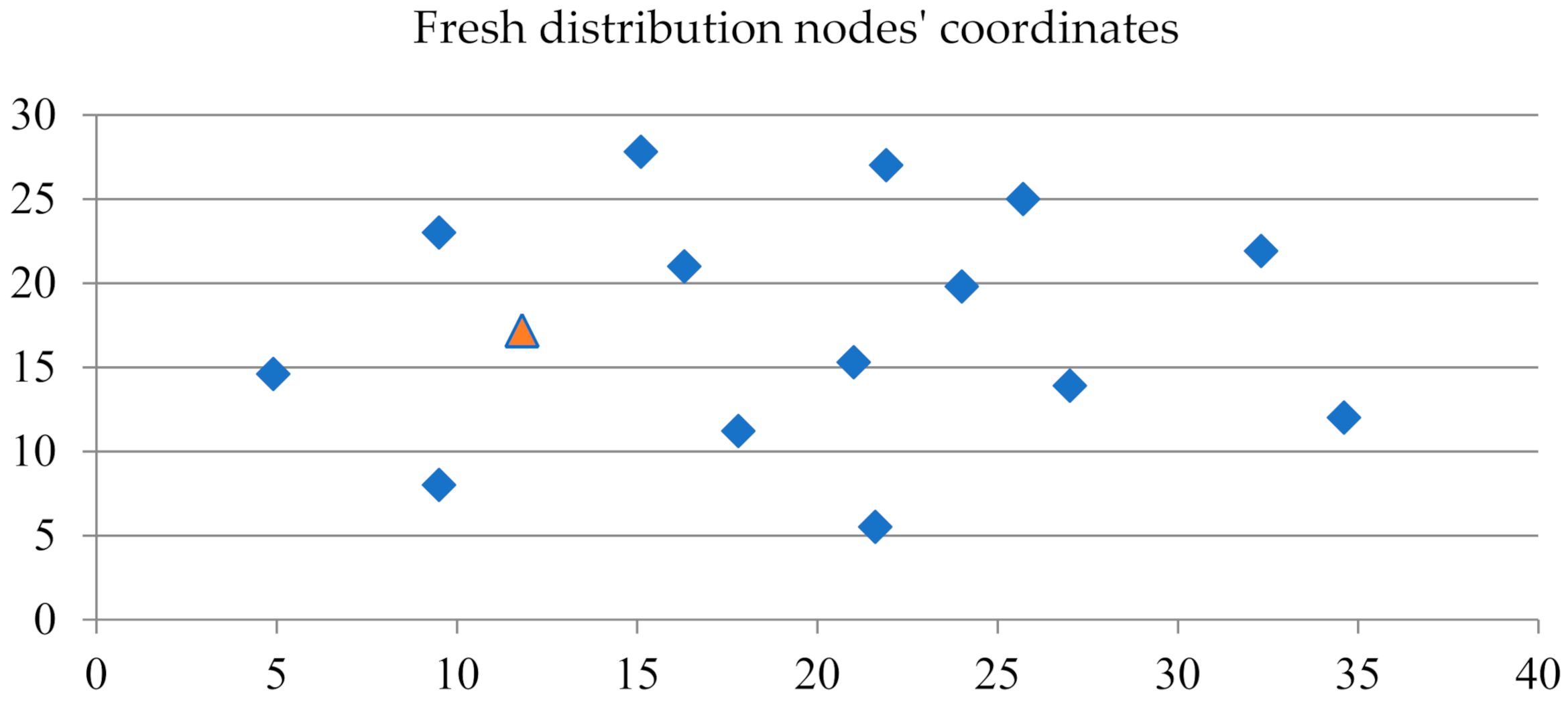
Table 1 shows the location coordinate data of each demand node.
Figure 3 presents the geographical relationship between the demand node and the delivery center. The triangle indicates the location of the distribution center. The topology of the network is fixed in this situation.
The triangle in
Figure 3 represents the point ‘A’, which is a distribution center, and other rhombuses represent demand nodes. Based on the formulation of the problem in
Section 3, the demand of each node is expected to follow certain random distributions. Each demand node has its own time window.
Table 2 presents a summary of the expected demand and the time window of each demand node.
With the assumption made in the formulation of the problem in
Section 3, the value of the main parameter in the formulation is estimated based on the real distribution tasks in a specific situation.
Table 3 presents a summary of the estimation of main parameters in the example.
By collecting and analyzing a large amount of actual data with respect to the road capacity and the importance of each route, the unblocked reliability between nodes is calculated according to Equation (3).
Table 4 presents a summary of the unblocked reliability between demand nodes in the problem.
There is an uncertain demand in each demand node for fresh products in this situation. The demand of each node is subject to an independent normal distribution X~N (μ, σ2), and , σ is the standard deviation. It measures the dispersion degree of the customer demand. This is used to approximate the uncertainty of the customer demand in a given situation.
The data parameters are input into MATLAB with respect to Algorithm 1 as above for determining the optimal delivery route with the demand satisfaction rate at 95%. In searching for the optimal delivery route, 50 tests are conducted for each random condition. To test the effectiveness of the improved algorithm under different degrees of dispersion, different standard deviations
σ to 1, 2, 3, 4, 5 and 6 are tested.
Table 5 shows the results.
As shown in
Table 5, the path optimization results can be obtained under different values of
σ. For example, when
σ = 2, the optimal delivery route of this uncertain model is as follows:
,
,
.
Table 5 shows that the improved algorithm performs better under the condition of involving different dispersion degrees.
Figure 4 presents an overall trend of the optimization process under different values of
σ.
Figure 5 presents a comparative analysis result. The improved algorithm shows certain advantages in terms of the convergence speed and the ability of searching for the optimal solution. Compared with the original algorithm, the improved algorithm has fewer iterations when it converges. This indicates that the convergence speed of the improved algorithm is faster, and the individual solutions are not stuck in a local optimal. Furthermore, the accuracy of the optimal solution is increased, and the distribution cost is reduced with the use of the improved algorithm.
Further analysis has been conducted on exploring the relationship between the total distribution costs and the volatility of the uncertain customer demand through changing the value of σ in the experiment. The result shows that the total distribution cost increases when the customer demand is volatile. The distribution of fresh products has special requirements in terms of logistics’ time, temperature and tolerance. The volatility of the uncertain demand directly affects the cargo damage cost and the shortage cost. This means that fresh product distribution companies should better understand the customer demand to reduce the impact of uncertainty fluctuations on the delivery cost. Furthermore, it is critical to maintain the relationship between business and customers for the overall cost reduction.


