
Fear in a Handful of Dust: The Epidemiological, Environmental, and Economic Drivers of Death by PM2.5 Pollution


Abstract
1. Introduction
1.1. PM2.5 Air Pollution
1.2. The Environmental Kuznets Curve
- (a)
- An inverted U-shaped relationship represents the canonical environmental Kuznets curve. The inverted U describes environmental degradation in three stages. At first, increasing pollution from accelerated exploitation of natural resources shows a scale effect. A composition effect then takes over, emphasizing cleaner activities in production. During this intermediate stage, the pollution rate stagnates despite economic growth. A final techniques effect takes hold as increased economic development replaces obsolete technologies with cleaner ones and reduces pollution [56,57,58,59]. An alternative account for the emergence of the inverted U-shaped curve attributes superior environmental performance at higher income levels to environmental transition theory, by which better developed economies export pollution-intensive activities to less developed trade partners [60,61,62].
- (b)
- (c)
- An N-shaped relationship combines the dynamics of the inverted U and the monotonic increase. At lower levels of development, the inverted U describes the relationship between economic productivity and environmental degradation. Beyond a certain income level, however, development exerts monotonically increasing pressure on the environment [63] (p. 865); [65,66,67].
1.3. An Overview of This Article
2. Materials and Methods
2.1. Data
2.1.1. Dependent and Independent Variables
- expectancy—Life expectancy at birth (in years)
- poverty_threshold—The threshold at which a single person is at risk of poverty (in euros)
- poverty_excluded—The rate of risk from poverty before social transfers (with pensions excluded from the definition of social transfers)
- poverty_included—The rate of risk from poverty before social transfers (with pensions included in the definition of social transfers)
- emissions—PM2.5 emissions (in kilograms per capita)
- exposure—Mean annual exposure to PM2.5 pollution (in µg/m3)
- Five morbidity indicators—The incidence in persons older than 65 years of the following diseases:
- cardio_incidence—cardiovascular disease
- ischemic_incidence—ischemic heart disease
- copd_incidence—chronic obstructive pulmonary disease (COPD)
- asthma_incidence—asthma
- tracheal_incidence—tracheal, bronchial, and lung cancer (hereinafter designated as “tracheal cancer” as shorthand covering all three types of cancer)
- Five mortality indicators designated as cardio_death, ischemic_death, copd_death, asthma_death, and tracheal_incidence: The rate of premature death among persons older than 65 from each of the preceding five diseases
- real_gdp_pc—Real gross domestic product (GDP) per capita
- health_expenditures—Health-related government expenditures per capita
- environmental_taxes—Environmentally related taxes as a percentage of GDP
- social_contributions—Social security contributions as a percentage of GDP
- spending—Overall government spending per capita
- corruption—Corruption perception index
- gini—The Gini coefficient of economic inequality
2.1.2. Endogeneity and the IVS2LS Model
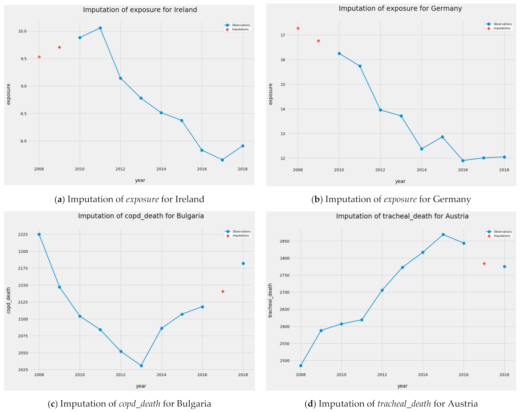
2.1.3. The Imputation of Missing Values
2.2. Data Preprocessing and Other Preparatory Details
2.2.1. Splitting and Scaling
2.2.2. Beta Coefficients
2.2.3. The Bias-Variance Tradeoff and Hyperparameter Tuning
2.3. Predictive and Supervised Methods
2.3.1. Conventional Linear Models
2.3.2. Supervised Machine Learning
- Linear models:
- ○
- Pooled OLS
- ○
- Fixed entity effects (FEE)
- ○
- Fixed time effects (FTE)
- ○
- Fixed entity and time effects (FETE)
- ○
- Random effects (RE)
- ○
- Instrumental variable/two-stage least squares (IV2SLS)
- Machine learning models
- ○
- Conventional decision tree ensembles
- ▪
- Random forests
- ▪
- Extra trees
- ○
- AdaBoost
- ○
- Gradient boosting models:
- ▪
- Gradient boosting in SciKit-Learn
- ▪
- XGBoost
- ▪
- LightGBM
2.3.3. Interpreting and Synthesizing Machine Learning through Feature Importances
2.3.4. Stacking Generalization
2.4. Unupervised Methods
2.4.1. Unsupervised Machine Learning in Overview
2.4.2. Clustering through Affinity Propagation
2.4.3. Dimensionality Reduction through Manifold Learning
2.4.4. Novel Contributions to Unsupervised Machine Learning
3. Results
3.1. Linear Models
3.1.1. Parameters and Statistical Significance
3.1.2. Fitted Values and Model Accuracy
3.2. Supervised Machine Learning Models
3.2.1. Fitted Values and Model Accuracy
3.2.2. Feature Importances
3.3. Emulated Feature Importances of Linear Models
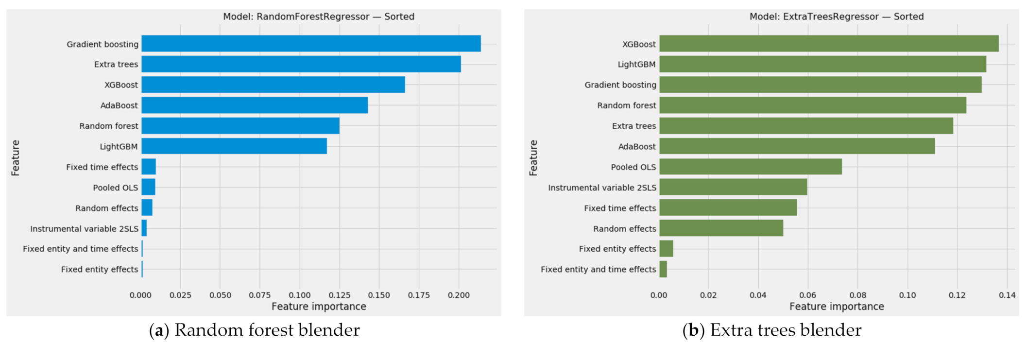
3.4. Stacking Generalization
3.4.1. Aggregated Predictions
3.4.2. The Combined Array of Feature Importances
3.4.3. Aggregated Feature Importances
3.5. Unsupervised Machine Learning on Country-Level Aggregate Data
- Cluster 0; Austria, Belgium, Finland, France, Germany, Greece, Italy, Luxembourg, Malta, the Netherlands, Sweden
- Cluster 1: Croatia, Hungary, Poland, Slovenia
- Cluster 2: Czechia, Slovakia
- Cluster 3: Denmark
- Cluster 4: Bulgaria, Estonia, Latvia, Lithuania, Romania
- Cluster 5: Cyprus, Ireland, Portugal, Spain
- Cluster 0: Bulgaria
- Cluster 1: Austria, Belgium, France, Germany, Lithuania, Malta, and the Netherlands
- Cluster 2: Croatia, Czechia, Hungary, Latvia, Romania, and Slovakia
- Cluster 3: Denmark, Estonia, Finland, Ireland, Luxembourg, Portugal, Spain, and Sweden
- Cluster 4: Poland
- Cluster 5: Cyprus, Greece, Italy, and Slovenia
3.6. Unsupervised Machine Learning on the Entire PM2.5 Dataset
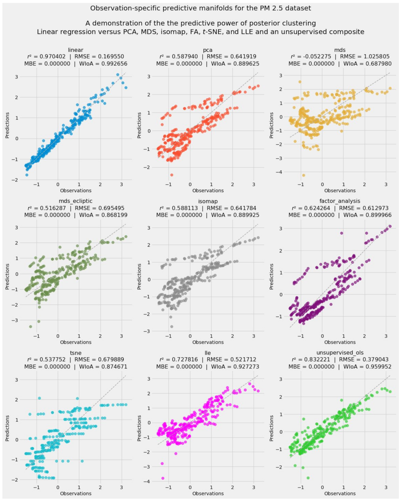
3.6.1. The Accuracy-Weighted Array Reveals Visually Linear Convergence in the Data
3.6.2. Predictive Unsupervised Learning
- Principal component analysis (PCA)
- Multidimensional scaling (MDS)
- Isometric feature mapping (isomap)
- Factor analysis
- t-distributed stochastic neighbor embedding (t-SNE)
- Locally linear embedding (LLE)
- Actual feature importances from supervised machine learning models
- Emulated feature importances from linear models such as pooled OLS and all variants of fixed effects
- The weighting of actual and emulated feature importances according to the model-specific feature importances generated by the stacking blender
3.7. The Environmental Kuznets Curve
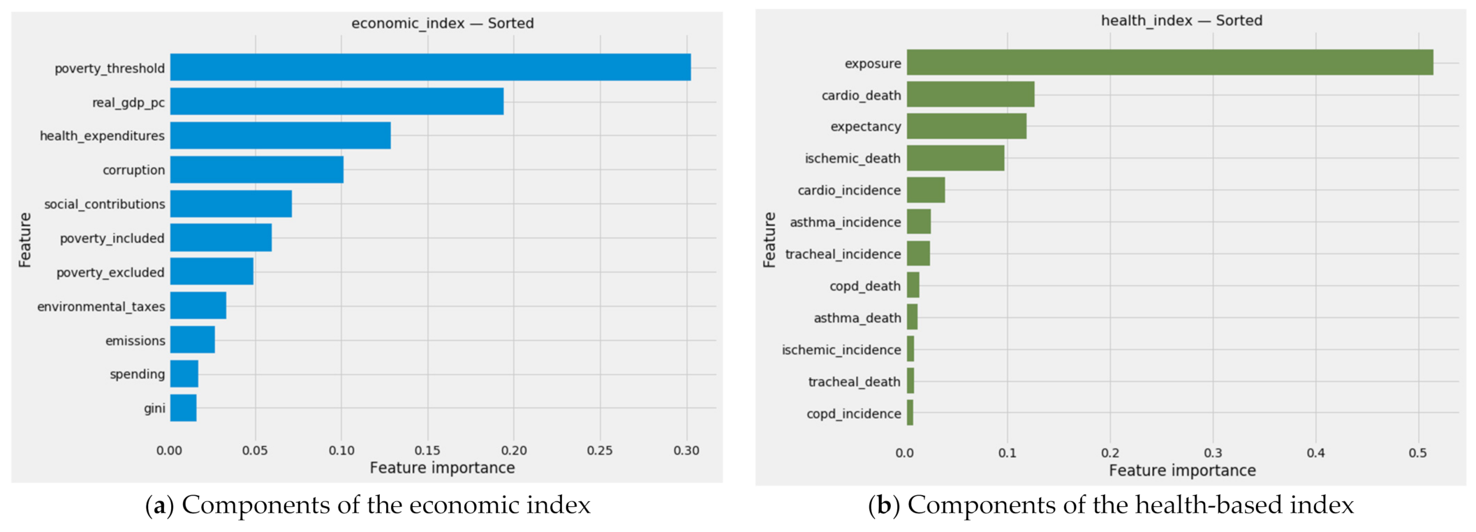
3.7.1. Extracting Economic and Health-Based Indexes through PCA
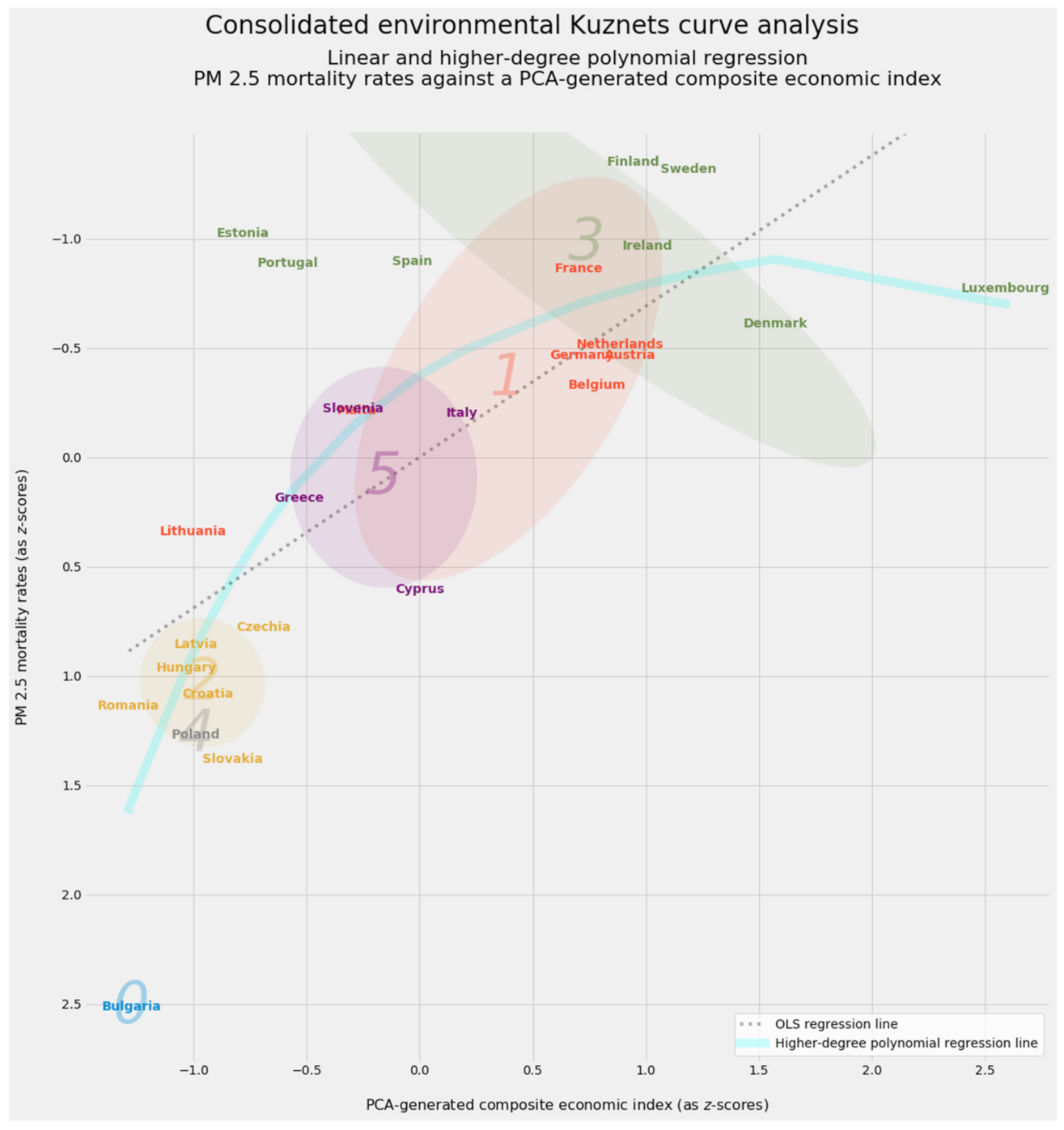
3.7.2. The Economic Variant of the Environmental Kuznets Curve
- The healthy countries in clusters 3 and most of cluster 1
- An intermediate tier consisting of cluster 5 and two countries in cluster 1
- Clusters 2, 4, and 0, including impoverished and unhealthy Bulgaria on its own
3.7.3. A Health-Based Look at the Environmental Kuznets Curve
4. Discussion
4.1. The Environmental Kuznets Curve: Bridging Quantitative Analysis with Policy Evaluation
4.1.1. An Apt Metaphor for Unsupervised Machine Learning Writ Large
4.1.2. Closer Examination of Health-Based Factors
4.2. Cluster- and Country-Specific Analysis of Individual EU-27 Member States
4.3. Policymaking at the European Level: Implications and Recommendations
5. Conclusions
- Conventional linear models
- ○
- Pooled OLS
- ○
- Fixed effect models
- ○
- Random effects
- ○
- Instrumental value, two-stage least squares
- Supervised machine learning alternatives to linear regression
- ○
- Decision tree ensembles such as random forests and extra trees
- ○
- Boosting models such as AdaBoost, XGBoost, and LightGBM
- Stacking generalization
- ○
- As an aggregator of predictions
- ○
- As an aggregator of real and emulated feature importances to advance interpretation and causal inference
- Unsupervised machine learning
- ○
- Clustering
- ○
- Manifold learning
- ○
- A suite of unsupervised methods leading to predictive manifolds
- Environmental Kuznets curves
Author Contributions
Funding
Institutional Review Board Statement
Informed Consent Statement
Data Availability Statement
Acknowledgments
Conflicts of Interest
Appendix A
- 0.
- Premature death rates attributable to PM2.5 pollution: This data appears in the OECD repository, “Mortality, Morbidity and Welfare Cost from Exposure to Environment-Related Risks.” Data for 2018 is derived from “Premature death rates attributable to outdoor air pollution (PM2.5); Crude death rate per 100,000 population.” Data for 2008 through 2017 is derived from “Premature deaths from ambient particulate matter for persons more than 64 years old, both sexes.”
- 1.
- Life expectancy at birth (in years) is the average number of years a newborn is expected to live if mortality patterns at the time of its birth remain constant in the future. It reflects the overall mortality level of a population, and summarizes the mortality pattern that prevails across all age groups in a given year. It is calculated in a period life table that provides a snapshot of a population’s mortality pattern at a given time.
- 2.
- The threshold at which a single person is at risk of poverty (in euros) is determined by calculating the equivalized income per household member for all households. Afterwards, the middle value (the median) of the income distribution is determined and 60 percent of the median is determined as the risk-of-poverty threshold. Everyone with the income below the threshold is in a worse situation than others, but they do not necessarily live in deprivation. The at-risk-of-poverty threshold is presented in currencies, while the at-risk-of-poverty rate is presented in relative terms as a percentage.
- 3.
- The rate of risk from poverty before social transfers (with pensions excluded from the definition of social transfers) is calculated as the percentage of people (or thousands of people) who are at risk of poverty, based on the equivalized disposable income before all social transfers—excluding pensions, over the total population.
- 4.
- The rate of risk from poverty before social transfers (with pensions included in the definition of social transfers) is calculated as the percentage of people (or thousands of people) who are at-risk-of-poverty, based on the equivalized disposable income before all social transfers—including pensions, over the total population.
- 5.
- PM2.5 emissions (in kilograms per capita) show population-weighted emissions of PM2.5. Fine particulates (PM2.5) are those whose diameters are less than 2.5 micrometers. Particulates can be carried deep into the lungs where they can cause inflammation and a worsening of the condition of people with heart and lung diseases. The smaller the particles, the deeper they travel into the lungs, with more potential for harm. Air emissions accounts record the flows of residual gaseous and particulate materials emitted by resident units and flowing into the atmosphere. Air emissions accounts record emissions arising from all resident units (=economic activities), regardless of where these emissions actually occur geographically. A unit is said to be a resident unit of a country when it has a center of economic interest in the economic territory of that country, that is, when it engages for an extended period (1 year or more) in economic activities in that territory.
- 6.
- Mean annual exposure to PM2.5 pollution (in µg/m3) reflects the estimated annual mean exposure level of an average resident to outdoor particulate matter, expressed as population-weighted PM2.5 levels. The underlying PM2.5 estimates are taken from the Global Burden of Disease (GBD) 2019 project. They are derived by integrating satellite observations, chemical transport models, and measurements from ground monitoring station networks.
- 7.
- Five morbidity indicators: The incidence in persons older than 65 years of the following diseases: a. cardiovascular disease: any disease of the circulatory system, namely the heart (cardio) or blood vessels (vascular). Includes ACS, angina, stroke, and peripheral vascular disease. Also known as circulatory disease. b. ischemic heart disease: also heart attack and angina (chest pain). Also known as coronary heart disease. c. chronic obstructive pulmonary disease (COPD): chronic respiratory diseases (CRDs) are diseases of the airways and other structures of the lung. d. asthma: it is a disease characterized by recurrent attacks of breathlessness and wheezing, which vary in severity and frequency from person to person. This condition is due to inflammation of the air passages in the lungs and affects the sensitivity of the nerve endings in the airways so they become easily irritated. In an attack, the lining of the passages swell causing the airways to narrow and reducing the flow of air in and out of the lungs. e. tracheal, bronchial, and lung cancer (hereinafter designated as “tracheal cancer” as shorthand covering all three types of cancer): tracheal cancer is cancer that forms in tissue of the airway that leads from the larynx (voice box) to the bronchi (large airways that lead to the lungs). Tracheal is also called windpipe. Bronchus cancer is cancer that begins in the tissue that lines or covers the airways of the lungs, including small cell and non-small cell lung cancer. Lung cancer is cancer that forms in tissues of the lung, usually in the cells lining air passages. The two main types are small cell lung cancer and non-small cell lung cancer. These types are diagnosed based on how the cells look under a microscope.
- 8.
- Five mortality indicators: The rate of premature death among persons older than 65 years from each of the preceding five diseases: number of people with incidence of cardiovascular diseases, ischemic heart disease, chronic obstructive pulmonary disease (COPD), asthma, and tracheal, bronchus, and lung cancer; ages above 65, according to the GBD study.
- 9.
- Real gross domestic product (GDP) per capita is calculated as the ratio of real GDP to the average population of a specific year. GDP measures the value of total final output of goods and services produced by an economy within a certain period of time. It includes goods and services that have markets (or which could have markets) and products which are produced by general government and non-profit institutions.
- 10.
- Health-related government expenditures per capita tracks all health spending in a given country over a defined period of time regardless of the entity or institution that financed and managed that spending. It generates consistent and comprehensive data on health spending in a country, which in turn can contribute to evidence-based policymaking.
- 11.
- Environmentally related taxes as a percentage of GDP are important instrument for governments to shape relative prices of goods and services. The characteristics of such taxes included in the database (e.g., revenue, tax base, tax rates, exemptions, etc.) are used to construct the environmentally related tax revenues with a breakdown by environmental domain: energy products (including vehicle fuels); motor vehicles and transport services; measured or estimated emissions to air and water, ozone depleting substances, certain non-point sources of water pollution, waste management and noise, as well as management of water, land, soil, forests, biodiversity, wildlife, and fish stocks.
- 12.
- Social security contributions as a percentage of GDP are paid on a compulsory or voluntary basis by employers, employees and self- and non-employed persons, shown as a percentage of GDP.
- 13.
- Overall government spending per capita captures the burden imposed by government expenditures, which includes consumption by the state and all transfer payments related to various entitlement programs.
- 14.
- The corruption perception index scores and ranks countries/territories based on how corrupt a country’s public sector is perceived to be by experts and business executives. It is a composite index, a combination of 13 surveys and assessments of corruption, collected by a variety of reputable institutions. Corruption generally comprises illegal activities, which are deliberately hidden and only come to light through scandals, investigations, or prosecutions.
- 15.
- The Gini coefficient of economic inequality is defined as the relationship of cumulative shares of the population arrange according to the level of equivalized disposable income, to the cumulative share of the equivalized total disposable income received by them.
- 16.
- The welfare cost of premature deaths per capita among elderly persons from PM2.5 and PM10 combined shows the welfare cost of premature deaths per capita among elderly persons from PM2.5 and PM10. Fine and coarse particulates (PM10) are those whose diameter is less than 10 micrometers, while fine particulates (PM2.5) are those whose diameters are less than 2.5 micrometers. Particulates can be carried deep into the lungs where they can cause inflammation and a worsening of the condition of people with heart and lung diseases.
- 17.
- The welfare cost of premature deaths per capita among elderly persons from PM2.5 alone shows data on mortality from exposure to environmental risks are taken from GBD (2019), Global Burden of Disease Study 2019 Results. Welfare costs are calculated using a methodology adapted from OECD (2017b), The Rising Cost of Ambient Air Pollution thus far in the 21st Century: Results from the BRIICS and the OECD Countries.
Appendix B


References
- WHO. Social and gender inequalities in environment and health. In Proceedings of the Fifth Ministerial Conference on Environment and Health. Protecting Children’s Health in a Changing Environment, Parma, Italy, 10–12 March 2010; Publications WHO Regional Office for Europe: Copenhagen, Denmark, 2010. [Google Scholar]
- Kelly, F.J.; Fussell, J.C. Air pollution and public health: Emerging hazards and improved understanding of risk. Environ. Geochem. Health 2015, 37, 631–649. [Google Scholar] [CrossRef] [PubMed]
- WHO Regional Office for Europe, OECD. Economic Cost of the Health Impact of Air Pollution in Europe: Clean Air, Health and Wealth; WHO Regional Office for Europe: Copenhagen, Denmark, 2015. [Google Scholar]
- Pope, C.A., III; Dockery, D.W. Health effects of fine particulate air pollution: Lines that connect. J. Air Waste Manag. Assoc. 2006, 56, 709–742. [Google Scholar] [CrossRef] [PubMed]
- EEA. Particulate Matter from Natural Sources and Related Reporting under the EU Air Quality Directive in 2008 and 2009; EEA Technical Report No 10/2012; Publications Office of the European Union: Luxembourg, 2012. [Google Scholar] [CrossRef]
- EEA. Air Quality in Europe—2020 Report; EEA Report No 09/2020; Publications Office of the European Union: Luxembourg, 2020. [Google Scholar] [CrossRef]
- Wilson, W.E.; Suh, H.H. Fine particles and coarse particles: Concentration relationships relevant to epidemiologic studies. J. Air Waste Manag. Assoc. 1997, 47, 1238–1249. [Google Scholar] [CrossRef]
- UNECE. Convention on Long-range Transboundary Air Pollution. 1979. Available online: https://unece.org/fileadmin/DAM/env/lrtap/full%20text/1979.CLRTAP.e.pdf (accessed on 19 July 2021).
- WHO. Air Quality Guidelines for Particulate Matter, Ozone, Nitrogen Dioxide and Sulfur Dioxide: Global Update 2005, Summary of Risk Assessment. (WHO/SDE/PHE/OEH/06.02). Available online: https://apps.who.int/iris/bitstream/handle/10665/69477/WHO_SDE_PHE_OEH_06.02_eng.pdf;jsessionid=C9C44FEBF1206620771CDD21AA56EBCE?sequence=1 (accessed on 19 July 2021).
- Directive 2008/50/EC of the European Parliament and of the Council of 21 May 2008 on ambient air quality and cleaner air for Europe. Off. J. Eur. Union. Available online: https://eurlex.europa.eu/legalcontent/en/ALL/?uri=CELEX%3A32008L0050 (accessed on 19 July 2021).
- EEA. Air Quality in Europe—2018 Report. EEA Report No 12/2018. 2018. Available online: https://www.eea.europa.eu/publications/air-quality-in-europe-2018 (accessed on 19 July 2021).
- IARC. Outdoor Air Pollution a Leading Environmental Cause of Cancer Deaths. 2013. Available online: https://www.iarc.who.int/wp-content/uploads/2018/07/pr221_E.pdf (accessed on 19 July 2021).
- Cohen, A.J.; Ross Anderson, H.; Ostro, B.; Pandey, K.D.; Krzyzanowski, M.; Künzli, N.; Gutschmidt, K.; Pope, A.; Romieu, I.; Samet, J.M.; et al. The global burden of disease due to outdoor air pollution. J. Toxicol. Environ. Health A 2005, 68, 1301–1307. [Google Scholar] [CrossRef] [PubMed]
- Lelieveld, J.; Evans, J.S.; Fnais, M.; Giannadaki, D.; Pozzer, A. The contribution of outdoor air pollution sources to premature mortality on a global scale. Nature 2015, 525, 367–371. [Google Scholar] [CrossRef] [PubMed]
- Matkovic, V.; Mulić, M.; Azabagić, S.; Jevtić, M. Premature adult mortality and years of life lost attributed to long-term exposure to ambient particulate matter pollution and potential for mitigating adverse health effects in Tuzla and Lukavac, Bosnia and Herzegovina. Atmosphere 2020, 11, 1107. [Google Scholar] [CrossRef]
- Stanaway, J.D.; Afshin, A.; Gakidou, E.; Lim, S.S.; Abate, D.; Abate, K.H.; Abbafati, C.; Abbasi, N.; Abbastabar, H.; Abd-Allah, F.; et al. Global, regional, and national comparative risk assessment of 84 behavioural, environmental and occupational, and metabolic risks or clusters of risks for 195 countries and territories, 1990–2017: A systematic analysis for the Global Burden of Disease Study 2017. Lancet 2018, 392, 1923–1994. [Google Scholar] [CrossRef]
- Correia, A.W.; Pope, C.A., III; Dockery, D.W.; Wang, Y.; Ezzati, M.; Dominici, F. The effect of air pollution control on life expectancy in the United States: An analysis of 545 US counties for the period 2000 to 2007. Epidemiology 2013, 24, 23–31. [Google Scholar] [CrossRef]
- EEA. Healthy Environment, Healthy Lives: How the Environment Influences Health and Well-Being in Europe; Publications Office of the European Union: Luxembourg, 2019. [Google Scholar]
- Pope, C.A.; Muhlestein, J.B.; May, H.T.; Renlund, D.G.; Anderson, J.L.; Horne, B.D. Ischemic heart disease events triggered by short-term exposure to fine particulate air pollution. Circulation 2006, 114, 2443–2448. [Google Scholar] [CrossRef]
- Wong, C.M.; Tsang, H.; Lai, H.K.; Thomas, G.N.; Lam, K.B.; Chan, K.P.; Zheng, Q.; Ayres, J.G.; Lee, S.Y.; Lam, T.H.; et al. Cancer mortality risks from long-term exposure to ambient fine particle. Cancer Epidemiol. Biomark. Prev. 2016, 25, 839–845. [Google Scholar] [CrossRef]
- Al-Hemoud, A.; Gasana, J.; Al-Dabbous, A.; Al-Shatti, A.; Al-Khayat, A. Disability adjusted life years (DALYs) in terms of years of life lost (YLL) due to premature adult mortalities and postneonatal infant mortalities attributed to PM2.5 and PM10 exposures in Kuwait. Int. J. Environ. Res. Pub. Health 2018, 15, 2609. [Google Scholar] [CrossRef]
- Maciejewska, K. Short-term impact of PM2.5, PM10, and PMc on mortality and morbidity in the agglomeration of Warsaw, Poland. Air Qual. Atmos. Health 2020, 13, 659–672. [Google Scholar] [CrossRef]
- Hayes, R.B.; Lim, C.; Zhang, Y.; Cromar, K.; Shao, Y.; Reynolds, H.R.; Silverman, D.T.; Jones, R.R.; Park, Y.; Jerrett, M.; et al. PM2.5 air pollution and cause-specific cardiovascular disease mortality. Int. J. Epidemiol. 2019, 49, 25–35. [Google Scholar] [CrossRef] [PubMed]
- Dominici, F.; Peng, R.D.; Bell, M.L.; Pham, L.; McDermott, A.; Zeger, S.L.; Samet, J.M. Fine particulate air pollution and hospital admission for cardiovascular and respiratory diseases. J. Am. Med. Assoc. 2006, 295, 1127–1134. [Google Scholar] [CrossRef] [PubMed]
- Cao, Q.; Rui, G.; Liang, Y. Study on PM2.5 pollution and the mortality due to lung cancer in China based on geographic weighted regression model. BMC Pub. Health 2018, 18, 925. [Google Scholar] [CrossRef]
- Turner, M.C.; Andersen, Z.J.; Baccarelli, A.; Diver, W.R.; Gapstur, S.M.; Pope, C.A.; Prada, D.; Samet, J.; Thurston, G.; Cohen, A. Outdoor air pollution and cancer: An overview of the current evidence and public health recommendations. CA: Cancer J. Clin. 2020, 70, 460–479. [Google Scholar] [CrossRef]
- Simoni, M.; Baldacci, S.; Maio, S.; Cerrai, S.; Sarno, G.; Viegi, G. Adverse effects of outdoor pollution in the elderly. J. Thorac. Dis. 2015, 7, 34–45. [Google Scholar] [CrossRef] [PubMed]
- Jung, E.-J.; Na, W.; Lee, K.-E.; Jang, J.-Y. Elderly mortality and exposure to fine particulate matter and ozone. J. Korean Med. Sci. 2019, 34, e311. [Google Scholar] [CrossRef] [PubMed]
- Eurostat. Population Structure and Ageing, Statistics Explained. 2020. Available online: https://ec.europa.eu/eurostat/statisticsexplained/index.php/Population_structure_and_ageing (accessed on 19 July 2021).
- OECD/EU. Health at a Glance: Europe 2018: State of Health in the EU Cycle; OECD Publishing: Paris, France, 2018. [Google Scholar] [CrossRef]
- Staatsen, B.; van der Vliet, N.; Kruize, H.; Hall, L.; Guillen-Hanson, G.; Modee, K.; Strube, R.; Lippevelde, W.; Buytaert, B. Inherit: Exploring Triple-Win Solutions for Living, Moving and Consuming that Encourage Behavioural Change, Protect the Environment, Promote Health and Health Equity; EuroHealthNet: Brussels, Belgium, 2017. Available online: https://www.semanticscholar.org/paper/Exploring-triple-win-solutions-for-living%2C-moving-Staatsen-Vliet/9d8a8c6e20dc3b3d98969ff507f9b8b65c4d33c1 (accessed on 19 July 2021).
- United Nations, Department of Economic and Social Affairs, Population Division. World Population Ageing 2019: Highlights (ST/ESA/SER.A/430). 2019. Available online: https://www.un.org/en/development/desa/population/publications/pdf/ageing/WorldPopulationAgeing2019-Report.pdf (accessed on 19 July 2021).
- Miranda, M.L.; Edwards, S.E.; Keating, M.H.; Paul, C.J. Making the environmental justice grade: The relative burden of air pollution exposure in the United States. Int. J. Environ. Res. Pub. Health 2011, 8, 1755–1771. [Google Scholar] [CrossRef]
- Bell, M.L.; Ebisu, K. Environmental inequality in exposures to airborne particulate matter components in the United States. Environ. Health Perspect. 2012, 120, 1599–1704. [Google Scholar] [CrossRef]
- WHO and Europe. Social Inequalities and Their Influence on Housing Risk Factors and Health; World Health Organization Regional Office for Europe: Copenhagen, Denmark, 2009; Available online: http://www.euro.who.int/__data/assets/pdf_file/0013/113260/E92729.pdf (accessed on 19 July 2021).
- Janssen, N.A.; Gerlofs-Nijland, M.E.; Lanki, T.; Salonen, R.O.; Cassee, F.; Hoek, G.; Fischer, P.; Brunekreef, B.; Krzyzanowski, M. Health Effects of Black Carbon; World Health Organization: Copenhagen, Denmark, 2012. [Google Scholar]
- Li, Y.; Henze, D.K.; Jack, D.; Henderson, B.H.; Kinney, P.L. Assessing public health burden associated with exposure to ambient black carbon in the United States. Sci. Total Environ. 2016, 539, 515–525. [Google Scholar] [CrossRef] [PubMed]
- Aslam, A.; Ibrahim, M.; Shahid, I.; Mahmood, A.; Irshad, M.K.; Yamin, M.; Ghazala, T.M.; Shamshiri, R.R. Pollution characteristics of particulate matter (PM2.5 and PM10) and constituent carbonaceous aerosols in a South Asian future megacity. Appl. Sci. 2020, 10, 8864. [Google Scholar] [CrossRef]
- Bisht, D.S.; Tiwari, S.; Dumka, U.C.; Srivastava, A.K.; Safai, P.D.; Ghude, S.D.; Chate, D.M.; Rao, P.S.; Ali, K.; Prabhakaran, T.; et al. Tethered balloon-born and ground-based measurements of black carbon and particulate profiles within the lower troposphere during the foggy period in Delhi, India. Sci. Total Environ. 2016, 573, 894–905. [Google Scholar] [CrossRef] [PubMed]
- Science for Environment Policy. What are the Health Costs of Environmental Pollution? Future Brief 21. Brief Produced for the European Commission DG Environment by the Science Communication Unit, UWE, Bristol, UK. 2018. Available online: http://ec.europa.eu/science-environment-policy (accessed on 19 July 2021).
- Hunt, A.; Ferguson, J.; Hurley, F.; Searl, A. Social Costs of Morbidity Impacts of Air Pollution; OECD Environment Working Papers, No. 99; OECD Publishing: Paris, France, 2016. [Google Scholar] [CrossRef]
- Lu, J.G. Air pollution: A systematic review of its psychological, economic, and social effects. Curr. Opin. Psychol. 2020, 32, 52–65. [Google Scholar] [CrossRef] [PubMed]
- Bickel, P.; Friedrich, R.; Burgess, A.; Fagiani, P.; Hunt, A.; de Jong, G.; Laird, J.; Lieb, C.; Lindberg, G.; Mackie, P. Developing Harmonised European Approaches for Transport Costing and Project Assessment (HEATCO). Proposal for Harmonised Guidelines. Deliverable 5; Universität Stuttgart: Stuttgart, Germany, 2006. Available online: http://heatco.ier.unistuttgart.de/HEATCO_D5.pdf (accessed on 19 July 2021).
- Dechezleprêtre, A.; Rivers, N.; Stadler, B. The Economic Cost of Air Pollution: Evidence from Europe; OECD Economics Department Working Papers, No. 1584; OECD Publishing: Paris, France, 2019. [Google Scholar] [CrossRef]
- Grossman, G.M.; Krueger, A.B. Environmental impacts of the North American Free Trade Agreement. In The Mexico-U.S. Free Trade Agreement; Garber, P.M., Ed.; MIT Press: Cambridge, MA, USA, 1994; pp. 13–56. [Google Scholar]
- Grossman, G.M.; Krueger, A.B. Economic growth and the environment. Q. J. Econ. 1995, 110, 353–377. [Google Scholar] [CrossRef]
- Bo, S. A literature survey on environmental Kuznets curve. Energy Procedia 2011, 5, 1322–1325. [Google Scholar] [CrossRef]
- Dasgupta, S.; Laplante, B.; Wang, H.; Wheeler, D. Confronting the environmental Kuznets curve. J. Econ. Perspect. 2002, 16, 147–168. [Google Scholar] [CrossRef]
- Dinda, S. Environmental Kuznets curve hypothesis: A survey. Ecol. Econ. 2004, 49, 431–455. [Google Scholar] [CrossRef]
- Goldman, B. Meta-Analysis of Environmental Kuznets Curve Studies: Determining the Cause of the Curve’s Presence. Park Place Econ. 2012, 20, 10. Available online: https://digitalcommons.iwu.edu/parkplace/vol20/iss1/10 (accessed on 19 July 2021).
- Maneejuk, N.; Ratchakom, S.; Maneejuk, P.; Yamaka, W. Does the environmental Kuznets curve exist? An international study. Sustainability 2020, 12, 9117. [Google Scholar] [CrossRef]
- Stern, D.I. The rise and fall of the environmental Kuznets curve. World Dev. 2004, 32, 1419–1439. [Google Scholar] [CrossRef]
- Kuznets, S. Economic growth and income inequality. Am. Econ. Rev. 1955, 45, 1–28. [Google Scholar]
- Lieb, C.M. The environmental Kuznets curve and flow versus stock pollution: The neglect of future damages. Environ. Resour. Econ. 2004, 29, 483–506. [Google Scholar] [CrossRef]
- Mosconi, E.M.; Colantoni, A.; Gambella, F.; Cudlinová, E.; Salvati, L.; Rodrigo-Comino, J. Revisiting the environmental Kuznets curve: The spatial interaction between economy and territory. Economies 2020, 8, 74. [Google Scholar] [CrossRef]
- Abrate, G.; Ferraris, M. The Environmental Kuznets Curve in the Municipal Solid Waste Sector. HERMES: Higher Education Research on Mobility Regulation and the Economics of Local Services, Working Paper No. 1. 2010. Available online: https://citeseerx.ist.psu.edu/viewdoc/download?doi=10.1.1.637.2954&rep=rep1&type=pdf (accessed on 19 July 2021).
- Chen, Y.; Lee, C.C.; Chen, M. Ecological footprint, human capital, and urbanization. Energy Environ. 2021, in press. [Google Scholar] [CrossRef]
- Ekins, P. The Kuznets curve for the environment and economic growth: Examining the evidence. Environ. Plan A 1997, 29, 805–830. [Google Scholar] [CrossRef]
- Kılıç, C.; Balan, F. Is there an environmental Kuznets inverted-U shaped curve? Panoeconomicus 2018, 65, 79–94. [Google Scholar] [CrossRef]
- Majeed, M.T.; Mazhar, M. Reexamination of environmental Kuznets curve for ecological footprint: The role of biocapacity, human capital, and trade. Pak. J. Commer. Soc. Sci. 2020, 14, 202–254. [Google Scholar] [CrossRef]
- Muhammad, S.; Long, X.; Salman, M.; Dauda, L. Effect of urbanization and international trade on CO2 emissions across 65 belt and road initiative countries. Energy 2020, 196, 117102. [Google Scholar] [CrossRef]
- Zaeid, Y.B.; Cheikh, N.B.; Nguyen, P. Long-run analysis of environmental Kuznets curve in the Middle East and north Africa. Environ. Econ. 2017, 8, 72–79. [Google Scholar] [CrossRef]
- Akbostancı, E.; Türüt-Aşık, S.; Tunç, G.İ. The relationship between income and environment in Turkey: Is there an environmental Kuznets curve? Energy Policy 2009, 37, 861–867. [Google Scholar] [CrossRef]
- Bagliani, M.; Bravo, G.; Dalmazzone, S. A consumption-based approach to environmental Kuznets curves using the ecological footprint indicator. Ecol. Econ. 2008, 65, 650–661. [Google Scholar] [CrossRef]
- Allard, A.; Tasman, J.; Uddin, G.S.; Ahmed, A. The N-shaped environmental Kuznets curve: An empirical evaluation using a panel quantile regression approach. Environ. Sci. Pollut. Res. 2018, 25, 5848–5861. [Google Scholar] [CrossRef] [PubMed]
- De Bruyn, S.M.; Opschoor, J.B. Developments in the throughput-income relationship: Theoretical and empirical observations. Ecol. Econ. 1997, 20, 255–268. [Google Scholar] [CrossRef]
- Steger, T.M.; Egli, H. A dynamic model of the environmental Kuznets curve: Turning point and public policy. In Sustainable Resource Use and Economic Dynamics; Bretschger, L., Smulders, S., Eds.; Springer: Dordrecht, The Netherlands, 2007; pp. 17–34. [Google Scholar]
- Brajer, V.; Mead, R.W.; Xiao, F. Health benefits of tunneling through the Chinese environmental Kuznets curve (EKC). Ecol. Econ. 2008, 66, 674–686. [Google Scholar] [CrossRef]
- Esteve, V.; Tamarit, C. Threshold cointegration and nonlinear adjustment between CO2 and income: The environmental Kuznets curve in Spain, 1857–2007. Energy Econ. 2012, 34, 2148–2156. [Google Scholar] [CrossRef]
- Churchill, S.A.; Inekwe, J.; Ivanovski, K.; Smyth, R. The environmental Kuznets curve in the OECD: 1870–2014. Energy Econ. 2018, 75, 389–399. [Google Scholar] [CrossRef]
- Shahbaz, M.; Solarin, S.A.; Ozturk, I. Environmental Kuznets curve hypothesis and the role of globalization in selected African countries. Ecol. Indic. 2016, 67, 623–626. [Google Scholar] [CrossRef]
- Nuroglu, E.; Kunst, R.M. Kuznets and environmental Kuznets curves for developing countries. In Industrial Policy and Sustainable Growth; Yülek, M., Ed.; Springer: Singapore, 2018; pp. 175–188. [Google Scholar] [CrossRef]
- Armeanu, D.; Vintilă, G.; Andrei, J.V.; Gherghina, Ş.C.; Drăgoi, M.C.; Teodor, C. Exploring the link between environmental pollution and economic growth in EU-28 countries: Is there an environmental Kuznets curve? PLoS ONE 2018, 13, e0195708. [Google Scholar] [CrossRef]
- Mazzanti, M.; Zoboli, R. Municipal waste Kuznets curves: Evidence on socio-economic drivers and policy effectiveness from the EU. Environ. Resour. Econ. 2009, 44, 203. [Google Scholar] [CrossRef]
- Wietzke, F.B. Poverty, inequality, and fertility: The contribution of demographic change to global poverty reduction. Popul. Dev. Rev. 2020, 46, 65–99. [Google Scholar] [CrossRef]
- Fang, Z.; Huang, B.; Yang, Z. Trade openness and the environmental Kuznets curve: Evidence from Chinese cities. World Econ. 2020, 43, 2622–2649. [Google Scholar] [CrossRef]
- Gangadharan, L.; Valenzuela, M.R. Interrelationships between income, health and the environment: Extending the environmental Kuznets curve hypothesis. Ecol. Econ. 2001, 36, 513–531. [Google Scholar] [CrossRef]
- Khan, S.A.R.; Zaman, K.; Zhang, Y. The relationship between energy-resource depletion, climate change, health resources and the environmental Kuznets curve: Evidence from the panel of selected developed countries. Renew. Sustain. Energy Rev. 2016, 62, 468–477. [Google Scholar] [CrossRef]
- Costa-Font, J.; Hernandez-Quevedo, C.; Sato, A. A health “Kuznets’ curve”? Cross-sectional and longitudinal evidence on concentration indices. Soc. Indic. Res. 2018, 136, 439–452. [Google Scholar] [CrossRef] [PubMed]
- Fotourehchi, Z.; Çalışkan, Z. Is it possible to describe a Kuznets curve for health outcomes? An empirical investigation. Panoeconomicus 2018, 65, 227–238. [Google Scholar] [CrossRef]
- Zabala, A. Affluence and increased cancer. Nat. Sustain. 2018, 1, 85. [Google Scholar] [CrossRef]
- Talukdar, D.; Seenivasan, S.; Cameron, A.J.; Sacks, G. The association between national income and adult obesity prevalence: Empirical insights into temporal patterns and moderators of the association using 40 years of data across 147 countries. PLoS ONE 2020, 15, e0232236. [Google Scholar] [CrossRef] [PubMed]
- Cleveland, W.S.; Devlin, S.J. Locally weighted regression: An approach to regression analysis by local fitting. J. Am. Stat. Assoc. 1988, 83, 596–610. [Google Scholar] [CrossRef]
- Jacoby, W.G. Loess: A nonparametric, graphical tool for depicting relationships between variables. Elect. Stud. 2000, 19, 577–613. [Google Scholar] [CrossRef]
- De Boor, C. A Practical Guide to Splines; Springer: New York, NY, USA, 1978. [Google Scholar]
- Wegman, E.J.; Wright, I.W. Splines in statistics. J. Am. Stat. Assoc. 1983, 78, 351–365. [Google Scholar] [CrossRef]
- Python. Available online: http://www.python.org (accessed on 19 July 2021).
- Statsmodels. Available online: http://www.statsmodels.org (accessed on 19 July 2021).
- Scipy. Available online: http://www.scipy.org (accessed on 19 July 2021).
- Chen, J.M. An introduction to machine learning for panel data. Int. Adv. Econ. Res. 2021, 27, 1–16. [Google Scholar] [CrossRef]
- Müller, A.C.; Guido, S. Introduction to Machine Learning with Python: A Guide for Data Scientists; O’Reilly Media: Sebastopol, CA, USA, 2017. [Google Scholar]
- Hu, X.; Xie, Z.; Liu, F. Assessment of speckle pattern quality in digital image correlation from the perspective of mean bias error. Measurement 2021, 173, 108618. [Google Scholar] [CrossRef]
- Kato, T. Chapter 4—Prediction of photovoltaic power generation output and network operation. In Integration of Distributed Energy Resources in Power Systems: Implementation, Operation and Control; Funabashi, T., Ed.; Academic Press: London, UK, 2016; pp. 77–100. [Google Scholar] [CrossRef]
- Willmott, C.J. On the validation of models. Phys. Geogr. 1981, 2, 184–194. [Google Scholar] [CrossRef]
- Newman, T.B.; Browner, W.S. In defense of standardized regression coefficients. Epidemiology 1991, 2, 383–386. [Google Scholar] [CrossRef] [PubMed]
- Greenland, S.; Schlesselman, J.J.; Criqui, M.H. The fallacy of employing standardized regression coefficients and correlations as measures of effect. Am. J. Epidemiol. 1986, 123, 203–208. [Google Scholar] [CrossRef]
- Greenland, S.; Maclure, M.; Schlesselman, J.J.; Poole, C.; Morgenstern, H. Standardized regression coefficients: A further critique and review of Some alternatives. Epidemiology 1991, 2, 387–392. [Google Scholar] [CrossRef] [PubMed]
- Criqui, M.H. On the use of standardized regression coefficients. Epidemiology 1991, 2, 393. [Google Scholar] [CrossRef]
- Kohavi, R.; Wolpert, D.H. Bias plus variance decomposition for zero-one loss functions. In Proceedings of the Thirteenth International Conference on Machine Learning, ICML ’96, Bari, Italy, 3–6 July 1996; Morgan Kaufmann Publishers: San Francisco, CA, USA, 1996; pp. 275–283. [Google Scholar] [CrossRef]
- Geman, S.; Bienenstock, É.; Doursa, R. Neural networks and the bias/variance dilemma. Neural Comput. 1992, 4, 1–58. [Google Scholar] [CrossRef]
- Hawkins, D.M. The problem of overfitting. J. Chem. Inf. Comput. Sci. 2004, 33, 1–12. [Google Scholar] [CrossRef] [PubMed]
- Peng, Y.; Nagata, M.H. An empirical overview of nonlinearity and overfitting in machine learning using COVID-19 data. Chaos Solitons Fractals 2020, 139, 110055. [Google Scholar] [CrossRef]
- Dankers, F.J.W.M.; Traverso, A.; Wee, L.; van Kuijk, S.M.J. Prediction modeling methodology. In Fundamentals of Clinical Data Science; Kubben, P., Dumontier, M., Dekker, A., Eds.; Springer Open: Cham, Switzerland, 2018; pp. 101–120. [Google Scholar]
- SciKit-Learn. Available online: http://www.scikit-learn.org (accessed on 19 July 2021).
- Skinnider, M.A.; Stacey, R.G.; Wishart, D.S.; Foster, L.J. Chemical language models enable navigation in sparsely populated chemical space. Nat. Mach. Intell. 2021, in press. [Google Scholar] [CrossRef]
- Cameron, A.C.; Trivedi, P.K. Microeconometrics: Methods and Applications; Cambridge University Press: New York, NY, USA, 2005. [Google Scholar]
- Verbeek, M. A Guide to Modern Econometrics, 5th ed.; John Wiley and Sons: Hoboken, NJ, USA, 2017. [Google Scholar]
- Bai, J. Panel data models with interactive fixed effects. Econometrica 2009, 77, 1229–1279. [Google Scholar] [CrossRef]
- Konstantopoulos, S.; Hedges, L.V. Analyzing effect sizes. Fixed effect models. In Handbook of Research Synthesis and Meta-Analysis, 2nd ed.; Russell Sage Foundation: New York, NY, USA, 2009. [Google Scholar]
- Cinelli, C.; Hazlett, C. Making sense of sensitivity: Extending omitted variable bias. J. R. Stat. Soc. B Stat. Methodol. 2020, 82, 39–67. [Google Scholar] [CrossRef]
- Clarke, K.A. The phantom menace: Omitted variable bias in econometric research. Conflict Manag. Peace Sci. 2005, 22, 341–352. [Google Scholar] [CrossRef]
- Wooldridge, J.M. Introductory Econometrics: A Modern Approach, 5th ed.; Cengage Learning: Mason, OH, USA, 2012. [Google Scholar]
- Hausman, J.A. Specification tests in econometrics. Econometrica 1978, 46, 1251–1271. [Google Scholar] [CrossRef]
- Agiropoulos, C.; Polemis, M.L.; Siopsis, M.; Karkalakos, S. Revisiting the finance-growth nexus: A socioeconomic approach. Int. J. Financ. Econ. 2020, 25, 1–22. [Google Scholar] [CrossRef]
- Fisher, F.M. Multiple regression in legal proceedings. Columbia Law Rev. 1980, 80, 702–736. [Google Scholar] [CrossRef]
- Finkelstein, M.O. Regression models in administrative proceedings. Harv. Law Rev. 1973, 86, 1442–1475. [Google Scholar] [CrossRef]
- Breiman, L.; Friedman, J.H.; Olshen, R.A.; Stone, C.J. Classification and Regression Trees; Chapman and Hall/CRC: Boca Raton, FL, USA, 1984. [Google Scholar]
- Loh, W.-Y. Classification and regression trees. Data Min. Knowl. Discov. 2011, 1, 14–23. [Google Scholar] [CrossRef]
- Dietterich, T.G. Ensemble methods in machine learning. In Multiple Classifier Systems. MCS 2000: Lecture Notes in Computer Science, Proceedings of the 1st International Workshop on Multiple Classifier Systems, Caligari, Italy, 21–23 June 2000; Springer: Berlin/Heidelberg, Germany, 2000; Volume 1857, pp. 1–15. [Google Scholar] [CrossRef]
- Breiman, L. Random forests. Mach. Learn. 2001, 45, 5–32. [Google Scholar] [CrossRef]
- Ho, T.K. Random decision forests. In Proceedings of the 3rd International Conference on Document Analysis and Recognition, Montréal, QC, Canada, 14–16 August 1995; Volume 1, pp. 278–282. [Google Scholar] [CrossRef]
- Geurts, P.; Ernst, D.; Wehenkel, L. Extremely randomized trees. Mach. Learn. 2006, 63, 3–42. [Google Scholar] [CrossRef]
- Drucker, H.; Cortes, C. Boosting decision trees. In Proceedings of the 8th International Conference on Neural Information Processing Systems, NIPS ’95, Denver, CO, USA, 27 November–2 December 1995; Touretzky, D.S., Mozer, M.C., Eds.; MIT Press: Cambridge, MA, USA, 1995; pp. 479–485. [Google Scholar] [CrossRef]
- Géron, A. Hands-on Machine Learning with SciKit-Learn, Keras & TensorFlow: Concepts, Tools, and Techniques to Build Intelligent Systems, 2nd ed.; O’Reilly Media: Sebastopol, CA, USA, 2019. [Google Scholar]
- Freund, Y.; Schapire, R.E. A decision-theoretic generalization of on-Line learning and an application to boosting. J. Comput. Syst. Sci. 1997, 55, 119–139. [Google Scholar] [CrossRef]
- Friedman, J.H. Greedy function approximation: A gradient boosting machine. Ann. Stat. 2001, 29, 1189–1232. [Google Scholar] [CrossRef]
- Chen, T.; Guestrin, C. XGBoost: A scalable tree boosting system. In Proceedings of the 22nd ACM SIGKDD International Conference on Knowledge Discovery and Data Mining, KDD ’16, San Francisco, CA, USA, 13–17 August 2016; Association for Computing Machinery: New York, NY, USA; pp. 785–794. [Google Scholar] [CrossRef]
- Zhou, Y.; Li, T.; Shi, J.; Qian, Z. A CEEMDAN and XGBOOST-based approach to forecast crude oil prices. Complexity 2019, 2019, 4392785. [Google Scholar] [CrossRef]
- Ke, G.; Meng, Q.; Finley, T.; Wang, T.; Chen, W.; Ma, W.; Ye, Q.; Liu, T.Y. LightGBM: A highly efficient gradient boosting decision tree. In Proceedings of the 31st International Conference on Neural Information Processing Systems NIPS’17, Long Beach, CA, USA, 4 December 2017; Curran Associates: Red Hook, NY, USA; pp. 3146–3154. [Google Scholar] [CrossRef]
- Sun, X.; Liu, M.; Sima, Z. A novel cryptocurrency price trend forecasting model based on LightGBM. Fin Res. Lett. 2020, 32, 101084. [Google Scholar] [CrossRef]
- Ju, Y.; Sun, G.; Chen, Q.; Zhang, M.; Zhu, H.; Rehman, M.U. A model combining convolutional neural network and LightGBM algorithm for ultra-short-term wind power forecasting. IEEE Access 2019, 7, 28309–28318. [Google Scholar] [CrossRef]
- Al Daoud, E. Comparison between XGBoost, LightGBM and CatBoost using a home credit dataset. Int. J. Comput. Inf. Eng. 2019, 13, 6–10. [Google Scholar] [CrossRef]
- Ma, X.; Sha, J.; Wang, D.; Yu, Y.; Yang, Q.; Niu, X. Study on a prediction of P2P network loan default based on the machine learning LightGBM and XGboost algorithms according to different high dimensional data cleaning. Electron. Commer. Res. Appl. 2018, 31, 24–39. [Google Scholar] [CrossRef]
- Wolpert, D. The lack of a priori distinctions between learning algorithms. Neural Comput. 1996, 8, 1341–1390. [Google Scholar] [CrossRef]
- Rudin, C. Stop explaining black box machine learning models for high stakes decisions and use interpretable models instead. Nat. Mach. Intell. 2019, 1, 206–215. [Google Scholar] [CrossRef]
- Huynh-Thu, V.A.; Saeys, Y.; Wehenkel, L.; Geurts, P. Statistical interpretation of machine learning-based feature importance scores for biomarker discovery. Bioinformatics 2012, 28, 1766–1774. [Google Scholar] [CrossRef]
- Chen, J.M. Interpreting linear beta coefficients alongside feature importances in machine learning. Atl. Econ. J. 2021, 49. [Google Scholar] [CrossRef]
- Wolpert, D.H. Stacked generalization. Neural Netw. 1992, 5, 241–259. [Google Scholar] [CrossRef]
- Kwon, J.; Kwak, N. Radar Application: Stacking multiple classifiers for human walking detection using micro-Doppler signals. Appl. Sci. 2019, 9, 3534. [Google Scholar] [CrossRef]
- Naimi, A.I.; Balzer, L.B. Stacked generalization: An introduction to super learning. Eur. J. Epidemiol. 2018, 33, 459–464. [Google Scholar] [CrossRef]
- de Leeuw, J.; Pruzansky, S. A new computational method to fit the weighted Euclidean distance model. Psychometrika 1978, 43, 479–490. [Google Scholar] [CrossRef]
- Kusy, M.; Kowalski, P.A. Weighted probabilistic neural network. Inf. Sci. 2018, 430–431, 65–76. [Google Scholar] [CrossRef]
- Ma, Y.; Fu, Y. Manifold Learning Theory and Applications; CRC Press: Boca Raton, FL, USA, 2012. [Google Scholar]
- Perez, H.; Tah, J.H.M. Improving the accuracy of convolutional neural networks by identifying and removing outlier images in datasets using t-SNE. Mathematics 2020, 8, 662. [Google Scholar] [CrossRef]
- D’Urso, P.; De Giovanni, L.; Massari, R. GARCH-based robust clustering of time series. Fuzzy Sets Syst. 2016, 303, 1–28. [Google Scholar] [CrossRef]
- Kou, G.; Peng, Y.; Wang, G. Evaluation of clustering algorithms for financial risk analysis. Inf. Sci. 2014, 275, 1–12. [Google Scholar] [CrossRef]
- Musmeci, N.; Aste, T.; Di Matteo, T. Relation between financial market structure and the real economy: Comparison between clustering methods. PLoS ONE 2015, 10, e0116201. [Google Scholar] [CrossRef] [PubMed]
- Pattarin, F.; Paterlini, S.; Minerva, T. Clustering financial time series: An application to mutual funds style analysis. Comput. Stat. Data Anal. 2004, 47, 353–372. [Google Scholar] [CrossRef]
- Frey, B.J.; Dueck, D. Clustering by passing messages between data points. Science 2007, 315, 972–976. [Google Scholar] [CrossRef] [PubMed]
- Bodenhofer, U.; Kothmeier, A.; Hochreiter, S. APCluster: An R package for affinity propagation clustering. Bioinformatics 2011, 27, 2463–2464. [Google Scholar] [CrossRef] [PubMed]
- Shang, F.; Jiao, L.C.; Shi, J.; Wang, F.; Gong, M. Fast affinity propagation clustering: A multilevel approach. Pattern Recognit. 2012, 45, 474–486. [Google Scholar] [CrossRef]
- Jain, A.K.; Murty, M.; Flynn, R.J. Data clustering: A review. ACM Comput. Surv. 1999, 31, 265–323. [Google Scholar] [CrossRef]
- Xu, S.; Qiao, X.; Zhu, L.; Zhang, Y.; Xue, C.; Li, L. Reviews on determining the number of clusters. Appl. Math. Inf. Sci. 2016, 10, 1493–1512. [Google Scholar] [CrossRef]
- Kiddle, S.J.; Windram, O.P.F.; McHattie, S.; Mead, A.; Beynon, J.; Buchanan-Wollaston, V.; Denby, K.J.; Mukherjee, S. Temporal clustering by affinity propagation reveals transcriptional modules in Arabidopsis thaliana. Bioinformatics 2010, 26, 355–362. [Google Scholar] [CrossRef][Green Version]
- Liu, H.; Zhou, S.; Guan, J. Detecting microarray data supported microRNA-mRNA interactions. Int. J. Data Min. Bioinform. 2010, 4, 639–655. [Google Scholar] [CrossRef]
- Tang, D.; Zhu, Q.; Yang, F. A Poisson-based adaptive affinity propagation clustering for SAGE data. Comput. Biol. Chem. 2010, 34, 63–70. [Google Scholar] [CrossRef]
- Yang, F.; Zhu, Q.; Tang, D.; Zhao, M. Using affinity propagation combined post-processing to cluster protein sequences. Protein Pept. Lett. 2010, 17, 681–689. [Google Scholar] [CrossRef]
- Wang, J.; Gao, Y.; Wang, K.; Sangaiah, A.K.; Lim, S.-J. An affinity propagation-based self-adaptive clustering method for wireless sensor networks. Sensors 2019, 19, 2579. [Google Scholar] [CrossRef] [PubMed]
- Guan, R.; Shi, X.; Marchese, M.; Yang, C.; Liang, Y. Text clustering with seeds affinity propagation. IEEE Trans. Knowl. Data Eng. 2010, 23, 627–637. [Google Scholar] [CrossRef]
- Chen, X.; Xie, H.; Wang, F.L.; Liu, Z.; Xu, J.; Hao, T. A bibliometric analysis of natural language processing in medical research. BMC Med. Inform. Decis. Mak. 2018, 18, 14. [Google Scholar] [CrossRef]
- Kazantseva, A.; Szpakowicz, S. Linear text segmentation using affinity propagation. In Proceedings of the 2011 Conference on Empirical Methods in Natural Language Processing, Edinburgh, UK, 27–31 July 2011; Association for Computational Linguistics: Stroudsburg, PA, USA, 2011; pp. 284–293. [Google Scholar]
- Qian, Y.; Yao, F.; Jia, S. Band selection for hyperspectral imagery using affinity propagation. IET Comput. Vis. 2009, 3, 213–222. [Google Scholar] [CrossRef]
- Lingxi, X.; Tian, Q.; Zhou, W.; Zhang, B. Fast and accurate near-duplicate image search with affinity propagation on the ImageWeb. Comput. Vis. Image Underst. 2014, 124, 31–41. [Google Scholar] [CrossRef]
- Wold, S.; Esbensen, K.; Geladi, P. Principal component analysis. Chemom. Intell. Lab. Syst. 1987, 2, 37–52. [Google Scholar] [CrossRef]
- Ringnér, M. What is principal component analysis? Nat. Biotechnol. 2008, 26, 303–304. [Google Scholar] [CrossRef] [PubMed]
- Karamizadeh, S.; Abdullah, S.M.; Manaf, A.A.; Zamani, M.; Hooman, A. An overview of principal component analysis. J. Signal Inf. Process. 2013, 4, 173–175. [Google Scholar] [CrossRef]
- Li, C.; Wang, B. Principal component analysis. Multivar. Stat. 2014, 487, 163–183. [Google Scholar] [CrossRef]
- Tipping, M.E.; Bishop, C.M. Probabilistic principal component analysis. J. R. Stat. Soc. B 1999, 61, 611–622. [Google Scholar] [CrossRef]
- Tipping, M.E.; Bishop, C.M. Mixtures of probabilistic principal component analyzers. Neural Comput. 1999, 11, 443–482. [Google Scholar] [CrossRef] [PubMed]
- Cox, M.A.A.; Cox, T.F. Multidimensional scaling. In Handbook of Data Visualization; Chen, C.-H., Härdle, W., Unwin, A., Eds.; Springer: Berlin/Heidelberg, Germany, 2008; pp. 315–347. [Google Scholar] [CrossRef]
- Hout, M.C.; Papesh, M.H.; Goldinger, S.D. Multidimensional scaling. Cogn. Sci. 2013, 4, 93–103. [Google Scholar] [CrossRef] [PubMed]
- van der Maaten, L.J.P. Accelerating t-SNE using tree-based algorithms. J. Mach. Learn. Res. 2014, 15, 3221–3245. [Google Scholar] [CrossRef]
- van der Maaten, L.J.P.; Hinton, G.E. Visualizing high-dimensional data using t-SNE. J. Mach. Learn. Res. 2008, 9, 2579–2605. [Google Scholar]
- van der Maaten, L.J.P.; Hinton, G.E. Visualizing non-metric similarities in multiple maps. Mach. Learn. 2012, 87, 33–55. [Google Scholar] [CrossRef]
- Tenenbaum, J.B.; de Silva, V.; Langford, J.C. A global geometric framework for nonlinear dimensionality reduction. Science 2000, 290, 2319–2323. [Google Scholar] [CrossRef] [PubMed]
- Samko, O.; Marshall, A.D.; Rosin, P.L. Selection of the optimal parameter value for the Isomap algorithm. Pattern Recogn. Lett. 2006, 27, 968–979. [Google Scholar] [CrossRef]
- Choi, H.; Choi, S. Robust kernel isomap. Pattern Recogn. 2007, 40, 853–862. [Google Scholar] [CrossRef]
- Schölkopf, B.; Smola, A.; Müller, K.-R. Nonlinear component analysis as a kernel eigenvalue problem. Neural Comput. 1998, 10, 1299–1319. [Google Scholar] [CrossRef]
- Roweis, S.T.; Saul, L.K. Nonlinear dimensionality reduction by locally linear embedding. Science 2000, 290, 2323–2326. [Google Scholar] [CrossRef] [PubMed]
- Chang, H.; Yeung, D.-Y. Robust locally linear embedding. Pattern Recogn. 2006, 39, 1053–1065. [Google Scholar] [CrossRef]
- Gorsuch, R.L. Factor Analysis, 2nd ed.; Psychology Press: New York, NY, USA, 1983. [Google Scholar] [CrossRef]
- Yong, A.G.; Pearce, S. A beginner’s guide to factor analysis: Focusing on exploratory factor analysis. Tutor. Quant. Methods Psychol. 2013, 9, 79–94. [Google Scholar] [CrossRef]
- Halery, A.; Norvig, P.; Pereira, F. The unreasonable effectiveness of data. IEEE Intell. Syst. 2009, 24, 8–12. [Google Scholar] [CrossRef]
- Simpson, E.H. Measurement of diversity. Nature 1949, 163, 688. [Google Scholar] [CrossRef]
- Kelly, W.A. A generalized interpretation of the Herfindahl index. South. Econ. J. 1981, 48, 50–57. [Google Scholar] [CrossRef]
- Rhoades, S.A. The Herfindahl-Hirschman index. Fed. Reserve Bull. 1993, 79, 188–189. [Google Scholar]
- Breiman, L. Statistical modeling: The two cultures (with comments and a rejoinder by the author). Stat. Sci. 2001, 16, 199–231. [Google Scholar] [CrossRef]
- Holtz-Eakin, D.; Selden, T. Stoking the Fires? CO2 Emissions and Economic Growth, WP-4248; National Bureau of Economic Research: Cambridge, MA, USA, 1992. [Google Scholar]
- Shao, S.; Luan, R.; Yang, Z.; Li, C. Does directed technological change get greener: Empirical evidence from Shanghai’s industrial green development transformation. Ecol. Indic. 2016, 69, 758–770. [Google Scholar] [CrossRef]
- Kogan, L.; Papanikolaou, D.; Seru, A.; Stoffman, N. Technological innovation, resource allocation, and growth. Q. J. Econ. 2017, 132, 665–712. [Google Scholar] [CrossRef]
- Feng, Y.J.; Zhong, S.Y.; Li, Q.Y.; Zhao, X.M.; Dong, X. Ecological well-being performance growth in China (1994–2014): From perspectives of industrial structure green adjustment and green total factor productivity. J. Clean. Prod. 2019, 236, 117556. [Google Scholar] [CrossRef]
- Huang, Z.; Liao, G.; Li, Z. Loaning scale and government subsidy for promoting green innovation. Technol. Forecast. Soc. Change 2019, 144, 148–156. [Google Scholar] [CrossRef]
- Liu, Y.; Zhu, J.; Li, E.Y.; Meng, Z.; Song, Y. Environmental regulation, green technological innovation, and eco-efficiency: The case of Yangtze river economic belt in China. Technol. Forecast. Soc. Change 2020, 155, 119993. [Google Scholar] [CrossRef]
- EEA. Briefing: Measures to Reduce Emissions of Air Pollutants and Greenhouse Gases: The potential for Synergies. 2021. Available online: https://www.eea.europa.eu/publications/measures-to-reduce-emissions-of/actions-to-reduce-air-pollutant (accessed on 19 July 2021).
- Euracoal Statistics: Coal and Lignite Production and Imports in Europe. Available online: https://euracoal.eu/info/euracoal-eu-statistics (accessed on 19 July 2021).
- WHO. Air Quality Guidelines—Global Update 2005; WHO Regional Office for Europe: Bonn, Germany, 2005; pp. 9–19. [Google Scholar]
- EMEP. Transboundary Particulate Matter, Photo-Oxidants, Acidifying and Eutrophying Components. EMEP Status Report 1/2020, European Monitoring and Evaluation Programme. 2020. Available online: https://emep.int/publ/reports/2020/EMEP_Status_Report_1_2020.pdf (accessed on 19 July 2021).
- European Commission Directorate-General for Environment. Attitudes of Europeans towards air quality: Report. 2019. Open WorldCat. Available online: https://op.europa.eu/publication/manifestation_identifier/PUB_KH0419678ENN (accessed on 19 July 2021).
- Sustainability Transitions. Available online: https://www.eea.europa.eu/themes/sustainability-transitions (accessed on 19 July 2021).
- The EU Green Deal—A Roadmap to Sustainable Economies. Available online: https://www.switchtogreen.eu/the-eu-green-deal-promoting-a-green-notable-circular-economy (accessed on 19 July 2021).
- European Commission. Pathway to a Healthy Planet for All, EU Action Plan: Towards Zero Pollution for Air, Water and Soil. 2021. Available online: https://ec.europa.eu/environment/pdf/zero-pollution-action-plan/communication_en.pdf (accessed on 19 July 2021).
- Eliot, T.S. The Waste Land; Introduction; Muldoon, P., Ed.; Liveright Publishing Corp.: New York, NY, USA, 2013. [Google Scholar]


| Variable | Pooled OLS | FEE | FTE | FETE | RE (b) | IV2SLS (c) |
|---|---|---|---|---|---|---|
| expectancy | −0.228050 *** | −0.679440 *** | −0.223873 *** | −0.333790 ** | −0.345283 *** | 0.443984 *** |
| poverty_threshold | 0.151001 † | 0.259350 ** | 0.265349 ** | 0.129913 | 0.110895 | 0.362384 ** |
| poverty_excluded | −0.111437 *** | −0.050287 | −0.122527 *** | −0.037093 | −0.115381 *** | 0.074701 |
| poverty_included | 0.043042 | 0.098076 *** | 0.062356 * | 0.108652 *** | 0.063563 * | −0.192787 *** |
| emissions | −0.006356 | 0.019317 | 0.000065 | 0.023919 | −0.011046 | 0.078672 ** |
| exposure | 0.425233 *** | 0.219233 *** | 0.414018 *** | 0.128386 *** | 0.339615 *** | 1.476388 *** |
| cardio_incidence | −0.256236 *** | 0.064386 | −0.273505 *** | −0.143618 | −0.199337 *** | −0.031434 |
| ischemic_incidence | 0.001203 | 0.009228 | −0.005284 | −0.002822 | 0.006475 | 0.021552 |
| copd_incidence | 0.014185 | 0.001154 | 0.012108 | 0.000839 | 0.001079 | −0.027896 |
| asthma_incidence | 0.000686 | 0.063843 | −0.010856 | −0.012070 | 0.074828 * | −0.039956 |
| tracheal_incidence | 0.114423 *** | 0.126039 * | 0.115269 *** | 0.151985 ** | 0.165075 *** | −0.068278 |
| cardio_death | 0.311744 *** | 0.037946 | 0.326050 *** | 0.024614 | 0.119257 * | 0.096857 |
| ischemic_death | 0.309552 *** | 0.344225 *** | 0.314529 *** | 0.336414 *** | 0.397895 *** | −0.040304 |
| copd_death | 0.017858 | −0.002824 | 0.012587 | −0.003727 | 0.002650 | 0.025019 |
| asthma_death | 0.012423 | −0.010763 | 0.008116 | −0.009243 | −0.000844 | 0.066837 ** |
| tracheal_death | 0.003558 | 0.005269 | 0.005872 | −0.002371 | 0.011968 | 0.020837 |
| real_gdp_pc | −0.091075 | 0.014715 | −0.130006 * | 0.172788 † | −0.098530 | 0.012191 |
| health_expenditures | −0.079581 | 0.059845 | −0.139424 * | −0.032978 | −0.047508 | −0.304068 *** |
| environmental_taxes | −0.026935 | −0.012153 | −0.020793 | 0.056189 * | −0.046456 * | −0.188568 *** |
| social_contributions | −0.067829 *** | −0.222701 *** | −0.071533 *** | −0.269718 *** | −0.062536 * | −0.133907 *** |
| spending | −0.006306 | −0.052013 † | 0.016360 | 0.000347 | −0.020006 | −0.022764 |
| corruption | −0.045392 ** | −0.013054 | −0.084725 | 0.175724 *** | −0.031020 * | −0.060887 ** |
| gini | 0.006347 | −0.002253 | −0.000984 | 0.017345 | 0.012945 | −0.094555 ** |
| Variable | Random Forest | Extra Trees | AdaBoost | Gradient Boosting | XGBoost | LightGBM |
|---|---|---|---|---|---|---|
| expectancy | 0.052014 | 0.098962 | 0.082059 | 0.061310 | 0.075148 | 0.068000 |
| poverty_threshold | 0.161033 | 0.084122 | 0.212715 | 0.001461 | 0.055871 | 0.050000 |
| poverty_excluded | 0.004967 | 0.005565 | 0.003094 | 0.003471 | 0.000797 | 0.012000 |
| poverty_included | 0.004442 | 0.003075 | 0.003895 | 0.001881 | 0.003689 | 0.056000 |
| emissions | 0.002551 | 0.003434 | 0.000456 | 0.000959 | 0.003930 | 0.036000 |
| exposure | 0.413803 | 0.339363 | 0.459060 | 0.717532 | 0.406206 | 0.160000 |
| cardio_incidence | 0.007967 | 0.018523 | 0.001447 | 0.003704 | 0.006088 | 0.030000 |
| ischemic_incidence | 0.011549 | 0.009752 | 0.001243 | 0.000447 | 0.002240 | 0.022000 |
| copd_incidence | 0.003862 | 0.003532 | 0.000336 | 0.000258 | 0.004328 | 0.028000 |
| asthma_incidence | 0.022526 | 0.018407 | 0.019316 | 0.008589 | 0.019928 | 0.038000 |
| tracheal_incidence | 0.003572 | 0.007471 | 0.000323 | 0.000678 | 0.002552 | 0.032000 |
| cardio_death | 0.083091 | 0.110241 | 0.030849 | 0.107699 | 0.139429 | 0.072000 |
| ischemic_death | 0.075020 | 0.114351 | 0.015745 | 0.014557 | 0.041431 | 0.070000 |
| copd_death | 0.002787 | 0.005753 | 0.002103 | 0.000533 | 0.005204 | 0.054000 |
| asthma_death | 0.008979 | 0.008653 | 0.001088 | 0.000058 | 0.006329 | 0.036000 |
| tracheal_death | 0.002632 | 0.004054 | 0.001344 | 0.000566 | 0.002391 | 0.034000 |
| real_gdp_pc | 0.062514 | 0.054825 | 0.128733 | 0.004961 | 0.107755 | 0.032000 |
| health_expenditures | 0.035335 | 0.063784 | 0.022096 | 0.026985 | 0.037256 | 0.026000 |
| environmental_taxes | 0.002992 | 0.003486 | 0.000781 | 0.002747 | 0.003695 | 0.020000 |
| social_contributions | 0.011451 | 0.005228 | 0.001485 | 0.028149 | 0.001857 | 0.044000 |
| spending | 0.001692 | 0.002186 | 0.000382 | 0.001251 | 0.001980 | 0.026000 |
| corruption | 0.022396 | 0.032298 | 0.009096 | 0.011921 | 0.071043 | 0.040000 |
| gini | 0.002823 | 0.002935 | 0.002354 | 0.000285 | 0.000853 | 0.014000 |
| Diversity or Concentration Index | Random Forest | Extra Trees | AdaBoost | Gradient Boosting | XGBoost | LightGBM |
|---|---|---|---|---|---|---|
| Gini coefficient | 0.733565 | 0.687512 | 0.825314 | 0.879177 | 0.745226 | 0.313739 |
| Simpson’s index | 0.219090 | 0.166459 | 0.281478 | 0.532226 | 0.213564 | 0.063896 |
| 1/Simpson | 4.564335 | 6.007497 | 3.552676 | 1.878900 | 4.682437 | 15.650432 |
| Variable | Pooled OLS | FEE | FTE | FETE | RE | IV2SLS |
|---|---|---|---|---|---|---|
| expectancy | 0.103498 | 0.315691 | 0.088595 | 0.170067 | 0.161772 | 0.120627 |
| poverty_threshold | 0.056767 | 0.119627 | 0.103650 | 0.044483 | 0.033923 | 0.098100 |
| poverty_excluded | 0.050569 | 0.018111 | 0.048487 | 0.012039 | 0.054032 | 0.016395 |
| poverty_included | 0.015629 | 0.045555 | 0.023372 | 0.055605 | 0.028999 | 0.052377 |
| emissions | 0.000249 | 0.004559 | 0.000000 | 0.009023 | 0.001037 | 0.021324 |
| exposure | 0.192986 | 0.101863 | 0.163842 | 0.065685 | 0.159116 | 0.401122 |
| cardio_incidence | 0.116289 | 0.009015 | 0.108236 | 0.056032 | 0.093379 | 0.001261 |
| ischemic_incidence | 0.000003 | 0.002564 | 0.000276 | 0.000140 | 0.000789 | 0.003647 |
| copd_incidence | 0.003198 | 0.000007 | 0.001871 | 0.000003 | 0.000004 | 0.005671 |
| asthma_incidence | 0.000000 | 0.017970 | 0.000483 | 0.000233 | 0.034137 | 0.006785 |
| tracheal_incidence | 0.051929 | 0.055625 | 0.045616 | 0.077112 | 0.077341 | 0.014908 |
| cardio_death | 0.141481 | 0.006410 | 0.129030 | 0.002597 | 0.053801 | 0.016227 |
| ischemic_death | 0.140486 | 0.159939 | 0.124470 | 0.172176 | 0.186422 | 0.001870 |
| copd_death | 0.005238 | 0.000092 | 0.001989 | 0.000269 | 0.000050 | 0.004565 |
| asthma_death | 0.001795 | 0.001808 | 0.000476 | 0.001564 | 0.000001 | 0.018044 |
| tracheal_death | 0.000072 | 0.000545 | 0.000264 | 0.000073 | 0.003248 | 0.003229 |
| real_gdp_pc | 0.032866 | 0.000087 | 0.048509 | 0.072957 | 0.036958 | 0.000049 |
| health_expenditures | 0.025815 | 0.014293 | 0.052561 | 0.003200 | 0.008734 | 0.082605 |
| environmental_taxes | 0.009734 | 0.000703 | 0.004754 | 0.026837 | 0.020746 | 0.051232 |
| social_contributions | 0.030772 | 0.102449 | 0.028303 | 0.137955 | 0.027745 | 0.036381 |
| spending | 0.000121 | 0.021325 | 0.001426 | 0.000000 | 0.003342 | 0.001610 |
| corruption | 0.020329 | 0.001757 | 0.023788 | 0.089896 | 0.013509 | 0.016367 |
| gini | 0.000175 | 0.000004 | 0.000001 | 0.002056 | 0.000916 | 0.025607 |
| Diversity or Concentration Index | Pooled OLS | FEE | FTE | FETE | RE | IV2SLS |
|---|---|---|---|---|---|---|
| Gini coefficient | 0.640728 | 0.729023 | 0.608118 | 0.636847 | 0.626618 | 0.698973 |
| Simpson’s index | 0.113195 | 0.167060 | 0.100787 | 0.110444 | 0.112763 | 0.201177 |
| 1/Simpson | 8.834318 | 5.985860 | 9.921939 | 9.054360 | 8.868171 | 4.970742 |
| Country | Economic Index | PM2.5 Mortality |
|---|---|---|
| Romania | −1.285505 | 1.134495 |
| Bulgaria | −1.273869 | 2.512904 |
| Hungary | −1.029198 | 0.961135 |
| Lithuania | −1.000805 | 0.338977 |
| Latvia | −0.998795 | 0.857050 |
| Poland | −0.987242 | 1.269684 |
| Croatia | −0.936146 | 1.080966 |
| Slovakia | −0.825427 | 1.378815 |
| Estonia | −0.779594 | −1.025214 |
| Czechia | −0.692113 | 0.775506 |
| Portugal | −0.581820 | −0.887409 |
| Greece | −0.533010 | 0.186775 |
| Slovenia | −0.293839 | −0.220876 |
| Malta | −0.276277 | −0.212840 |
| Spain | −0.031286 | −0.894877 |
| Cyprus | 0.001373 | 0.602726 |
| Italy | 0.187608 | −0.201211 |
| France | 0.704757 | −0.861699 |
| Germany | 0.716147 | −0.465943 |
| Belgium | 0.784445 | −0.330687 |
| Netherlands | 0.886835 | −0.516262 |
| Austria | 0.931414 | −0.465291 |
| Finland | 0.944055 | −1.349146 |
| Ireland | 1.006518 | −0.965832 |
| Sweden | 1.188469 | −1.319755 |
| Denmark | 1.572643 | −0.611526 |
| Luxembourg | 2.590962 | −0.770464 |
| Country | FEE | FETE |
|---|---|---|
| Austria | 0.014747 | −0.045943 |
| Belgium | 0.243024 | 0.186347 |
| Bulgaria | −1.163098 | 0.964617 |
| Croatia | 0.554713 | 0.850505 |
| Cyprus | 0.661399 | 0.455677 |
| Czechia | 0.743081 | 0.943984 |
| Denmark | −1.195171 | −1.663294 |
| Estonia | −0.870172 | −0.544080 |
| Finland | −0.796109 | −0.961272 |
| France | 0.267742 | 0.077985 |
| Germany | 0.054640 | −0.036524 |
| Greece | 0.555249 | 0.222769 |
| Hungary | 0.016704 | 0.438898 |
| Ireland | −0.668040 | −1.269296 |
| Italy | 0.610340 | 0.378435 |
| Latvia | −0.278896 | 0.464102 |
| Lithuania | −0.468829 | −0.034647 |
| Luxembourg | −0.561520 | −1.175075 |
| Malta | 0.477462 | 0.071157 |
| Netherlands | 0.167337 | −0.258295 |
| Poland | 0.654021 | 0.937754 |
| Portugal | 0.322213 | −0.133454 |
| Romania | 0.249310 | 0.822802 |
| Slovakia | 0.746669 | 1.303252 |
| Slovenia | 0.544619 | 0.490787 |
| Spain | 0.514152 | 0.007326 |
| Sweden | −0.979204 | −1.297142 |
| Year | FETE |
|---|---|
| 2008 | 0.399014 |
| 2009 | 0.392836 |
| 2010 | 0.421352 |
| 2011 | 0.426721 |
| 2012 | −0.052770 |
| 2013 | −0.227695 |
| 2014 | −0.193217 |
| 2015 | −0.328103 |
| 2016 | −0.260225 |
| 2017 | −0.338013 |
| 2018 | −0.298708 |
Publisher’s Note: MDPI stays neutral with regard to jurisdictional claims in published maps and institutional affiliations. |
© 2021 by the authors. Licensee MDPI, Basel, Switzerland. This article is an open access article distributed under the terms and conditions of the Creative Commons Attribution (CC BY) license (https://creativecommons.org/licenses/by/4.0/).
Share and Cite
Chen, J.M.; Zovko, M.; Šimurina, N.; Zovko, V. Fear in a Handful of Dust: The Epidemiological, Environmental, and Economic Drivers of Death by PM2.5 Pollution. Int. J. Environ. Res. Public Health 2021, 18, 8688. https://doi.org/10.3390/ijerph18168688
Chen JM, Zovko M, Šimurina N, Zovko V. Fear in a Handful of Dust: The Epidemiological, Environmental, and Economic Drivers of Death by PM2.5 Pollution. International Journal of Environmental Research and Public Health. 2021; 18(16):8688. https://doi.org/10.3390/ijerph18168688
Chicago/Turabian StyleChen, James Ming, Mira Zovko, Nika Šimurina, and Vatroslav Zovko. 2021. "Fear in a Handful of Dust: The Epidemiological, Environmental, and Economic Drivers of Death by PM2.5 Pollution" International Journal of Environmental Research and Public Health 18, no. 16: 8688. https://doi.org/10.3390/ijerph18168688
APA StyleChen, J. M., Zovko, M., Šimurina, N., & Zovko, V. (2021). Fear in a Handful of Dust: The Epidemiological, Environmental, and Economic Drivers of Death by PM2.5 Pollution. International Journal of Environmental Research and Public Health, 18(16), 8688. https://doi.org/10.3390/ijerph18168688