
Research on the Correction Method of the Capillary End Effect of the Relative Permeability Curve of the Steady State

Abstract
:
1. Introduction
2. Materials and Methods
- First, the rock sample is cleaned. The original wettability of the reservoir is water wet. In the experiment, benzene and alcohol were used to clean the rock sample;
- Then the core is evacuated and dried. Weigh the dry core and record the dry weight. Then the core is saturated with water, and the water-saturated rock sample is weighed. The wet weight of the core can be obtained. The effective pore volume and porosity are obtained by using the dry weight and wet weight of the core;
- The oil is injected into the core which is saturated with water. Then carry out the core displacement experiment and make the core reach the state of irreducible water;
- Record the amount of water and oil at the outlet; it prepares for calculating the relative permeability of oil and water under a certain oil-water ratio and different total flow rates. According to Table 4, oil and water are injected into the rock sample at a specific ratio. When the flow is stable (the pressure difference between the two ends of the rock sample is stable), we record the inlet and outlet pressures. Then use a density meter to get the water cut of the liquid at the outlet. The water saturation of the core is obtained according to the principle of material balance;
- Under the condition of the same proportion of injected liquid (wetting phase and non-wetting phase), change the total flow rate. Systematically varying the flow rate, repeat the previous step until the end of the experimental run with that imposed ratio between phases.
3. Results
4. Discussion
5. Conclusions
Author Contributions
Funding
Data Availability Statement
Conflicts of Interest
List of Symbols
| Non-wetting phase flow rates, mL/min | |
| The length of the core, cm | |
| Absolute permeability, µm2 | |
| Area, cm2 | |
| Stability factor | |
| Number of experiments | |
| Core length affected by capillary end effect, cm | |
| Pressure drop of the non-wetting phase measured in the experiment, atm | |
| Pressure drop unaffected by the capillary end effect, atm | |
| The pressure drop affected by the capillary end effect, atm | |
| Relative permeability of non-wetting phase unaffected by capillary end effect | |
| Relative permeability of non-wetting phase calculated by the stability factor method | |
| The relative permeability of the non-wetting phase calculated by Moghaddam’s method |
Appendix A
References
- Zhu, X.M.; Pan, R.; Sun, S.F. Research progress and core issues in tight reservoir exploration. Earth Sci. Front. 2018, 25, 141–146. [Google Scholar]
- Weng, D.; Yan, X.; Lu, Y.; Peng, X. Optimization and realization of stress interference in tight oil and gas reservoir. J. China Univ. Min. Technol. 2014, 43, 639–645. [Google Scholar]
- Fan, D.; Yao, J.; Sun, H.; Zeng, H. A composite model of hydraulic fractured horizontal well with stimulated reservoir volume in tight oil & gas reservoir. J. Nat. Gas Sci. Eng. 2015, 24, 115–123. [Google Scholar]
- Liang, T.; Guo, J.C.; Zhao, Z.H.; Yin, Q.W. Refracturing candidate selection for MFHWs in tight oil and gas reservoirs using hybrid method with data analysis techniques and fuzzy clustering. J. Cent. South Univ. 2020, 27, 277–287. [Google Scholar]
- Hu, H.Y. Accumulation mechanism of ultro-low permeability sandstone reservoir, Huaqing oilfield, Ordas Basin. Adv. Mater. Res. 2014, 868, 66–69. [Google Scholar] [CrossRef]
- Zou, C. Tight Oil and Gas. In Unconventional Petroleum Geology, 2nd ed.; Elsevier: Amsterdam, The Netherlands, 2017; pp. 239–273. [Google Scholar]
- Ren, X.; Li, A.; Fu, S.; Tian, W. Influence of micro-pore structure in tight sandstone reservoir on the seepage and water-drive producing mechanism—A case study from Chang 6 reservoir in Huaqing area of Ordos basin. Energy Sci. Eng. 2019, 7, 741–753. [Google Scholar] [CrossRef] [Green Version]
- Han, B.; Bian, X.Q. A hybrid PSO-SVM-based model for determination of oil recovery factor in the low-permeability reservoir. Petroleum 2017, 4, 43–49. [Google Scholar] [CrossRef]
- Bryant, S.; Blunt, M. Prediction of relative permeability in simple porous media. Phys. Rev. A 2015, 46, 2004–2011. [Google Scholar] [CrossRef] [PubMed]
- Li, B.; Pu, W.F.; Li, K.X.; Jia, H.; Wang, K.Y.; Yang, Z.G. The characteristics and impacts factors of relative permeability curves in high temperature and low-permeability limestone reservoirs. Adv. Mater. Res. 2014, 1010–1012, 1676–1683. [Google Scholar] [CrossRef]
- Berg, S.; Unsal, E.; Dijk, H. Sensitivity and uncertainty analysis for parameterization of multiphase flow models. Transp. Porous Media 2021, 1–31. [Google Scholar]
- Feng, Y.L.; Zhang, Y.; Ji, B.Y.; Mu, W.Z. Micro-acting force in boundary layer in low-permeability porous media. Chin. Phys. Lett. 2011, 28, 024703. [Google Scholar] [CrossRef]
- Zhang, D.; Tan, J.; Yang, D.; Mu, S.; Peng, Q. The residual potential of bottom water reservoir based upon genetic algorithm for the relative permeability inversion. J. Geosci. Environ. Prot. 2019, 07, 192–201. [Google Scholar] [CrossRef] [Green Version]
- Varela, O.J.; Torres-Verdín, C.; Lake, L.W. On the value of 3D seismic amplitude data to reduce uncertainty in the forecast of reservoir production. J. Pet. Sci. Eng. 2006, 50, 269–284. [Google Scholar] [CrossRef]
- Hamoud, M.; Chalaturnyk, R.; Leung, J. Experimental studies of shear-induced changes in two-phase relative permeability. Arab. J. Geosci. 2020, 13, 1–22. [Google Scholar] [CrossRef]
- Leverett, M.C. Capillary Behavior in porous solids. Transactions 1941, 142, 152–169. [Google Scholar] [CrossRef]
- Osoba, J.S.; Richardson, J.G.; Kerver, J.K.; Hafford, J.; Blair, P. Laboratory measurements of relative permeability. J. Pet. Technol. 1951, 3, 47–56. [Google Scholar] [CrossRef]
- Chen, A.L.; Wood, A.C. Rate Effects on water-oil relative permeability. In Proceedings of the International Symposium of the Society of Core Analysts, Edinburgh, Scotland, 17 September 2001; pp. 17–19. [Google Scholar]
- Richardson, J.G.; Kerver, J.K.; Hafford, J.A.; Osoba, J. Laboratory determination of relative permeability. J. Pet. Technol. 1952, 4, 187–196. [Google Scholar] [CrossRef]
- Richardson, J.G. The calculation of waterflood recovery from steady-state relative permeability data. J. Pet. Technol. 1957, 9, 64–66. [Google Scholar] [CrossRef]
- Kyte, J.R.; Rapoport, L.A. Linear waterflood behavior and end effects in water-wet porous media. J. Pet. Technol. 1958, 10, 47–50. [Google Scholar] [CrossRef]
- Hadley, G.F.; Handy, L.L. A Theoretical and experimental study of the steady state capillary end effect. J. Pet. Technol. 1956, 707-G. [Google Scholar]
- Huang, D.D.; Honarpour, M.M. Capillary end effects in coreflood calculations. J. Pet. Sci. Eng. 1998, 19, 103–117. [Google Scholar] [CrossRef]
- Qadeer, S.; Dehghani, K.; Ogbe, D.O.; Ostermann, R.D. Correcting oil/water relative permeability data for capillary end effect in displacement experiments. In Proceedings of the SPE California Regional Meeting, San Jose, CA, USA, 1 January 1988. [Google Scholar]
- Lei, X.; Zha, Y.Q.; Jiang, P.; Zhang, Q.L.; Li, F.Y. An improved correction method for end-effect in oil-water relative permeability experiment. China Offshore Oil Gas 2016, 28, 49–53. [Google Scholar]
- Romanenko, K.; Balcom, B.J. An assessment of non-wetting phase relative permeability in water-wet sandstones based on quantitative MRI of capillary end effects. J. Pet. Sci. Eng. 2013, 110, 225–231. [Google Scholar] [CrossRef]
- Li, R.; Wang, J. Study on Numerical simulation of oil-water phase non-darcy flow in low-permeability reservoirs. Open Access Libr. J. 2016, 3, 1–8. [Google Scholar] [CrossRef]
- Su, Y.L.; Cheng, A.Q.; Zhan, S.Y.; Li, D.; Sheng, G. The calculating method for correcting end effect and relative permeability calculation error in tight core. Sci. Technol. Eng. 2018, 18, 180–185. [Google Scholar]
- Ashrafi, M.; Helalizadeh, A. Genetic algorithm for estimating relative permeability and capillary pressure from unsteady-state displacement experiments including capillary end-effect. Energy Sources Part A Recovery Util. Environ. Eff. 2014, 36, 2443–2448. [Google Scholar] [CrossRef]
- Gupta, R.; Maloney, D.R. Intercept method-a novel technique to correct steady-state relative permeability data for capillary end effects. SPE Reserv. Eval. Eng. 2014, 19, 316–330. [Google Scholar] [CrossRef]
- Moghaddam, R.N.; Jamiolahmady, M. Steady-state relative permeability measurements of tight and shale rocks considering capillary end effect. Transport. Porous Media 2019, 128, 1–22. [Google Scholar] [CrossRef]


| Category | The First Category | The Second Category |
|---|---|---|
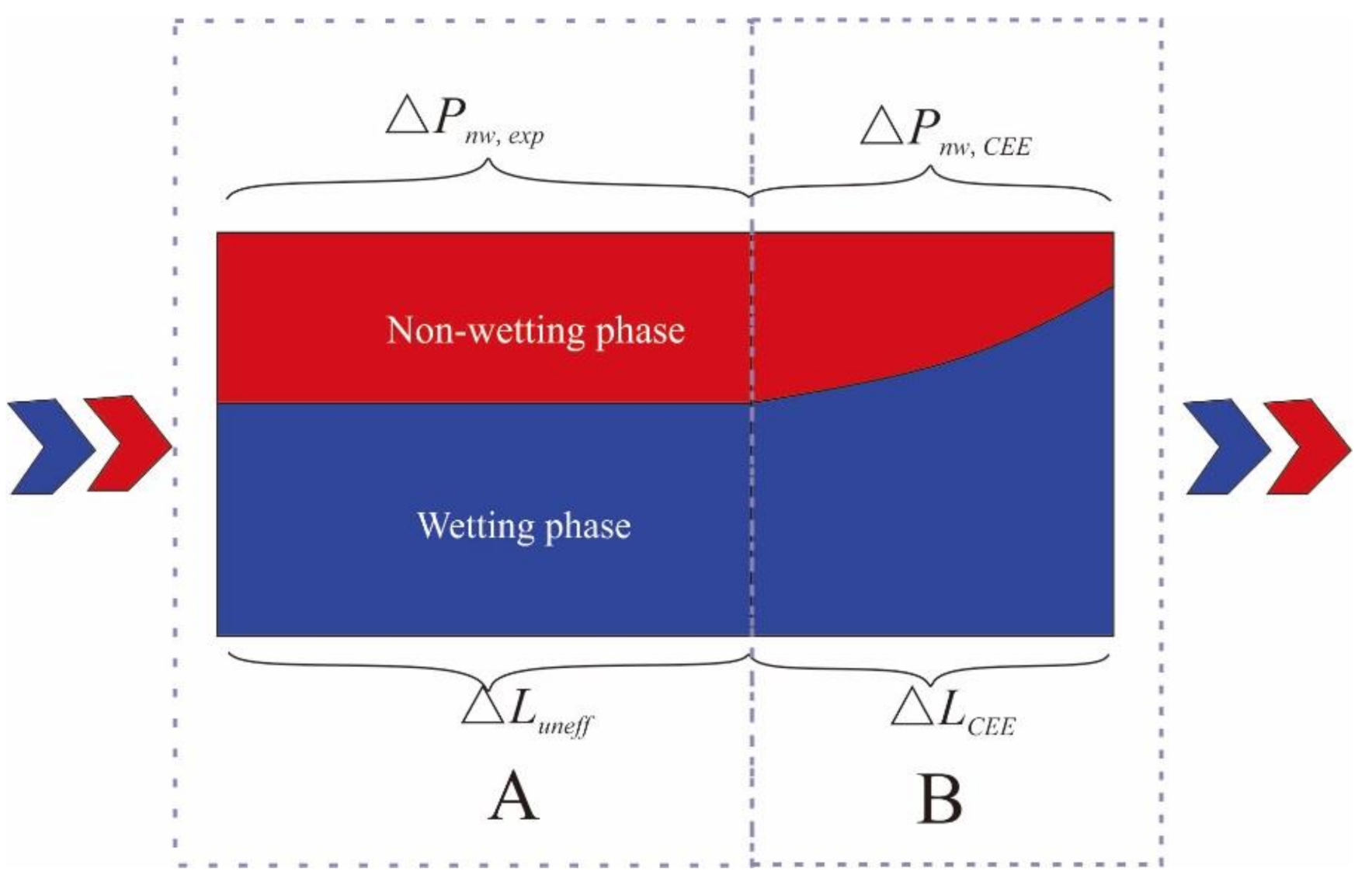
| Characteristic | This type of correction method is more dependent on the selection of the empirical formula. | This method corrects the capillary end effect by constructing the pressure relationship between the region affected by the capillary end effect and the region not affected by the capillary end effect inside the core. |
| Advantage | This kind of method requires once unsteady-state relative permeability experiments. | This type of method does not rely on the selection of the relative permeability formula, so the correction result is more accurate. |
| Disadvantage | The correction results of this type of method are diversified and accurate correction data cannot be obtained because the empirical formula of the correlation is more diversified. | This kind of method requires a large number of steady-state relative permeability experiments. |
| Reference number | [23,24,25,26,27,28] | [30,31] |
| Core Number | Length/cm | Diameter/cm | Area/cm2 |
|---|---|---|---|
| 60-1 | 7.990 | 2.540 | 1.613 |
| Porosity/% | Absolute permeability/D | Dry weight/g | Wet weight/g |
| 19.778 | 0.0631 | 84.739 | 93.027 |
| Core Number | Component Content (%) | ||||
|---|---|---|---|---|---|
| Quartz | Potash Feldspar | Plagioclase | Calcite | Dolomite | |
| 60-1 | 68 | 1 | 5 | 25 | 1 |
| Pyrite | Barite | Anhydrite | Analcite | Hematite | |
| 0 | 0 | 0 | 0 | 0 | |
| Experiment Number | Proportion of Injected Liquid | Total Flow Rates/(mL/min) | ||
|---|---|---|---|---|
| 1 | 1:10 | 0.3 | 0.027 | 0.273 |
| 2 | 1:10 | 0.6 | 0.055 | 0.545 |
| 3 | 1:10 | 1.1 | 0.100 | 1.000 |
| 4 | 1:10 | 2.2 | 0.200 | 2.000 |
| 5 | 1:10 | 1.1 | 0.100 | 1.000 |
| 6 | 5:01 | 0.3 | 0.250 0.500 | 0.050 0.100 |
| 7 | 5:01 | 0.6 | ||
| 8 | 5:01 | 1.1 | 0.917 1.833 | 0.183 0.367 |
| 9 | 5:01 | 2.2 | ||
| 10 | 1:10 | 1.1 | 0.100 | 1.000 |
| 11 | 1:05 | 0.3 | 0.050 0.100 | 0.250 0.500 |
| 12 | 1:05 | 0.6 | ||
| 13 | 1:05 | 1.1 | 0.183 0.367 | 0.917 1.833 |
| 14 | 1:05 | 2.2 | ||
| 15 | 1:10 | 1.1 | 0.100 | 1.000 |
| Experiment Number | Proportion of Injected Liquid | Pressure Drop/MPa | Water Saturation |
|---|---|---|---|
| 3 | 1:10 | 7.420 | 0.420 |
| 5 | 1:10 | 7.924 | 0.412 |
| 10 | 1:10 | 7.991 | 0.437 |
| 15 | 1:10 | 7.210 | 0.457 |
| Core Number | |||||
|---|---|---|---|---|---|
| - | 4.61 | 3.77 | 11.16 | 13.5 | 9.9 |
| Experiment Number | |||
|---|---|---|---|
| 1 | 0.08 | 0.07 | 3.95 |
| 2 | 0.08 | 4.82 | |
| 3 | 0.25 | 13.51 | |
| 4 | 0.50 | 26.55 | |
| 5 | 0.02 | 0.18 | 6.46 |
| 6 | 0.25 | 8.42 | |
| 7 | 0.42 | 13.31 | |
| 8 | 0.83 | 25.53 |
| Number | |||
| 1 | 2.87 | 3.18 | 1.20 |
| 2 | 2.87 | 2.54 | 1.20 |
| 3 | 2.87 | 0.85 | 1.20 |
| 4 | 2.87 | 0.42 | 1.20 |
| 5 | 6.04 | 4.25 | 1.22 |
| 6 | 6.04 | 3.11 | 1.22 |
| 7 | 6.04 | 1.87 | 1.22 |
| 8 | 6.04 | 0.93 | 1.22 |
| Number | ||||
|---|---|---|---|---|
| 1 | 3.95 | 0.0054 | 0.1510 | 0.048 |
| 2 | 4.82 | 0.0067 | ||
| 3 | 13.51 | 0.0202 | 0.1510 | 0.048 |
| 4 | 26.55 | 0.0404 | ||
| 5 | 6.46 | 0.0148 | 0.2685 | 0.110 |
| 6 | 8.42 | 0.0202 | ||
| 7 | 13.31 | 0.0337 | 0.2685 | 0.110 |
| 8 | 25.53 | 0.0674 |
| Number | |||
|---|---|---|---|
| 1 | 0.155 | 0.155 | 3.53 × 10⁻⁶ |
| 2 | |||
| 3 | 0.155 | 6.8 × 10⁻⁵ | |
| 4 | |||
| 5 | 0.276 | 0.155 | 9.4 × 10⁻⁵ |
| 6 | |||
| 7 | 0.276 | 2.5 × 10⁻⁵ | |
| 8 |
Publisher’s Note: MDPI stays neutral with regard to jurisdictional claims in published maps and institutional affiliations. |
© 2021 by the authors. Licensee MDPI, Basel, Switzerland. This article is an open access article distributed under the terms and conditions of the Creative Commons Attribution (CC BY) license (https://creativecommons.org/licenses/by/4.0/).
Share and Cite
Li, Y.; Wang, S.; Kang, Z.; Yuan, Q.; Xue, X.; Yu, C.; Zhang, X. Research on the Correction Method of the Capillary End Effect of the Relative Permeability Curve of the Steady State. Energies 2021, 14, 4528. https://doi.org/10.3390/en14154528
Li Y, Wang S, Kang Z, Yuan Q, Xue X, Yu C, Zhang X. Research on the Correction Method of the Capillary End Effect of the Relative Permeability Curve of the Steady State. Energies. 2021; 14(15):4528. https://doi.org/10.3390/en14154528
Chicago/Turabian StyleLi, Yanyan, Shuoliang Wang, Zhihong Kang, Qinghong Yuan, Xiaoqiang Xue, Chunlei Yu, and Xiaodong Zhang. 2021. "Research on the Correction Method of the Capillary End Effect of the Relative Permeability Curve of the Steady State" Energies 14, no. 15: 4528. https://doi.org/10.3390/en14154528
APA StyleLi, Y., Wang, S., Kang, Z., Yuan, Q., Xue, X., Yu, C., & Zhang, X. (2021). Research on the Correction Method of the Capillary End Effect of the Relative Permeability Curve of the Steady State. Energies, 14(15), 4528. https://doi.org/10.3390/en14154528