Modified Flower Pollination Algorithm for Global Optimization
by
 and
and
Mohamed Abdel-Basset
1, 
Reda Mohamed
1,
Safaa Saber
1,
S. S. Askar
2 and
Mohamed Abouhawwash
3,4,*
1
Department of Computer Science, Faculty of Computers and Informatics, Zagazig University, Zagazig 44519, Egypt
2
Department of Statistics and Operations Research, College of Science, King Saud University, Riyadh 11451, Saudi Arabia
3
Department of Mathematics, Faculty of Science, Mansoura University, Mansoura 35516, Egypt
4
Department of Computational Mathematics, Science, and Engineering (CMSE), College of Engineering, Michigan State University, East Lansing, MI 48824, USA
*
Author to whom correspondence should be addressed.
Mathematics 2021, 9(14), 1661; https://doi.org/10.3390/math9141661
Submission received: 27 May 2021
/
Revised: 28 June 2021
/
Accepted: 30 June 2021
/
Published: 15 July 2021
Abstract
:In this paper, a modified flower pollination algorithm (MFPA) is proposed to improve the performance of the classical algorithm and to tackle the nonlinear equation systems widely used in engineering and science fields. In addition, the differential evolution (DE) is integrated with MFPA to strengthen its exploration operator in a new variant called HFPA. Those two algorithms were assessed using 23 well-known mathematical unimodal and multimodal test functions and 27 well-known nonlinear equation systems, and the obtained outcomes were extensively compared with those of eight well-known metaheuristic algorithms under various statistical analyses and the convergence curve. The experimental findings show that both MFPA and HFPA are competitive together and, compared to the others, they could be superior and competitive for most test cases.
1. Introduction
In recent decades, meta-heuristic optimization algorithms have widely interfered in several fields, tackling numerous optimization problems, especially engineering problems, due to fabulously avoiding stagnation in local optima, with high convergence speed in the right direction of the near-optimal solution [1]. The meta-heuristic algorithms have been classified into four categories according to the inspiration nature: evolutionary algorithms, physics-based algorithms, swarm-based algorithms, and human-based algorithms. The first category, called evolution-based algorithms, mimics biological evolution based on reproduction, mutation, recombination, and selection to produce new offspring stronger than their parents. The most population evolutionary algorithms which have been significantly applied for various optimization problems are genetic algorithms (GA) [2], evolution strategy (ES) [3], genetic programming (GP) [4], probability-based incremental learning (PBIL) [5], and biogeography-based optimizer (BBO) [6].
The physics-based algorithms have been simulating the laws of physics for proposing other algorithms with various behaviors, in the hope of coming true better outcomes; some of those algorithms are simulated annealing (SA) [7], Big-Bang Big-Crunch (BBBC) [8], Gravitational Search Algorithm (GSA) [9], Small-World Optimization Algorithm (SWOA) [10], Curved Space Optimization (CSO) [11], Galaxy-based Search Algorithm (GbSA) [12], Charged System Search (CSS) [13], Artificial Chemical Reaction Optimization Algorithm (ACROA) [14], Ray Optimization (RO) [15], Equilibrium Optimizer (EO) [16], Billiards-inspired optimization algorithm (BOA) [17], and Black Hole (BH) [18].
The social behavior-inspired algorithms, or swarm-based algorithms, as the third category, have been developed to model the social behaviors of birds and animals; those algorithms involve Particle Swarm Optimization (PSO) [19], Whale Optimization Algorithm (WOA) [1], Harris Hawks algorithm (HHA) [20], Marine Predators Algorithm (MPA) [21], Slime Mold Algorithm (SMA) [22], Ant Colony Optimization (ACO) [23], Grey Wolf Optimizer (GWO) [24], Cuckoo Search (CS) [25], Bat Algorithm (BA) [26], flower pollination algorithm (FPA) [27], and several others [28,29,30,31,32,33,34,35,36,37,38,39,40].
The last category, called human-based algorithms, has worked on emulating human behaviors, for proposing other algorithms with different methodology; including Teaching Learning Based Optimization(TLBO) [41], Harmony search (HS) [42], League Championship Algorithm (LCA) [43], Group Counseling Optimization (GCO) [44,45], Mine Blast Algorithm (MBA) [46], Seeker Optimization Algorithm (SOA) [47], Soccer League Competition (SLC) algorithm [48,49], Firework Algorithm [50], and many others [51].
The significant successes achieved by metaheuristic algorithms have given them the first rank as optimization models for tackling several optimization problems in a reasonable time [52]. One of the most popular optimization problems tackled by those optimization algorithms is nonlinear equation systems (NESs).
Nonlinear equation systems (NESs) have significantly arisen in engineering and science fields and solving those systems has recently attracted the attention of several researchers for finding effective optimization methods [53,54,55]. The optimization methods proposed for tackling the NESs have been divided into two categories: metaheuristic and classical. The metaheuristic techniques won significant interest over the classical ones due to averting being stuck in local minima, accelerating the convergence speed, and independence of the initial guess, in addition to fulfilling better outcomes in a reasonable time as discussed before. Several papers apply the metaheuristic algorithms: human-, evolution-, swarm-, and physics-based, for tackling the NESs, as discussed in the next section. The mathematical model of the NESs are described as:
where D refers to the number of dimensions, n determines the number of equations, and x involves the solution to the NESs. As shown in Equation (1), the NESs consists of more than one objective function and, hence, the metaheuristic algorithms designed to deal with the problem with a single objective are not able to solve them. Therefore, the NESs will be converted into a single objective to be solvable by the metaheuristic algorithms using the following formula:
The flower optimization algorithm (FPA) proposed for tackling the global optimization based on mimicking the pollination process of flowers have had an effective performance for tackling several optimization problems [27,56,57,58,59,60,61], but unfortunately, its performance still substantially suffers from stagnation in local minima because of the inability to explore several regions within the search space during the optimization process, in addition to having low convergence speed, which makes the classical FPA consume several iterations for searching better solutions within unpromising regions. Broadly speaking, the classical FPA was evaluated using 10 mathematical test functions under a population size of 25 and maximum iteration reaching 10,840; this is considered a significant rate to be consumed for coming to the desired outcomes. Furthermore, the authors in [56] hybridized the classical FPA with the clonal selection algorithm (CSA) to solve 23 global test functions. This work was based on improving the local search of the classical FPA to avoid being stuck in local minima, and to reach better outcomes. In our opinion, that hybridization between two algorithms, to mix the advantages of each one to overcome their owning disadvantages, is considered a good alternative, but that might be sometimes ineffective because of difficulty in finding two or more algorithms completing each other to reach better outcomes. As an easier alternative, we see that the structure of the classical algorithms needs to be redesigned differently to create various updating schemes, working on exploring several regions within the search space for reaching better outcomes without wasting the iterations useless.
Therefore, a new modified FPA (MFPA) is proposed in this paper to overcome all those aforementioned problems, by building an effective mathematical model based on effectively hybridizing various updating schemes to enable this modified algorithm of adapting itself during looking for the solutions to the optimization problem. This modified algorithm could overcome the standard one for all 23 well-known unimodal and multimodal test functions and 27 NESs. However, unfortunately, it still suffers from a defect in its exploration operator, which prevents it from reaching better outcomes for some test functions compared to the competing algorithms.
Therefore, a well-established evolutionary algorithm known as differential evolution (DE) has been successfully applied to tackling several optimization problems, either continuous or discrete ones, and enjoyed with various updating schemes. One of those schemes, having a high ability for the exploration, is “DE/rand/1”, which explores the regions around one selected randomly from the population [62]. There are several DE variants based on various updating schemes or hybridization between DE, and some effective techniques have been extensively applied to tackle global optimization [63,64,65,66,67,68,69,70,71,72,73]. Since our proposed, MFPA suffers from a problem in the exploration operator, and the DE’s updating scheme “DE/rand/1”, have more direction to the exploration operator than the exploitation. DE is integrated with MFPA to propose a new variant called HFPA, balancing between the exploration and exploitation for preserving the population diversity to avoid being stuck into the local minima, and moving accurately toward the best-so-far solution to reduce the time-consuming fitness function evaluations. After validation and comparison on 23 well-known unimodal and multimodal test functions, HFPA has superior outcomes compared to the rival algorithms, with success rates reaching 78% and 70% in best and average cases, also outperforming MFPA, which has percentages of 61% and 52% as the second-best one.
Finally, our proposed algorithms: HFPA and MFPA have further investigated 27 NESs, and compared with some recent (and well-established) optimization algorithms, which show that those proposed algorithms are better with outperformance rate, reaching 100% and 81% in the best case, and 67% and 37% in the average case. It is concluded—based on the experimental findings—that HFPA is better than all competing algorithms and MFPA for both global optimization and NESs; thus, it is a strong alternative to tackle those two types of optimization problems. Briefly, this paper presents the following contributions:
- ➢
- Proposes a modified variant of the classical FPA, namely MFPA, with various updating schemes to tackle both global optimization and NESs.
- ➢
- Improves the exploration operator of MFPA using the DE with the “DE/rand/1” scheme to propose a new hybrid variant, called HFPA, with strong attributes.
- ➢
- The experimental findings show that HFPA has superior performance for tackling global optimization and NESs compared to eight rival algorithms and MFPA.
The structure of this paper is depicted in Figure 1: Section 2 describes works done previously on tackling the NESs. Section 3 describes the standard algorithms: FPA and DE. Section 4 shows our proposed algorithms, explaining them clearly and effectively. Section 5 exposes various experiments and presents some discussions. Finally, Section 6 presents our conclusions and future work.
2. Literature Review: NESs
As aforementioned—NESs are a hot research area that have attracted the attention of researchers (in terms of proposing an optimization model that could optimally solve them in a reasonable time). Therefore, researchers have significantly moved towards metaheuristic algorithms as a strong alternative to the classical ones to tackle NESs. Some of the metaheuristic algorithms proposed for tackling the NESs are reviewed next.
Ramadas, G.C. and E.M.d.G [74] have employed some variants of the harmony search algorithm to tackle NESs. Furthermore, the social emotion optimization algorithm (SEOA) was recently published with some improvements to develop a new variant, namely HSEOA, avoiding being stuck in local optima in order to reach better outcomes [75]. In addition, another method based on the multi-crossover real-coded genetic algorithm was proposed to tackle NESs, and was compared to some evolutionary algorithms to show its superiority [76]. Furthermore, Grosan, C., et al. [77] dealt with this problem as a multi-objective one, where each function represented an objective and tried to find the non-dominated solution, which minimizes all of the test functions together.
In the same context, a new efficient variant of the genetic algorithm (GA) improved, using the symmetric and harmonious individuals and elitism way to improve the population diversity and the convergence speed, respectively [78]. The particle swarm optimization improved using a conjugate direction (CD) method, and was developed to propose a new variant, namely CDPSO, overcoming the optimization problems with high dimensions [79]. Moreover, in [80], the PSO was used as a technique for tackling NESs as suggested to overcome the disadvantages of the classical methods, e.g., Newton’s method. A new NES technique based on the modified firefly algorithm was employed to deal with the problems with multiple roots [81]. In [82], another NES approach, named parallel elite-subspace evolutionary algorithm (PESEA), was proposed to tackle NESs in a reasonable time.
The grasshopper optimization algorithm (GOA) and genetic algorithm (GA) were effectively integrated to produce a hybrid variant, namely hybrid-GOA-GA, which could efficiently tackle the NESs [83]. This hybrid variant was validated using eight benchmark problems with different applications and its outcomes were compared with some of the state-of-the-art outcomes, in terms of computational costs, final results, and convergence speed. The experimental outcomes show its effectiveness for all of these terms. Furthermore, differential evolution (DE) was improved using two methods: a new mutation operation strategy and a restart technique to preserve the population diversity and avoid being stuck in local minima, which had to, by the standard DE, suggest a new variant, namely DE-R, to accurately solve the NESs. DE-R was validated using different real-world problems and compared with some recently proposed methods to show its superiority. In terms of the convergence speed and accuracy, DE-R was better.
A new hybrid algorithm was recently employed for solving NESs [84]. This hybrid algorithm, called DEMBO, was based on integrating the differential evolution (DE) algorithm into the monarch butterfly optimization (MBO) to overcome its defects confined to time-consuming fitness functions and falling in local minima. This algorithm was evaluated using nine unconstrained optimization problems and eight NESs, and compared to some state-of-the-art algorithms. The experimental findings demonstrate its superiority over the competing ones. In [85], a framework based on both grey wolf optimizer and multi-objective particle swarm optimization was proposed to tackle the NESs. This framework could be more effective compared to some of the classical and metaheuristic techniques. The differential evolution unified with a method, known as the Powell conjugate direction method, to avert stagnation in local minima was suggested, to propose a system called DE-Powell for tackling the NESs [86]. DE-Powell could be more effective compared to several existing algorithms when solving nine NESs.
The cuckoo search algorithm and the niche strategy have been combined to propose a strong variant called the niche cuckoo search algorithm (NCSA) for solving NESs [87]. NCSA has been benchmarked using 20 well-known mathematical test functions and some NESs, and compared to three well-established metaheuristic algorithms, such as chaos gray-coded genetic algorithm, classical genetic algorithm, and standard cuckoo search algorithm, showing that this algorithm is more adaptable compared to the other for solving the NESs. A hybrid algorithm, based on incorporating the cuckoo search (CS) with the particle swarm optimization (PSO), to overcome the huge function evaluations required by CS and local minima as the defect of the PSO, has been proposed in a variant named CSPSO to tackle the NESs [88]. CSPSO was benchmarked by some NESs and 28 CEC2013 benchmark functions to show its efficiency, as well as compared with some existing algorithms to measure its efficiency.
The bat algorithm, improved by a differential operator and Levy flight strategy, to accelerate the convergence speed and avoid local minima, respectively, were proposed; this improved variant was named DLBA [89]. Fourteen typical test functions and an NES have been employed for benchmarking the efficiency of the proposed algorithm compared to some other optimization algorithms. The experimental findings show the effectiveness of DLBA for finding better solutions than all competing ones.
In [90], a comparative study among the various variant of the genetic algorithms, in addition to the classical methods, was performed to see which one is better for solving the system of equations. The experimental results of this study showed that a modified GA variant was the best. The grey wolf optimizer was efficiently combined with the DE to produce a new variant called GWO-DE, with strong characteristics, such as avoiding getting stuck in local minima and accelerating the convergence speed, for solving the NESs [91]. The experimental findings, as mentioned by the authors, proved the efficacy of GWO-DE for tackling most of the NESs, compared to the existing optimization techniques. There are several other approaches proposed for tackling the NESs [92,93,94,95].
3. Overview of Used Metaheuristic Techniques
3.1. Flower Pollination Algorithm (FPA)
Yang, X.-S. [27] proposed a nature-inspired metaheuristic optimization algorithm called the flower pollination algorithm (FPA), based on mimicking the pollination process of flowers. There are two kinds of pollination: self-pollination and cross-pollination. In self-pollination, the fertilization process is performed between the flowers of the same types, where the pollen from one flower goes to fertilize another similar one. Cross-pollination is related to transferring the pollen for long distances between different plants, by insects, such as birds, bees, and bats. It is worth mentioning that some insects tend to visit some flowers without the others, in a phenomenon called flower constancy. Generally, the flower pollination process could be described in the following rules:
- Biotic and cross-pollination can be defined as global pollination used to explore the regions of the search space for finding the most promising regions. This stage is based on the levy distribution.
- The abiotic self-pollination describes the local pollination utilized to exploit the regions around the current solution for accelerating the convergence speed.
- The flower constancy property can be regarded as a reproduction ratio that is proportional to the degree of similarity between two flowers.
- Local pollination has a slight advantage in comparison to global pollination due to the physical proximity and wind. In specific, the local and global pollinations are controlled by a control variable P having a value between 0 and 1.
The mathematical model of global pollination and flower constancy is based on involving the fittest insect through the ones that travel for long distances, which is described as follows:
where t indicates the current iteration, is the current position of the ith solution, is the best-so-far solution, l is a step generated based on the levy distribution, is the step size scaling factor, and express the next position. While the mathematical model of local pollination is described as follows:
where is a variable involving a random value generated at the interval of 0 and 1 based on the uniform distribution. and are two solutions selected randomly from the current population.
3.2. Differential Evolution
Storn, R.J.T.r. [96] proposed a population-based optimization algorithm named differential evolution (DE), similar to genetic algorithms, in terms of the mutation, crossover, and selection operators. The differential evolution before starting the optimization process initializes a number of individuals with D dimensions for each one , where NP is the individuals number and called also as population size and D is the dimension size, within the search space of an optimization problem. Afterwards, the mutation and crossover operators have been applied to explore the search space for finding better solutions as described below.
3.2.1. Mutation Operator
This operator has been employed by DE to generate a mutant vector, namely , for each individual , called as target vector, in the population. The mutant vector is generated using the mutation strategy described below:
where is a random solution selected randomly from the population at generation t. F is a positive scaling factor.
3.2.2. Crossover Operator
After generating the mutant vector , the crossover operator has been employed to generate a trial vector based on the current position of the individual and its corresponding mutant one, according to a crossover probability (CR). This crossover operation is described as follows:
is a random integer generated between 1 and D, indicates the current dimension, and is a constant value predefined between 0 and 1 to determine the percentage of the dimensions copied to the trial vector from the mutant one.
3.2.3. Selection Operator
Finally, the selection operator is used to evaluate the trial vector and the current one and the fittest one is used at the next generation. In general, the selection process for a minimization problem is expressed using the mathematical formulation as such:
where f(.) indicates the objective function or often known as the fitness function.
4. Proposed Algorithm: Hybrid Modified FPA (HMFPA)
The steps used to build the proposed algorithm, developed for solving the global optimization and NESs, are described in this section, and involve initialization, evaluation, modification, and comprehensive algorithm.
4.1. Initialization
Before beginning the optimization process, NP solutions will be distributed within the lower bound and upper bound vectors of the optimization problem using the following formula:
where are the upper and lower bound vectors, is a vector consisting of D cells having values generated randomly between 0 and 1. Afterward, those initialized solutions will be evaluated using Equation (2) to find the best-so-far solution used at the next generation for updating the current population in the hope of exploring a better one.
4.2. Modified Flower Pollination Algorithm (MFPA)
4.2.1. Global Pollination
The classical FPA has designed a mathematical model for the global pollination, which is based on transferring the pollens among the plants by insects, based on updating the current position in a reverse direction to the best-so-far solution, , to take the pollens for a long distance. However, this involves some defects, mentioned next, which might affect the performance of the FPA. Since the main goal of this stage takes the pollen a long distance to fertilize other plants, it is not essential to always move the current position in the reverse direction into the best-so-far, because updating using various schemes, which might be combined in an effective manner to take the pollen to several regions, involving various plants within the search space, might significantly affect the optimization process. Therefore, three various updating schemes swapped effectively to take the pollen to several regions within the optimization process are mathematically described as follows. The first updating scheme is based on relating the current position to each search agent with the current iteration to help the algorithm gradually explore various regions around the current solution within the search space, even reaching the end of the iteration. In this case, the optimization process will focus on a local search around this current solution in the hope of finding a better solution. Generally, this updating scheme is modeled as follows:
where indicates the maximum iteration, a is a distance control factor to determine the distance around the current position to be explored. The second updating scheme is searching around the best-so-far solution based on two-step sizes: the first one will take the algorithm in a reverse direction to the best-so-far solution, while the other works on improving this direction to be close to the best-far solution, to promote the exploitation operator, or further, to strengthen the exploration operator. The mathematical model of this scheme is described as follows:
where and are two solutions randomly selected from the population at iteration t, while is a numerical value generated between 0 and 1 under the uniform distribution. Finally, the third updating scheme is based on exploring the regions between the current best-so-far position and its negative one, based on the uniform distribution, to avoid being stuck in local minima, as modeled mathematically below:
U indicates a uniform distribution method that takes the lower endpoints and upper endpoint as inputs and return a vector involves random values generated in-between; where is a value created randomly between 0 and 1. The swapping between those three updating scheme is achieved as described by the following equation to balance between the implementation of the following updating scheme and the other two, as an attempt to balance between the exploration and exploitation capability:
where r, r1, and r2 are numerical values generated randomly between 0 and 1.
4.2.2. Local Pollination
Regarding modification to the mathematical model at this stage—our idea was based on designing one using two various schemes that are exchanged using a probability of 0.5 to involve balance between them. The first one searches around the current position scaled according to the current iteration, to promote the searchability of the algorithm within the search space, to avoid being stuck in local minima. The second searches around the best-so-far solution, and is also scaled according to the current iteration to improve the exploitation operator, to accelerate the convergence speed in the right direction of the near-optimal solution.
where and are two solutions selected randomly from the population, and is a random number generated between 0 and 1. Finally, Algorithm 1 shows the steps of modified FPA (MFPA) and the same steps depicted in Figure 2.
| Algorithm 1 The Steps of MFPA |
| 1. Initialization step. |
| 2. Evaluation. |
| 3. while (t < ) |
| 4. For (I = 1: NP) |
| 5. : create a random number between 0 and 1. |
| 6. if (r > p) |
| 7. Update using Equation (15) |
| 8. Else |
| 9. Update using Equation (18) |
| 10. End if |
| 11. End for |
| 12. Evaluation step. |
| 13. t = t + 1; |
| 14. end while |
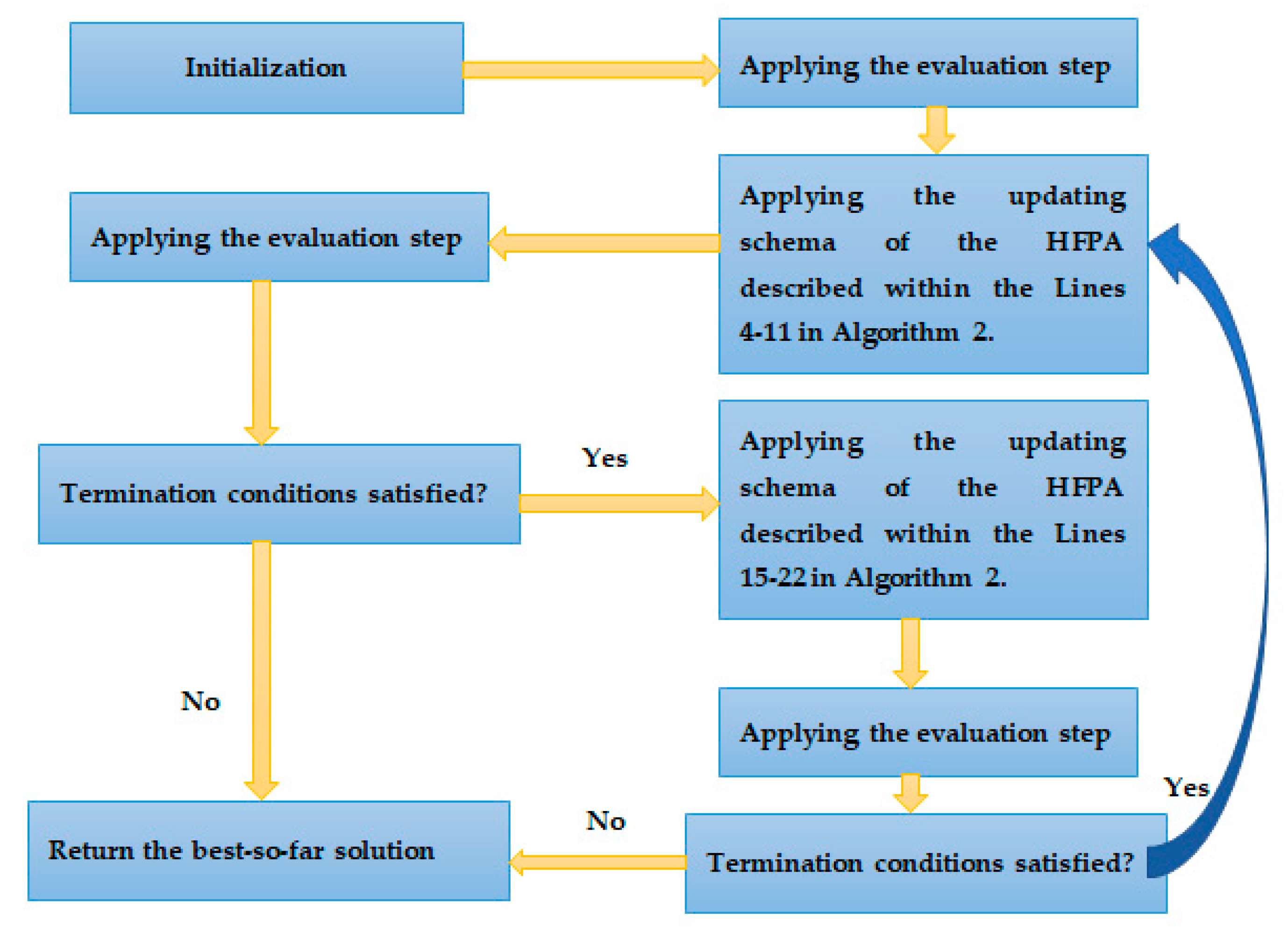
4.3. Hybridization of MFPA with DE(HFPA)
Unfortunately, MFPA still suffers from a lack of population diversity; this will pull the algorithm into the local minima and, hence, it cannot get to the near-optimal solution. Therefore, the DE has been effectively integrated into MFPA with a probability , picked experimentally, as shown in the experiments section later, even taking the algorithm into other regions, preserving the population diversity for achieving better outcomes. Finally, the steps of integrating MFPA with DE are listed in Algorithm 2, and its framework is described in Figure 3.
| Algorithm 2 The Steps of HFPA |
| 1. Initialization step. |
| 2.Evaluation. |
| 3.while (t < ) |
| 4. For (i = 1: NP) |
| 5. : create a random number between 0 and 1. |
| 6. if (r > p) |
| 7. Update using Equation (15) |
| 8. Else |
| 9. Update using Equation (18) |
| 10. End if |
| 11. End for |
| 12. Evaluation step. |
| 13. t = t + 1; |
| 14. /// Applying differential evolution |
| 15. if r< |
| 16. For (i=1: NP) |
| 17. Creating a mutant vector for using Equation (5) |
| 18. Applying crossover operator. |
| 19. Applying selection operator |
| 20. End for |
| 21. t = t + 1; |
| 22. End if |
| 23. end while |
5. Outcomes and Discussion
This section assesses the performance of the proposed algorithm using two independent experiments: the first one is based on checking its performance to search for the near-optimal solution for 23 well-known mathematical test functions, and the second will employ this, proposed for estimating the roots of 27 common NESs. Specifically, this section is organized as follows:
- ➢
- Section 5.1 shows the parameter settings and benchmark test functions.
- ➢
- Section 5.2 presents validation and comparison under 23 global optimization problems.
- ➢
- Section 5.3 presents validation and comparison under 27 NESs.
5.1. Parameter Settings
The proposed algorithm has been compared with eight well-known, recently-published metaheuristic algorithms, such as equilibrium optimizer (EO, 2020) [16], marine predators algorithm (MPA, 2020) [21], particle swarm optimization (PSO) [19], differential evolution (DE) [96], horse herd optimization algorithm (HOA, 2020) [97], slime mold algorithm (SMA, 2020) [22], and Runge Kutta based optimizer (RUN, 2021) [98]. Those algorithms have been implemented in the MATLAB platform under the same parameter values found in the cited papers, which are the original study for those algorithms.
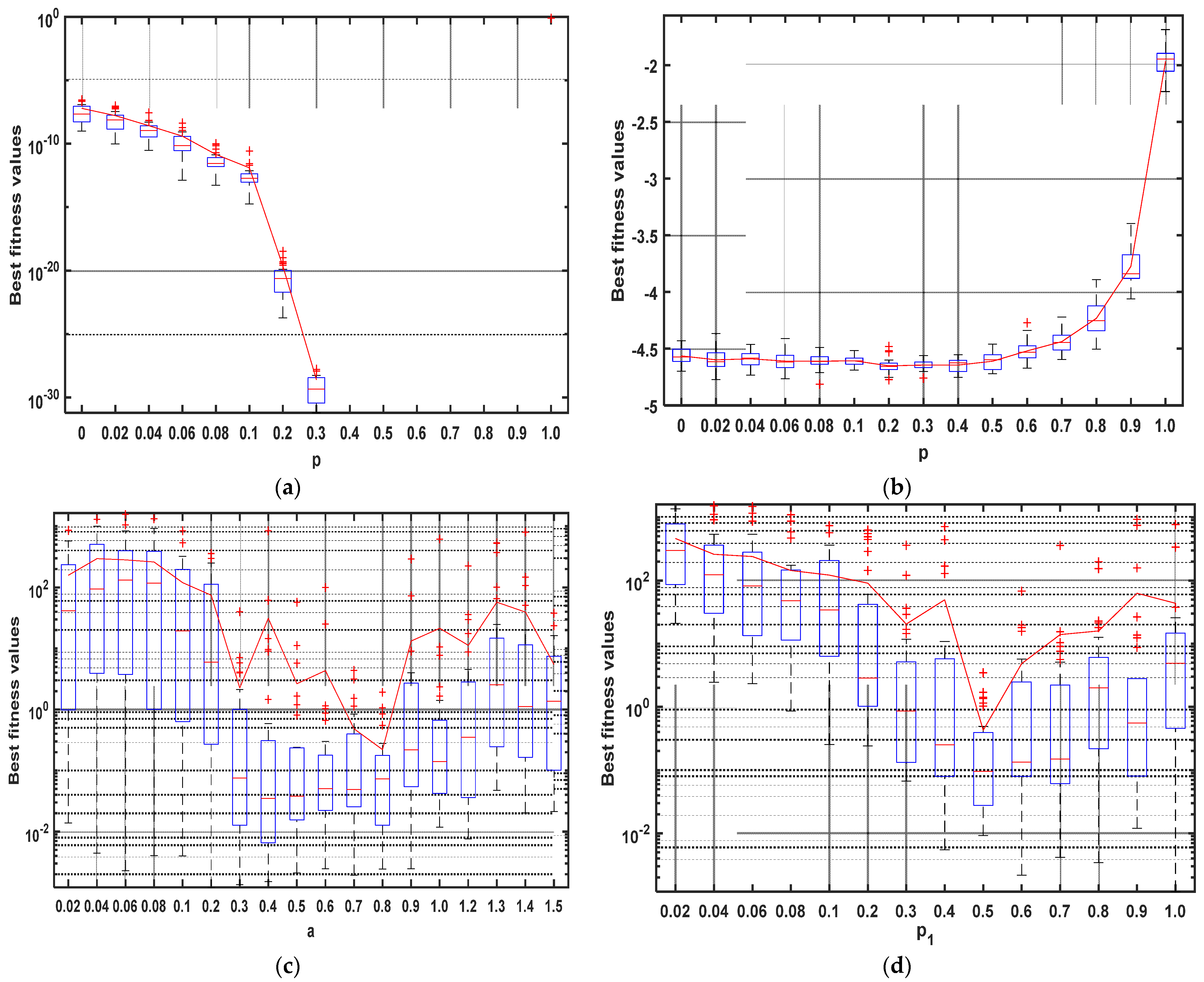
Regarding the parameters of each compared algorithm, they were assigned at the implementation, as cited in the published papers. However, the proposed algorithms: MFPA and HFPA have three effective parameters, which need to be optimally picked to maximize their performances, those parameters are p, , and . After executing different experiments with different values for each parameter on different test functions, it is obvious that the best value for p is 0.4, as shown in Figure 4a,b. The best for the parameters a and are of 0.8 and 0.5, as shown in Figure 4c,d. Regarding the parameter for the proposed, it is set to 0.5 to increase the step size for increasing the exploration operator, while the parameters CR and F are set to 0.9 and 0.5, respectively, as described in [99]. All algorithms were executed 30 independent times with a population size of 30 and a maximum iteration of 500 under the same machine to ensure a fair comparison.
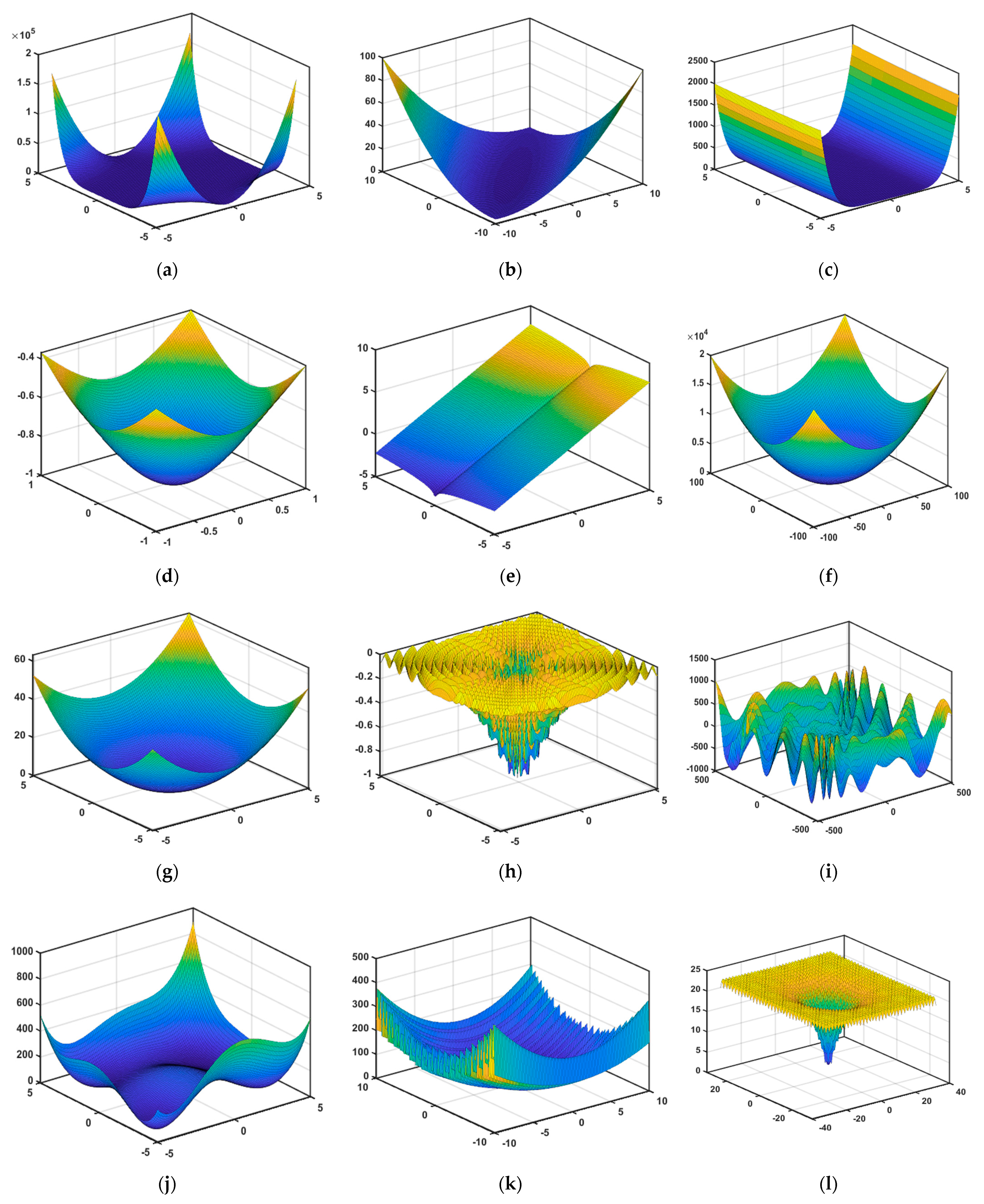
The algorithms are here compared based on estimating the optimal value for two benchmarks: the first one consists of eight well-known unimodal mathematical test functions and 15 multimodal ones, as described in Table 1, which consists of four columns: the first one called “Name” mentions the function name, the second labeled “Formula: shows the mathematical equation of each function, the third labeled “D” carries the number of dimensions, and the last labeled “R” involves the search area of each function. The second benchmark involves 28 widely used NESs, defined in Table 2. The landscape of the unimodal and multimodal functions are depicted in Figure 5 to display the difference between the two.
5.2. Comparison of the Global Optimization
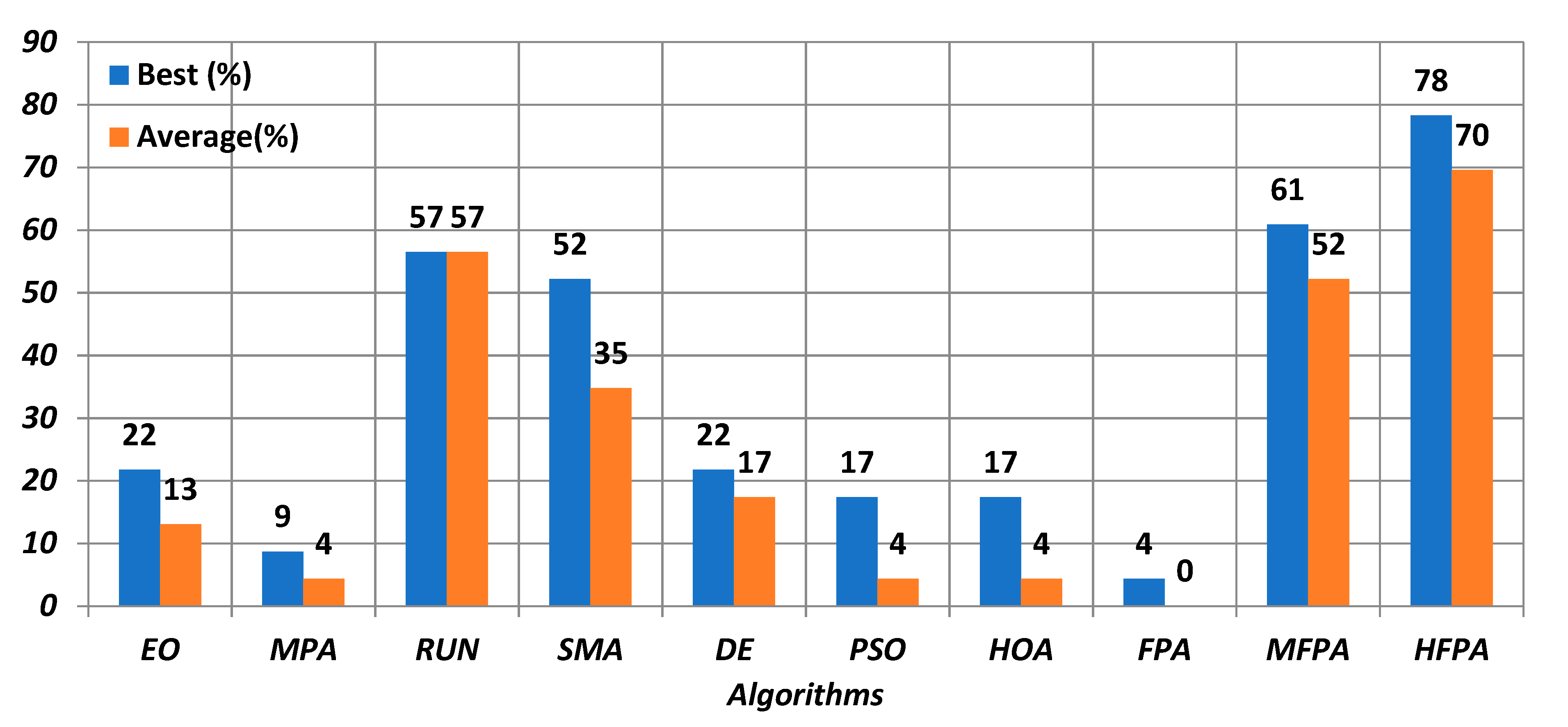
This section is presented to compare the performance of the standard FPA, MFPA, and HFPA together, and with seven well-known swarm and evolutionary algorithms to see how far our modification to the standard FPA could positively affect its performance for solving 23 well-known unimodal and multimodal functions. Due to the stochastic nature of these algorithms, they are executed 30 independent times, and the best, Avg, worst, and standard deviation (SD) of the fitness values obtained by each one were calculated and exposed in Table 3 and Table 4. Inspecting Table 3 and Table 4 shows that both MPFA and HFPA could outperform the classical FPA for all used test functions and this affirms that our modification could aid the standard in reaching other regions not reachable by this classical one. Not only could HFPA outperform the standard one, but it could also be superior and competitive with the rival algorithms and MFPA for 16 out of 23 test function, with a percentage up to 70%, as shown in Figure 6 in all independent runs. Moreover, for the other seven test functions, it could reach less value in the best case for two with a total percentage of 78%, as depicted in Figure 6, and its performance was significantly converged for the other ones. This superiority achieved by HFPA is due to preserving the population diversity among the individuals along the optimization process and this helps it avoid being stuck in local minima, which prevents it from reaching better outcomes. Based on that, HFPA is a strong alternative metaheuristic algorithm to the existing ones for tackling optimization problems.
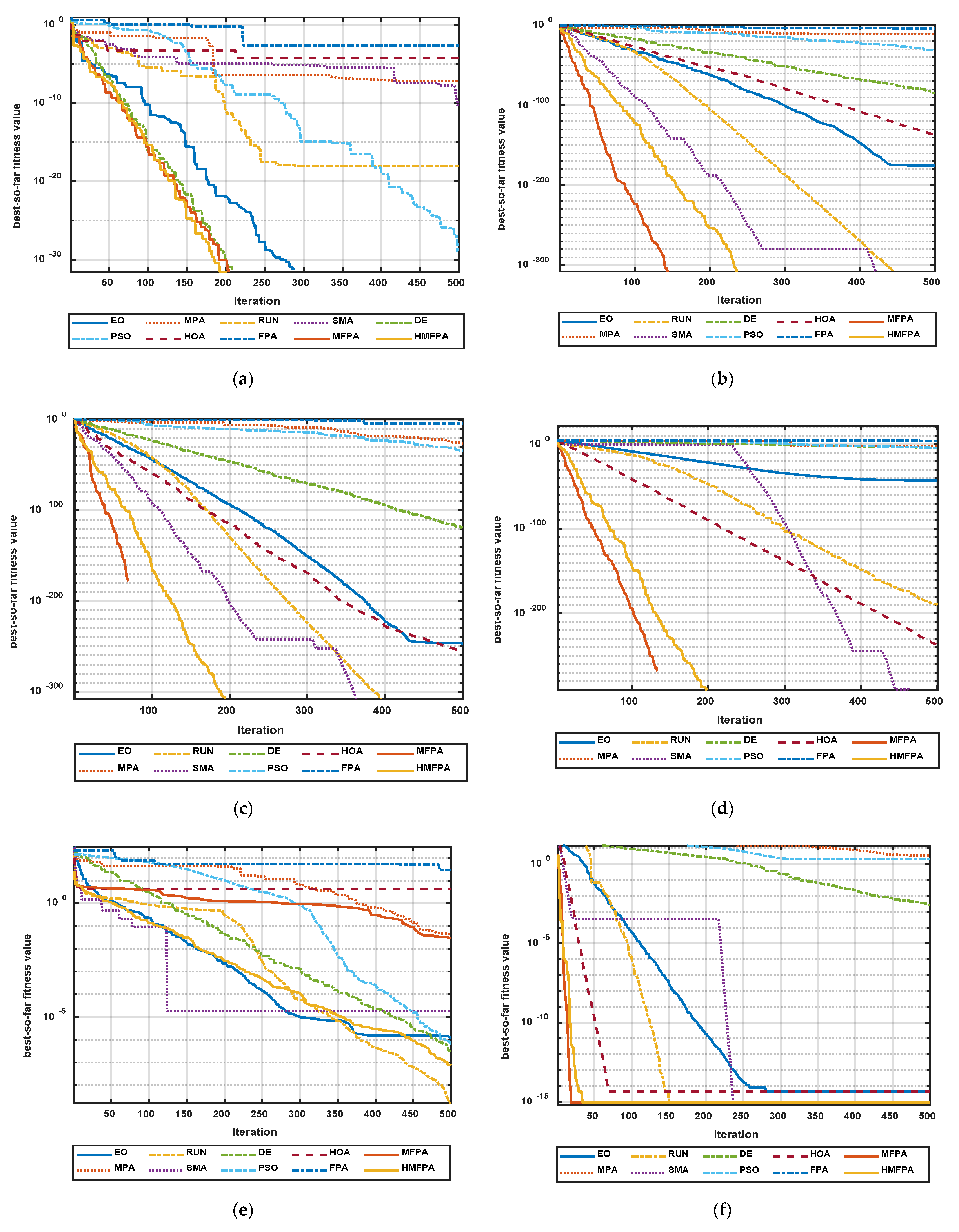
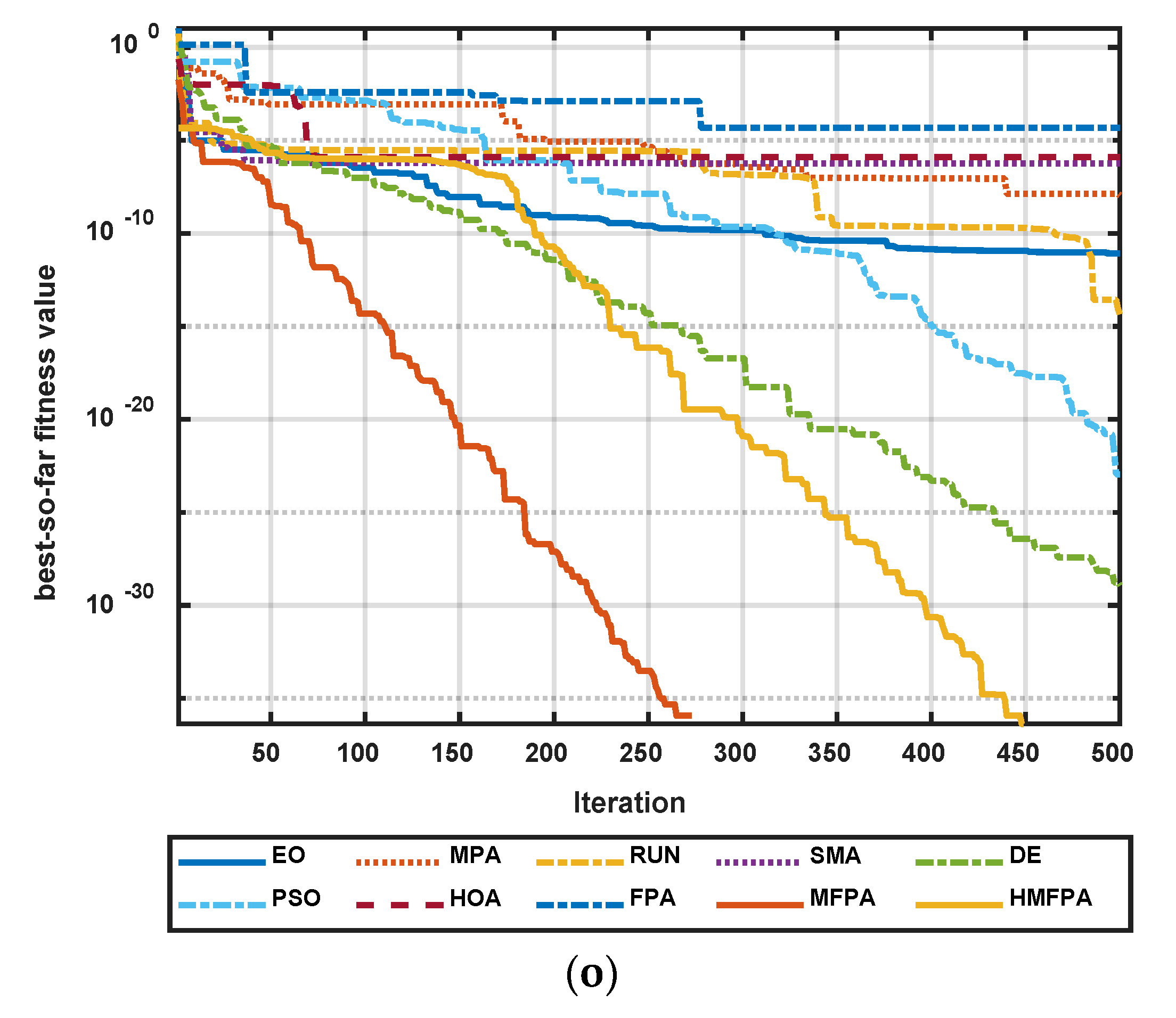
Furthermore, the convergence curve obtained by each algorithm in log scale is presented in Figure 7, on nine test functions randomly selected to show if any of them need fewer iterations to reach the optimal solution. This figure shows that MFPA could be superior for F2, F3, F6, F12, and F22, while both MFPA and HFPA were competitive with each other and superior to the other for the remainder, except F7, which has better convergence by RUN. This figure, which elaborates the superiority of the MFPA for most test functions, affirms that MFPA has a better exploitation operator than the HFPA, and this might not be effective for some optimization problems, which need higher exploration capabilities to cover the search space as possible for reaching the best solution.
Finally, to see if the speedup of our proposed algorithms is better or not, Figure 8 shows the average of the computational cost consumed by each algorithm on all test functions within the independent runs, which affirms that both HFPA and MFPA are almost competitive with PSO, and superior to the others, except for EO and FPA, which need less computational costs, but have worse performance in comparison to the proposed algorithms.
5.3. Comparison of the NESs
As a case study, the NESs are herein solved by the proposed algorithms: MFPA and HFPA, and their outcomes are compared with eight well-established optimization algorithms to see their superiority for tackling these equations. The proposed algorithms: MFPA and HFPA, in addition to the others, are executed 30 independent times and the analyzed outcomes are exhibited in Table 5 and Table 6, which show HFPA could have superior and equal performance for 18 out of 27 test functions with a percentage of 67%, as found in Figure 9, better than MFPA, which could be superior and competitive for only 10 NESs, with a success proportion of 37% as the second-best algorithm in all independent runs. For the other test functions, in the best case, HFPA could be competitive and superior to the competing algorithms for all employed NESs with a proportion of 100%, as found in Figure 9. This confirms the efficiency of integrating the DE with the MFPA, which gives this hybrid variant a higher influence for the exploration over the exploitation to preserve the population diversity, to prevent being stuck in local minima and, hence, reach better outcomes along the optimization process, as long as the population diversity is preserved.
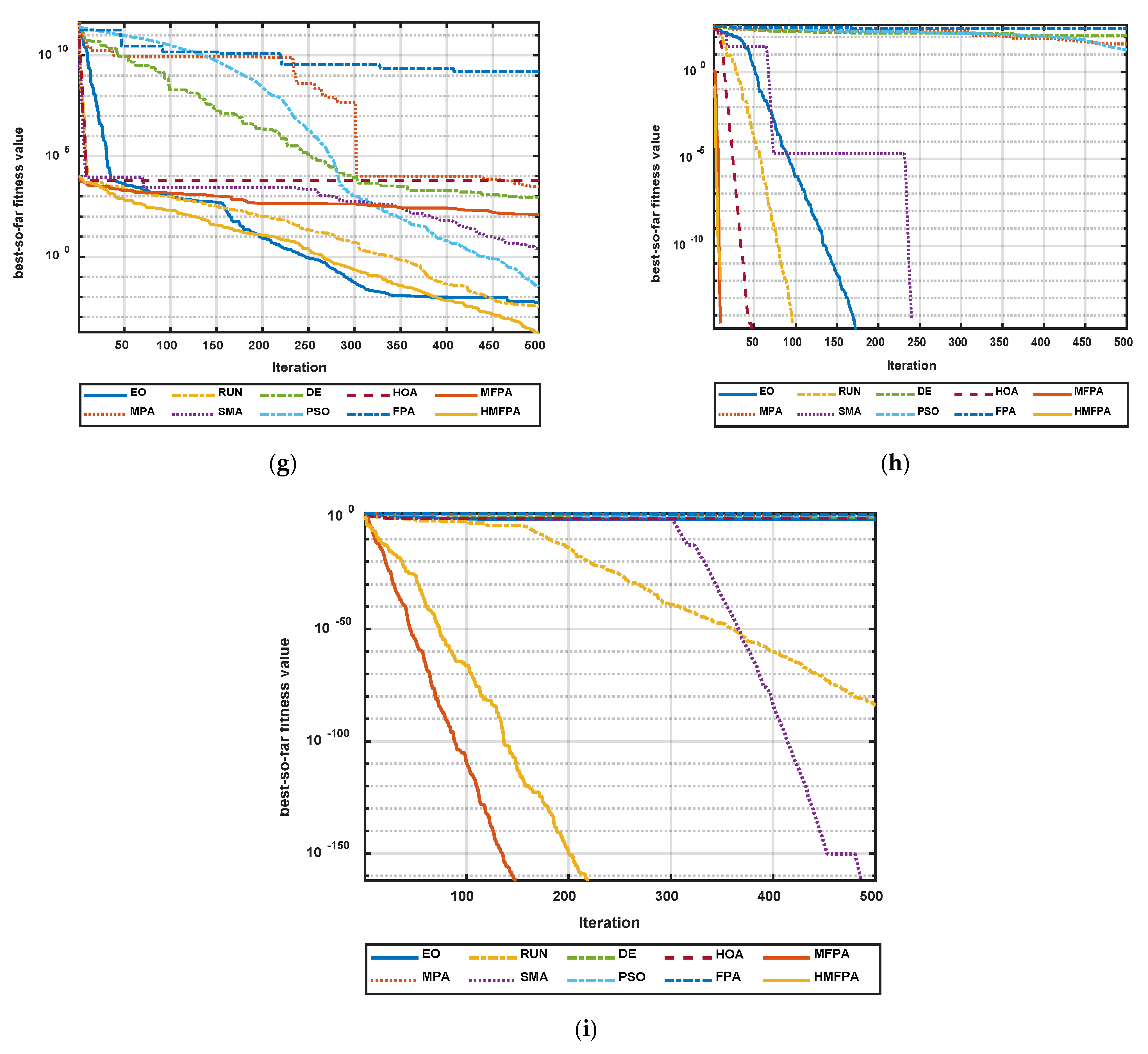
Furthermore, the convergence curves obtained by each algorithm in log scale are presented in Figure 10 to show if any of them needs fewer iterations to reach the optimal solution. This figure shows that MFPA could be superior for f1, f4, f13, f15, and f17; and HFPA for f2, f3, f7, f10, f11, and f12, while both are competitive with the others for the remaining functions depicted in Figure 10. Moreover, from Figure 10, it is noted that MFPA has better exploitation capability because it could reach the optimal solution using significantly smaller iterations than those needed by the other competing algorithms. MFPA for f3 has a worse convergence speed than most of the others because of weakening its exploration operator, which helps it keep the population diversity to explore several regions within the whole optimization process, in the hope of establishing the region, which has near-optimal solution. On the contrary, the HFPA on f3 could be superior to all the others in terms of the convergence speed, which notifies that HFPA balances between the exploration and exploitation capability to avoid being stuck in local minima, and accelerate the convergence speed to the near-optimal solution.
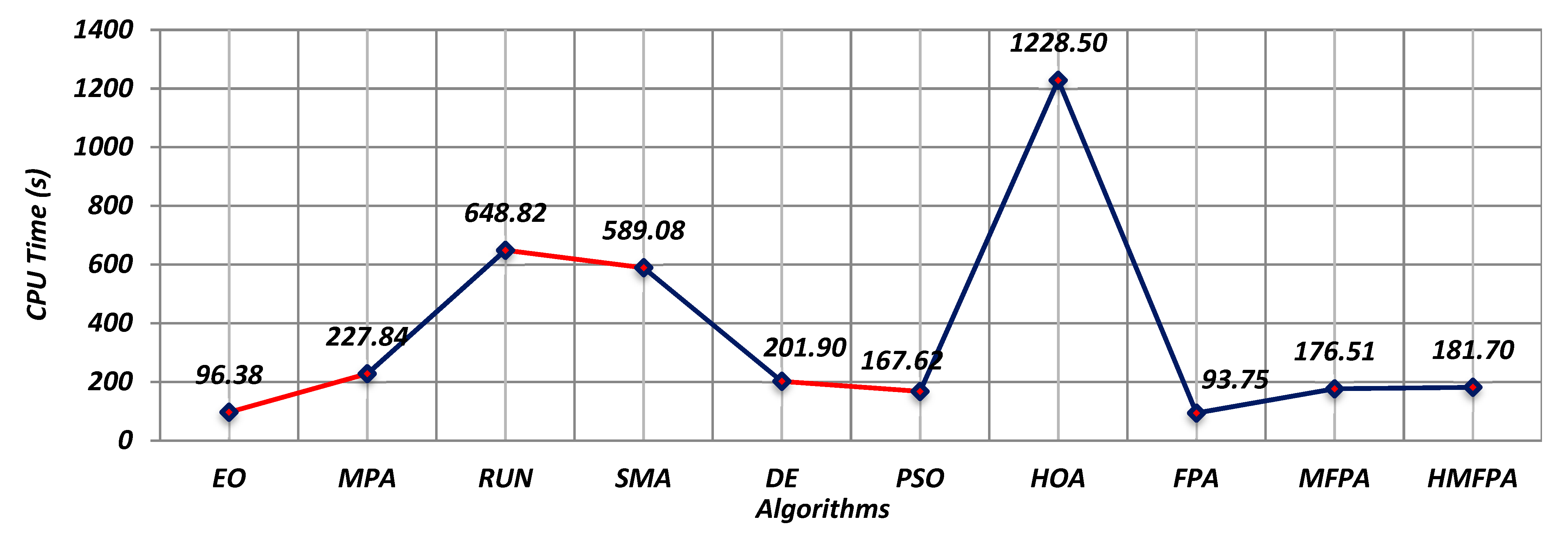
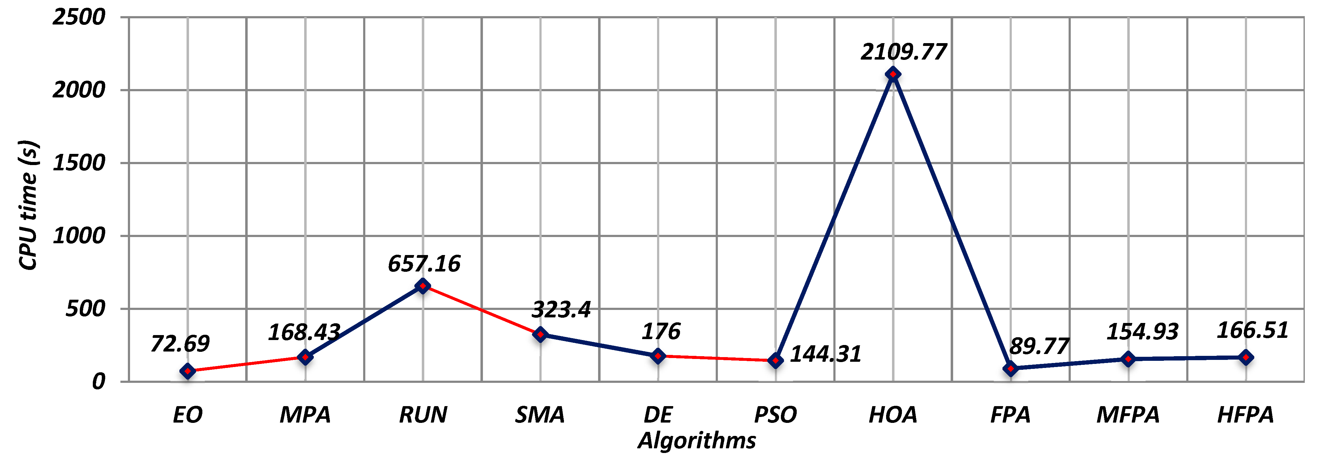
In addition, Figure 11 affirms that the average of the computational cost consumed by the proposed algorithm is superior to HOA, DE, MPA, RUN, and SMA; and competitive to PSO; however, unfortunately, they almost consume twice the time of both EO and FPA as our main future challenge.
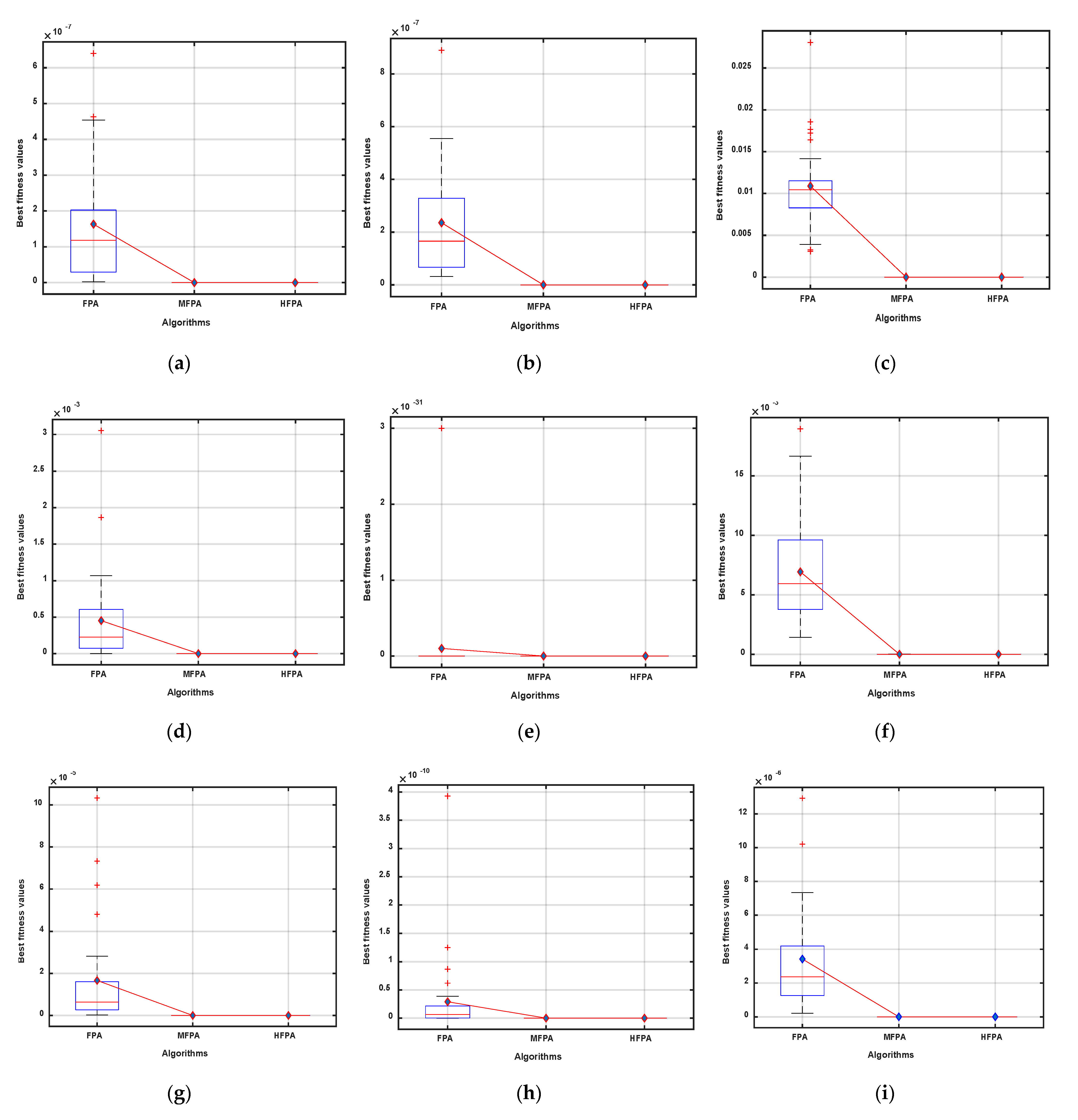
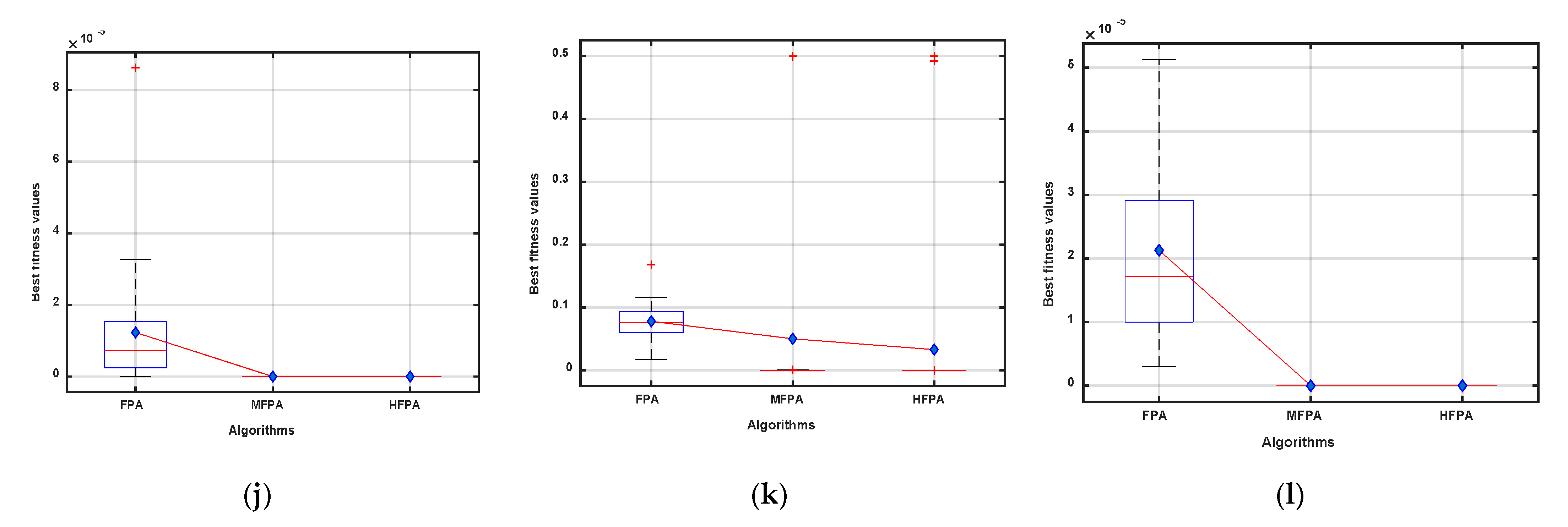
5.4. Comparison between FPA Variants on NESs
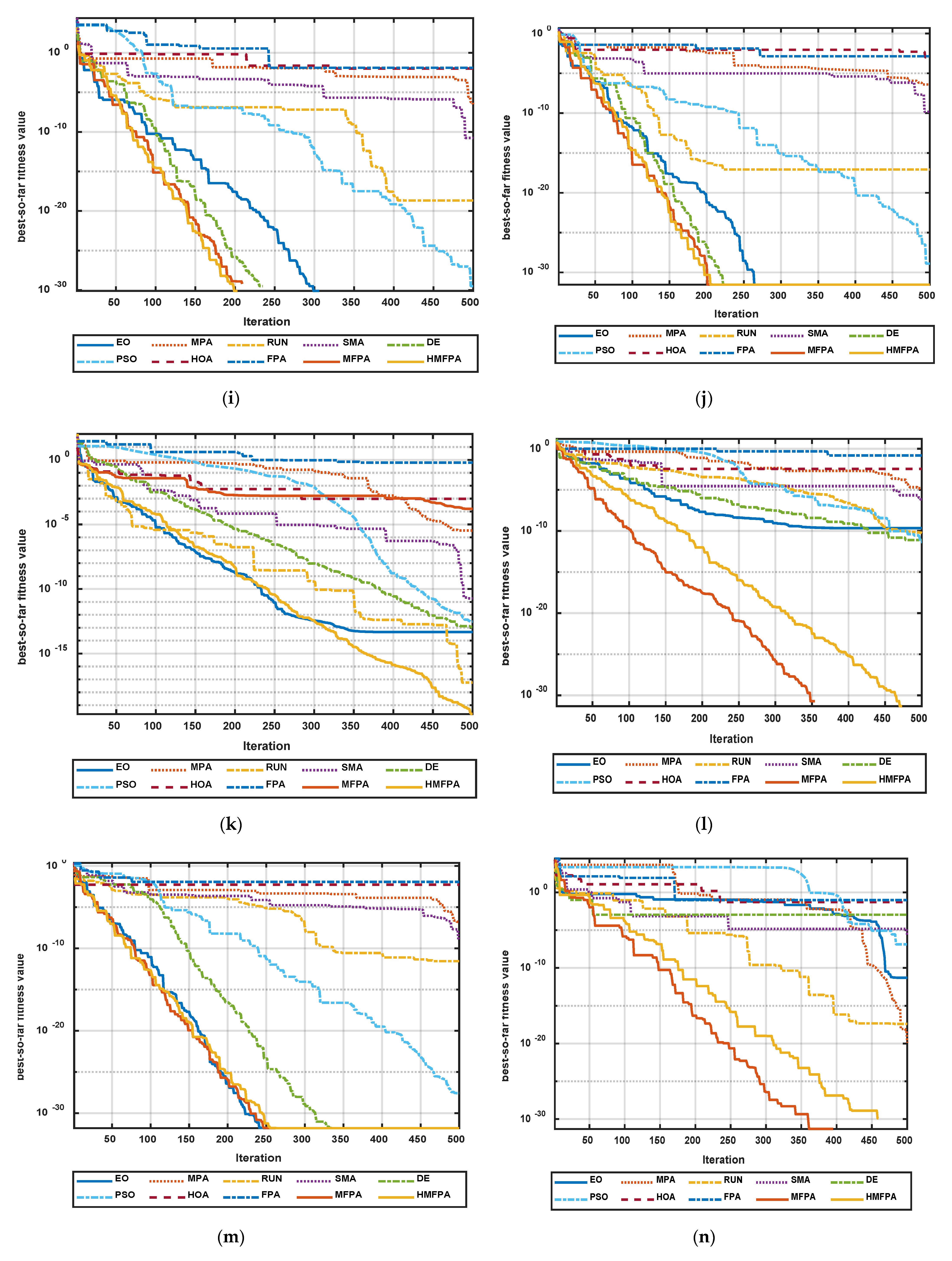
In this section, the proposed algorithms: HFPA and MFPA, in addition to the classical FPA, are compared with each other based on drawing the boxplot of the outcomes obtained by each various test function, and exposing the outcomes in Figure 12. From this figure, it is obvious that both MFPA and HFPA could be better than the classical FPA for all test functions, and both HFPA and MFPA have competitive performance.
6. Conclusions and Future Work
In this paper, the classical FPA is modified to improve its global pollination for exploring more regions in the search space to avoid being stuck in local minima. In addition, the local pollination is also modified to enhance the exploitation capability for searching extensively around the best-so-far solution to accelerate the convergence speed in the right direction of the near-optimal solution This modified variant is abbreviated MFPA. Furthermore, the differential evolution algorithm was integrated with this modified variant, effectively as an attempt to develop a new one, namely HFPA, having a high exploration operator. The proposed algorithms: MFPA and HFPA, and the classical FPA, in addition to seven well-known metaheuristic algorithms, were extensively assessed using 23 unimodal and multimodal mathematical test functions, and 27 widely used nonlinear equation systems. Their outcomes were statistically analyzed and compared with each other. The experimental findings affirm that both MFPA and HFPA are significantly competitive with each other and dramatically superior to the standard FPA. Moreover, these findings show that MFPA and HFPA are superior and competitive to the well-known compared metaheuristic algorithms in terms of final accuracy, computational cost, and convergence speed. Our future work involves proposing a binary variant of those two proposed algorithms for tackling the 0–1 knapsack, feature selection, and cryptanalysis of cipher-text, in addition to proposing another combinatorial algorithm to tackle the DNA fragment assembly problem. Moreover, in the future, we will search for a new strategy to balance between the exploration and exploitation operators of this modified variant to fulfill better outcomes.
Author Contributions
Conceptualization, M.A.-B., R.M., S.S.A. and M.A.; methodology, M.A.-B., R.M., S.S., M.A.; software, M.A-B., R.M., M.A.; validation, M.A.-B., S.S. and S.S.A.; formal analysis, M.A.-B., R.M. and M.A.; investigation, S.S.A., S.S. and M.A.; resources, M.A.-B., M.A. and R.M.; data curation, M.A.-B., S.S.A., R.M. and M.A.; writing—original draft preparation, M.A.-B., R.M. and M.A.; writing—review and editing, S.S.A., S.S. and M.A.; visualization, M.A.-B., M.A. and R.M.; supervision, M.A.-B., M.A. and S.S.A.; project administration, M.A.-B., S.S., R.M. and M.A.; funding acquisition, S.S.A. All authors have read and agreed to the published version of the manuscript.
Funding
This project is funded by King Saud University, Riyadh, Saudi Arabia.
Data Availability Statement
Not Applicable.
Acknowledgments
Research Supporting Project number (RSP-2021/167), King Saud University, Riyadh, Saudi Arabia.
Conflicts of Interest
The authors declare no conflict of interest.
References
- Mirjalili, S.; Lewis, A. The Whale Optimization Algorithm. Adv. Eng. Softw. 2016, 95, 51–67. [Google Scholar] [CrossRef]
- Holland, J.H. Genetic Algorithms. Sci. Am. 1992, 267, 66–73. [Google Scholar] [CrossRef]
- Rechenberg, I. Evolutionsstrategien, in Simulationsmethoden in der Medizin und Biologie; Springer: Berlin/Heidelberg, Germany, 1978; pp. 83–114. [Google Scholar]
- Banzhaf, W.; Nordin, P.; Keller, R.E.; Francone, F.D. Genetic Programming: An Introduction; Morgan Kaufmann Publishers: San Francisco, CA, USA, 1998; Volume 1. [Google Scholar]
- Dasgupta, D.; Michalewicz, Z. Evolutionary Algorithms in Engineering Applications; Springer Science & Business Media: Berlin/Heidelberg, Germany, 2013. [Google Scholar]
- Simon, D. Biogeography-Based Optimization. IEEE Trans. Evol. Comput. 2008, 12, 702–713. [Google Scholar] [CrossRef] [Green Version]
- Van Laarhoven, P.J.M.; Aarts, E.H.L. Simulated Annealing: Theory and Applications; Springer Science and Business Media LLC: Berlin/Heidelberg, Germany, 1987; pp. 7–15. [Google Scholar]
- Erol, O.K.; Eksin, I. A New Optimization Method: Big Bang–Big Crunch. Adv. Eng. Softw. 2006, 37, 106–111. [Google Scholar] [CrossRef]
- Rashedi, E.; Nezamabadi-Pour, H.; Saryazdi, S. GSA: A Gravitational Search Algorithm. Inf. Sci. 2009, 179, 2232–2248. [Google Scholar] [CrossRef]
- Du, H.; Wu, X.; Zhuang, J. Small-World Optimization Algorithm for Function Optimization. In Proceedings of the Transactions on Petri Nets and Other Models of Concurrency XV; Springer Science and Business Media LLC: Berlin/Heidelberg, Germany, 2006; pp. 264–273. [Google Scholar]
- Moghaddam, F.F.; Moghaddam, R.F.; Cheriet, M. Curved Space Optimization: A Random Search Based on General Relativity Theory. arXiv 2012, arXiv:1208.2214. [Google Scholar]
- Hosseini, H.S. Principal Components Analysis by the Galaxy-Based Search Algorithm: A Novel Metaheuristic for Continuous Optimisation. Int. J. Comput. Sci. Eng. 2011, 6, 132. [Google Scholar] [CrossRef]
- Kaveh, A.; Talatahari, S. A Novel Heuristic Optimization Method: Charged System Search. Acta Mech. 2010, 213, 267–289. [Google Scholar] [CrossRef]
- Van Tran, T.; Wang, Y. Informatics, Artificial Chemical Reaction Optimization Algorithm and Neural Network Based Adaptive Control for Robot Manipulator. J. Control. Eng. Appl. Inform. 2017, 19, 61–70. [Google Scholar]
- Kaveh, A.; Khayatazad, M. A New Meta-Heuristic Method: Ray Optimization. Comput. Struct. 2012, 112-113, 283–294. [Google Scholar] [CrossRef]
- Faramarzi, A.; Heidarinejad, M.; Stephens, B.; Mirjalili, S. Equilibrium Optimizer: A Novel Optimization Algorithm. Knowl. Based Syst. 2020, 191, 105190. [Google Scholar] [CrossRef]
- Kaveh, A.; Khanzadi, M.; Moghaddam, M.R. Billiards-Inspired Optimization Algorithm; A New Meta-Heuristic Method. Structures 2020, 27, 1722–1739. [Google Scholar] [CrossRef]
- Hatamlou, A. Black Hole: A New Heuristic Optimization Approach for Data Clustering. Inf. Sci. 2013, 222, 175–184. [Google Scholar] [CrossRef]
- Kennedy, J.; Eberhart, R. Particle Swarm Optimization. In Proceedings of the ICNN’95 International Conference on Neural Networks, Perth, Australia, 27 November–1 December 1995; Volume 4, pp. 1942–1948. [Google Scholar]
- Heidari, A.A.; Mirjalili, S.; Faris, H.; Aljarah, I.; Mafarja, M.; Chen, H. Harris Hawks Optimization: Algorithm and Applications. Futur. Gener. Comput. Syst. 2019, 97, 849–872. [Google Scholar] [CrossRef]
- Faramarzi, A.; Heidarinejad, M.; Mirjalili, S.; Gandomi, A.H. Marine Predators Algorithm: A Nature-Inspired Metaheuristic. Expert Syst. Appl. 2020, 152, 113377. [Google Scholar] [CrossRef]
- Li, S.; Chen, H.; Wang, M.; Heidari, A.A.; Mirjalili, S. Slime Mould Algorithm: A New Method for Stochastic Optimization. Future Gener. Comput. Syst. 2020, 111, 300–323. [Google Scholar] [CrossRef]
- Dorigo, M.; Birattari, M.; Stutzle, T. Ant Colony Optimization. IEEE Comput. Intell. Mag. 2006, 1, 28–39. [Google Scholar] [CrossRef] [Green Version]
- Mirjalili, S.; Mirjalili, S.M.; Lewis, A. Grey Wolf Optimizer. Adv. Eng. Softw. 2014, 69, 46–61. [Google Scholar] [CrossRef] [Green Version]
- Gandomi, A.H.; Yang, X.-S.; Alavi, A.H. Erratum to: Cuckoo Search Algorithm: A Metaheuristic Approach to Solve Structural Optimization Problems. Eng. Comput. 2013, 29, 245. [Google Scholar] [CrossRef] [Green Version]
- Yang, X.-S.; He, X. Bat Algorithm: Literature Review and Applications. Int. J. Bio-Inspired Comput. 2013, 5, 141–149. [Google Scholar] [CrossRef] [Green Version]
- Yang, X.-S. Flower Pollination Algorithm for Global Optimization. In Proceedings of the Transactions on Petri Nets and Other Models of Concurrency XV; Springer Science and Business Media LLC: Berlin/Heidelberg, Germany, 2012; pp. 240–249. [Google Scholar]
- Khishe, M.; Mosavi, M. Chimp Optimization Algorithm. Expert Syst. Appl. 2020, 149, 113338. [Google Scholar] [CrossRef]
- Chu, S.-C.; Tsai, P.-W.; Pan, J.-S. Cat Swarm Optimization. In Proceedings of the 9th Pacific Rim International Conference on Artificial Intelligence, Guilin, China, 7–11 August 2006. [Google Scholar]
- Meng, X.-B.; Liu, Y.; Gao, X.; Zhang, H. A New Bio-inspired Algorithm: Chicken Swarm Optimization. In Proceedings of the 5th International Conference (ICSI 2014), Hefei, China, 17–20 October 2014; pp. 86–94. [Google Scholar]
- Bansal, J.C.; Sharma, H.; Jadon, S.S.; Clerc, M. Spider Monkey Optimization Algorithm for Numerical Optimization. Memetic Comput. 2014, 6, 31–47. [Google Scholar] [CrossRef]
- Gandomi, A.H.; Alavi, A.H. Krill Herd: A New Bio-Inspired Optimization Algorithm. Commun. Nonlinear Sci. Numer. Simul. 2012, 17, 4831–4845. [Google Scholar] [CrossRef]
- Xing, B.; Gao, W.-J. Innovative Computational Intelligence: A Rough Guide to 134 Clever Algorithms; Springer Science and Business Media LLC: Berlin/Heidelberg, Germany, 2014; pp. 167–170. [Google Scholar]
- Kaveh, A.; Farhoudi, N. A New Optimization Method: Dolphin Echolocation. Adv. Eng. Softw. 2013, 59, 53–70. [Google Scholar] [CrossRef]
- Oftadeh, R.; Mahjoob, M.; Shariatpanahi, M. A Novel Meta-Heuristic Optimization Algorithm Inspired by Group Hunting of Animals: Hunting Search. Comput. Math. Appl. 2010, 60, 2087–2098. [Google Scholar] [CrossRef] [Green Version]
- Yang, X.-S. Firefly Algorithms for Multimodal Optimization. In International Symposium on Stochastic Algorithms; Springer: Berlin/Heidelberg, Germany, 2009; pp. 169–178. [Google Scholar]
- Shiqin, Y.; Jianjun, J.; Guangxing, Y. A Dolphin Partner Optimization. In Proceedings of the 2009 WRI Global Congress on Intelligent Systems, Xiamen, China, 19–21 May 2009; Volume 1, pp. 124–128. [Google Scholar] [CrossRef]
- Lu, X.; Zhou, Y. A Novel Global Convergence Algorithm: Bee Collecting Pollen Algorithm. In Proceedings of the 4th International Conference on Intelligent Computing, ICIC 2008, Shanghai, China, 15–18 September 2008; pp. 518–525. [Google Scholar]
- Wu, H.; Zhang, F.-M. Wolf Pack Algorithm for Unconstrained Global Optimization. Math. Probl. Eng. 2014, 2014, 465082. [Google Scholar] [CrossRef] [Green Version]
- Pilat, M.L. Wasp-Inspired Construction Algorithms; University of Calgary: Calgary, AB, Canda, 2006. [Google Scholar]
- Rao, R.V. Teaching-Learning-Based Optimization Algorithm. In Teaching Learning Based Optimization Algorithm; Springer: Berlin/Heidelberg, Germany, 2016; pp. 9–39. [Google Scholar]
- Geem, Z.W.; Kim, J.H.; Loganathan, G. A New Heuristic Optimization Algorithm: Harmony Search. Simulation 2001, 76, 60–68. [Google Scholar] [CrossRef]
- Kashan, A.H. League Championship Algorithm: A New Algorithm for Numerical Function Optimization. In Proceedings of the 2009 International Conference of Soft Computing and Pattern Recognition, Malacca, Malaysia, 4–7 December 2009; pp. 43–48. [Google Scholar]
- Eita, M.; Fahmy, M. Group Counseling Optimization. Appl. Soft Comput. 2014, 22, 585–604. [Google Scholar] [CrossRef]
- Eita, M.A.; Fahmy, M.M. Group Counseling Optimization: A Novel Approach. In Research and Development in Intelligent Systems XXVI; Springer Science and Business Media LLC: Berlin/Heidelberg, Germany, 2009; pp. 195–208. [Google Scholar]
- Sadollah, A.; Bahreininejad, A.; Eskandar, H.; Hamdi, M. Mine Blast Algorithm: A New Population Based Algorithm for Solving Constrained Engineering Optimization Problems. Appl. Soft Comput. 2013, 13, 2592–2612. [Google Scholar] [CrossRef]
- Dai, C.; Zhu, Y.; Chen, W. Seeker Optimization Algorithm. In International Conference on Computational and Information Science; Springer: Berlin/Heidelberg, Germany, 2006. [Google Scholar]
- Moosavian, N.; Roodsari, B.K.J. Soccer League Competition Algorithm, A New Method for Solving Systems of Nonlinear Equations. Int. J. Intell. Sci. 2013, 4, 7. [Google Scholar] [CrossRef]
- Moosavian, N.; Roodsari, B.K. Soccer League Competition Algorithm: A Novel Meta-Heuristic Algorithm for Optimal Design of Water Distribution Networks. Swarm Evol. Comput. 2014, 17, 14–24. [Google Scholar] [CrossRef]
- Tan, Y.; Zhu, Y. Fireworks Algorithm for Optimization. In Proceedings of the Transactions on Petri Nets and Other Models of Concurrency XV; Springer Science and Business Media LLC: Berlin/Heidelberg, Germany, 2010; pp. 355–364. [Google Scholar]
- Moosavi, S.H.S.; Bardsiri, V.K. Poor and Rich Optimization Algorithm: A New Human-Based and Multi Populations Algorithm. Eng. Appl. Artif. Intell. 2019, 86, 165–181. [Google Scholar] [CrossRef]
- Liao, Z.; Gong, W.; Wang, L. Memetic Niching-Based Evolutionary Algorithms for Solving Nonlinear Equation System. Expert Syst. Appl. 2020, 149, 113261. [Google Scholar] [CrossRef]
- Wetweerapong, J.; Puphasuk, P. An Improved Differential Evolution Algorithm with a Restart Technique to Solve Systems of Nonlinear Equations. Int. J. Optim. Control. Theor. Appl. 2020, 10, 118–136. [Google Scholar] [CrossRef] [Green Version]
- Boussaïd, I.; Lepagnot, J.; Siarry, P. A Survey on Optimization Metaheuristics. Inf. Sci. 2013, 237, 82–117. [Google Scholar] [CrossRef]
- Siddique, N.H.; Adeli, H. Nature Inspired Computing: An Overview and Some Future Directions. Cogn. Comput. 2015, 7, 706–714. [Google Scholar] [CrossRef] [PubMed] [Green Version]
- Nabil, E. A Modified Flower Pollination Algorithm for Global Optimization. Expert Syst. Appl. 2016, 57, 192–203. [Google Scholar] [CrossRef]
- Yang, X.-S.; Karamanoglu, M.; He, X. Flower Pollination Algorithm: A Novel Approach for Multiobjective Optimization. Eng. Optim. 2014, 46, 1222–1237. [Google Scholar] [CrossRef] [Green Version]
- Nigdeli, S.M.; Bekdaş, G.; Yang, X.-S. Application of the Flower Pollination Algorithm in Structural Engineering. In Internet of Things (IoT) in 5G Mobile Technologies; Springer Science and Business Media LLC: Berlin/Heidelberg, Germany, 2016; pp. 25–42. [Google Scholar]
- Rodrigues, D.; Yang, X.-S.; de Souza, A.N.; Papa, J.P. Binary Flower Pollination Algorithm and Its Application to Feature Selection. In Econometrics for Financial Applications; Springer Science and Business Media LLC: Berlin/Heidelberg, Germany, 2015; pp. 85–100. [Google Scholar]
- Salgotra, R.; Singh, U. Application of Mutation Operators to Flower Pollination Algorithm. Expert Syst. Appl. 2017, 79, 112–129. [Google Scholar] [CrossRef]
- Wang, R.; Zhou, Y.; Qiao, S.; Huang, K. Flower Pollination Algorithm with Bee Pollinator for Cluster Analysis. Inf. Process. Lett. 2016, 116, 1–14. [Google Scholar] [CrossRef] [Green Version]
- Storn, R. On the Usage of Differential Evolution for Function Optimization. In Proceedings of the North American Fuzzy Information Processing, Berkeley, CA, USA, 19–22 June 1996; pp. 519–523. [Google Scholar] [CrossRef]
- Mohamed, A.W.; Sabry, H.Z.; Khorshid, M. An Alternative Differential Evolution Algorithm for Global Optimization. J. Adv. Res. 2012, 3, 149–165. [Google Scholar] [CrossRef] [Green Version]
- Karaboğa, D.; Ökdem, S.J.; Sciences, C. A Simple and Global Optimization Algorithm for Engineering Problems: Differential Evolution Algorithm. Turk. J. Electr. Eng. Comput. Sci. 2004, 12, 53–60. [Google Scholar]
- Das, S.; Mandal, A.; Mukherjee, R. An Adaptive Differential Evolution Algorithm for Global Optimization in Dynamic Environments. IEEE Trans. Cybern. 2013, 44, 966–978. [Google Scholar] [CrossRef]
- Huang, Z.; Wang, C.-E.; Ma, M. A Robust Archived Differential Evolution Algorithm for Global Optimization Problems. J. Comput. 2009, 4, 160–167. [Google Scholar] [CrossRef]
- Pant, M.; Ali, M.; Singh, V.P. Parent-Centric Differential Evolution Algorithm for Global Optimization Problems. Opsearch 2009, 46, 153–168. [Google Scholar] [CrossRef]
- Choi, T.J.; Ahn, C.W.; An, J. An Adaptive Cauchy Differential Evolution Algorithm for Global Numerical Optimization. Sci. World J. 2013, 2013, 969734. [Google Scholar] [CrossRef] [PubMed] [Green Version]
- Kumar, P.; Pant, M. A Self Adaptive Differential Evolution Algorithm for Global Optimization. In Proceedings of the Computer Vision; Springer Science and Business Media LLC: Berlin/Heidelberg, Germany, 2010; Volume 6466, pp. 103–110. [Google Scholar]
- Sun, J.; Zhang, Q.; Tsang, E.P.K. DE/EDA: A New Evolutionary Algorithm for Global Optimization. Inf. Sci. 2005, 169, 249–262. [Google Scholar] [CrossRef]
- Brest, J.; Zamuda, A.; Fister, I.; Maucec, M.S. Large Scale Global Optimization Using Self-Adaptive Differential Evolution Algorithm. In Proceedings of the IEEE Congress on Evolutionary Computation, Barcelona, Spain, 18–23 July 2010; pp. 1–8. [Google Scholar]
- Yi, W.; Gao, L.; Li, X.; Zhou, Y. A New Differential Evolution Algorithm with a Hybrid Mutation Operator and Self-Adapting Control Parameters for Global Optimization Problems. Appl. Intell. 2014, 42, 642–660. [Google Scholar] [CrossRef]
- Brest, J.; Zumer, V.; Maucec, M. Self-Adaptive Differential Evolution Algorithm in Constrained Real-Parameter Optimization. In Proceedings of the 2006 IEEE International Conference on Evolutionary Computation, Vancouver, BC, Canada, 16–21 July 2006. [Google Scholar]
- Ramadas, G.C.; Fernandes, E.M.d.G. Solving Systems of Nonlinear Equations by Harmony Search. In Proceedings of the 13th International Conference on Mathematical Methods in Science and Engineering, Almeria, Spain, 24–27 June 2013. [Google Scholar]
- Wu, J.; Cui, Z.; Liu, J. Using Hybrid Social Emotional Optimization Algorithm with Metropolis Rule to Solve Nonlinear Equations. In Proceedings of the IEEE 10th International Conference on Cognitive Informatics and Cognitive Computing (ICCI-CC’11), Banff, AB, Canada, 18–20 August 2011; pp. 405–411. [Google Scholar]
- Chang, W.-D. An Improved Real-Coded Genetic Algorithm for Parameters Estimation of Nonlinear Systems. Mech. Syst. Signal. Process. 2006, 20, 236–246. [Google Scholar] [CrossRef]
- Grosan, C.; Abraham, A. A New Approach for Solving Nonlinear Equations Systems. IEEE Trans. Syst. Man Cybern. Part A Syst. Hum. 2008, 38, 698–714. [Google Scholar] [CrossRef]
- Ren, H.; Wu, L.; Bi, W.; Argyros, I.K. Solving Nonlinear Equations System via an Efficient Genetic Algorithm with Symmetric and Harmonious Individuals. Appl. Math. Comput. 2013, 219, 10967–10973. [Google Scholar] [CrossRef]
- Mo, Y.; Liu, H.; Wang, Q. Conjugate Direction Particle Swarm Optimization Solving Systems of Nonlinear Equations. Comput. Math. Appl. 2009, 57, 1877–1882. [Google Scholar] [CrossRef] [Green Version]
- Jaberipour, M.; Khorram, E.; Karimi, B. Particle Swarm Algorithm for Solving Systems of Nonlinear Equations. Comput. Math. Appl. 2011, 62, 566–576. [Google Scholar] [CrossRef] [Green Version]
- Ariyaratne, M.; Fernando, T.; Weerakoon, S. Solving Systems of Nonlinear Equations Using a Modified Firefly Algorithm (MODFA). Swarm Evol. Comput. 2019, 48, 72–92. [Google Scholar] [CrossRef]
- Wu, Z.; Kang, L. A Fast and Elitist Parallel Evolutionary Algorithm for Solving Systems of Non-Linear Equations. In Proceedings of the 2003 Congress on Evolutionary Computation, CEC ’03, Canberra, Australia, 8–12 December 2003. [Google Scholar]
- El-Shorbagy, M.A.; El-Refaey, A.M. Hybridization of Grasshopper Optimization Algorithm With Genetic Algorithm for Solving System of Non-Linear Equations. IEEE Access 2020, 8, 220944–220961. [Google Scholar] [CrossRef]
- Ibrahim, A.M.; Tawhid, M.A. A Hybridization of Differential Evolution and Monarch Butterfly Optimization for Solving Systems of Nonlinear Equations. J. Comput. Des. Eng. 2018, 6, 354–367. [Google Scholar] [CrossRef]
- Pant, S.; Kumar, A.; Ram, M. Solution of Nonlinear Systems of Equations via Metaheuristics. Int. J. Math. Eng. Manag. Sci. 2019, 4, 1108–1126. [Google Scholar] [CrossRef]
- Ibrahim, A.M.; Tawhid, M.A. Conjugate Direction DE Algorithm for Solving Systems of Nonlinear Equations. Appl. Math. Inf. Sci. 2017, 11, 339–352. [Google Scholar] [CrossRef]
- Zhang, X.; Wan, Q.; Fan, Y. Applying Modified Cuckoo Search Algorithm for Solving Systems of Nonlinear Equations. Neural Comput. Appl. 2017, 31, 553–576. [Google Scholar] [CrossRef]
- Ibrahim, A.M.; Tawhid, M.A. A Hybridization of Cuckoo Search and Particle Swarm Optimization for Solving Nonlinear Systems. Evol. Intell. 2019, 12, 541–561. [Google Scholar] [CrossRef]
- Xie, J.; Zhou, Y.; Chen, H. A Novel Bat Algorithm Based on Differential Operator and Lévy Flights Trajectory. Comput. Intell. Neurosci. 2013, 2013, 1–13. [Google Scholar] [CrossRef] [PubMed] [Green Version]
- Hassan, O.F.; Jamal, A.; Abdel-Khalek, S. Genetic Algorithm and Numerical Methods for Solving Linear and Nonlinear System of Equations: A Comparative Study. J. Intell. Fuzzy Syst. 2020, 38, 2867–2872. [Google Scholar] [CrossRef]
- Tawhid, M.A.; Ibrahim, A.M. A Hybridization of Grey Wolf Optimizer and Differential Evolution for Solving Nonlinear Systems. Evol. Syst. 2019, 11, 65–87. [Google Scholar] [CrossRef]
- Luo, Y.-Z.; Tang, G.-J.; Zhou, L.-N. Hybrid Approach for Solving Systems of Nonlinear Equations Using Chaos Optimization and Quasi-Newton Method. Appl. Soft Comput. 2008, 8, 1068–1073. [Google Scholar] [CrossRef]
- Wu, J.; Gong, W.; Wang, L. A Clustering-Based Differential Evolution with Different Crowding Factors for Nonlinear Equations system. Appl. Soft Comput. 2021, 98, 106733. [Google Scholar] [CrossRef]
- Mangla, C.; Ahmad, M.; Uddin, M. Optimization of Complex Nonlinear Systems Using Genetic Algorithm. Int. J. Inf. Technol. 2020. [Google Scholar] [CrossRef]
- Pourjafari, E.; Mojallali, H. Solving Nonlinear Equations Systems with a New Approach Based on Invasive Weed Optimization Algorithm and Clustering. Swarm Evol. Comput. 2012, 4, 33–43. [Google Scholar] [CrossRef]
- Storn, R. Differrential Evolution-A Simple and Efficient Adaptive Scheme for Global Optimization over Continuous Spaces; Technical report; International Computer Science Institute: Berkeley, CA, USA, 1995; p. 11. [Google Scholar]
- MiarNaeimi, F.; Azizyan, G.; Rashki, M. Horse Herd Optimization Algorithm: A Nature-Inspired Algorithm for High-Dimensional Optimization Problems. Knowl. Based Syst. 2021, 213, 106711. [Google Scholar] [CrossRef]
- Ahmadianfar, I.; Heidari, A.A.; Gandomi, A.H.; Chu, X.; Chen, H. RUN Beyond the Metaphor: An Efficient Optimization Algorithm Based on Runge Kutta Method. Expert Syst. Appl. 2021, 181, 115079. [Google Scholar] [CrossRef]
- Brest, J.; Maučec, M.S. Population Size Reduction for the Differential Evolution Algorithm. Appl. Intell. 2007, 29, 228–247. [Google Scholar] [CrossRef]
- Song, W.; Wang, Y.; Li, H.-X.; Cai, Z. Locating Multiple Optimal Solutions of Nonlinear Equation Systems Based on Multiobjective Optimization. IEEE Trans. Evol. Comput. 2015, 19, 414–431. [Google Scholar] [CrossRef]
- Sacco, W.; Henderson, N. Finding All Solutions of Nonlinear Systems Using a Hybrid Metaheuristic with Fuzzy Clustering Means. Appl. Soft Comput. 2011, 11, 5424–5432. [Google Scholar] [CrossRef]
- Hirsch, M.J.; Pardalos, P.M.; Resende, M.G. Solving Systems of Nonlinear Equations with Continuous GRASP. Nonlinear Anal. Real World Appl. 2009, 10, 2000–2006. [Google Scholar] [CrossRef]
- Sharma, J.R.; Arora, H. On Efficient Weighted-Newton Methods for Solving Systems of Nonlinear Equations. Appl. Math. Comput. 2013, 222, 497–506. [Google Scholar] [CrossRef]
- Junior, H.A.E.O.; Ingber, L.; Petraglia, A.; Petraglia, M.R.; Machado, M.A.S. Stochastic Global Optimization and Its Applications with Fuzzy Adaptive Simulated Annealing; Springer Science and Business Media LLC: Berlin/Heidelberg, Germany, 2012; pp. 33–62. [Google Scholar]
- Morgan, A.; Shapiro, V. Box-Bisection for Solving Second-Degree Systems and the Problem of Clustering. ACM Trans. Math. Softw. 1987, 13, 152–167. [Google Scholar] [CrossRef]
- Grau-Sánchez, M.; Grau, À.; Noguera, M. Frozen Divided Difference Scheme for Solving Systems of Nonlinear Equations. J. Comput. Appl. Math. 2011, 235, 1739–1743. [Google Scholar] [CrossRef]
- Waziri, M.; Leong, W.J.; Hassan, M.A.; Monsiet, M. An Efficient Solver for Systems of Nonlinear Equations with Singular Jacobian via Diagonal Updating. Appl. Math. Sci. 2010, 4, 3403–3412. [Google Scholar]
Figure 1.
Flowchart of the paper organization.
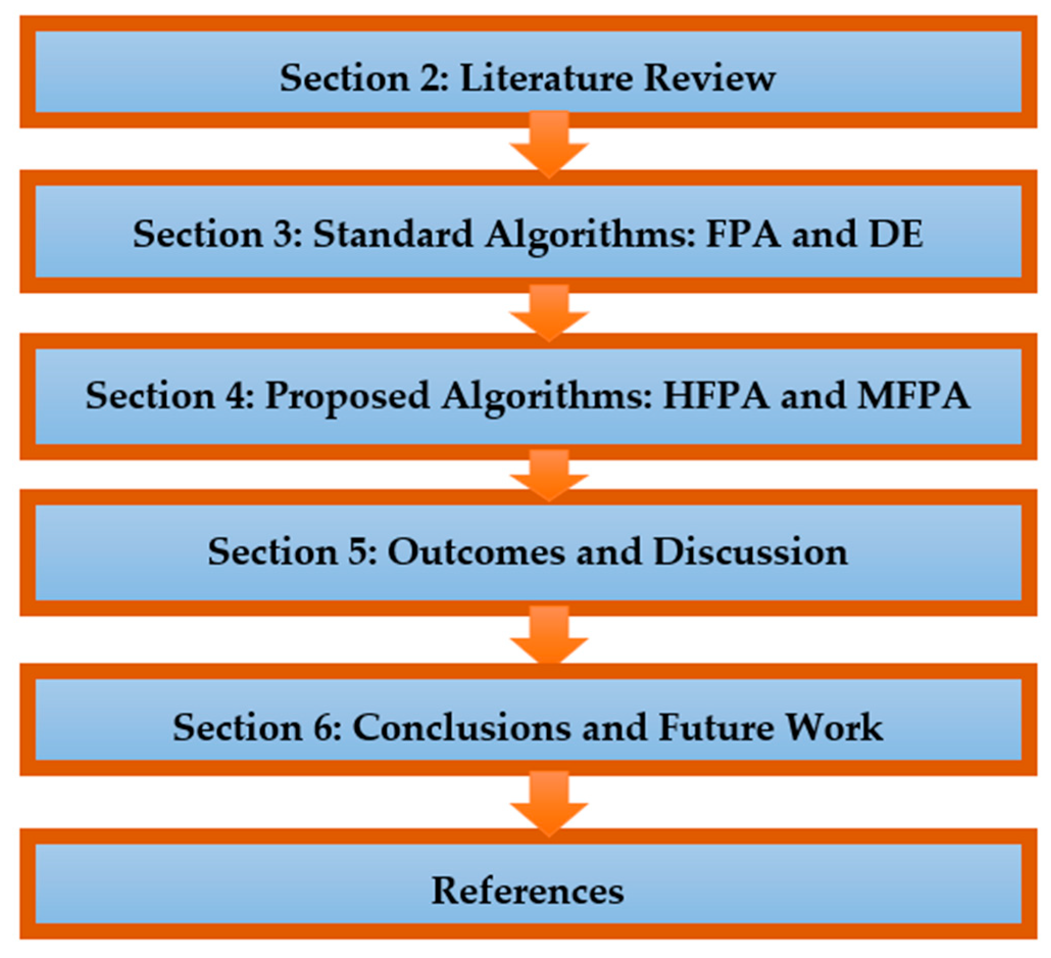
Figure 2.
Flowchart of MFPA for tackling the NESs.
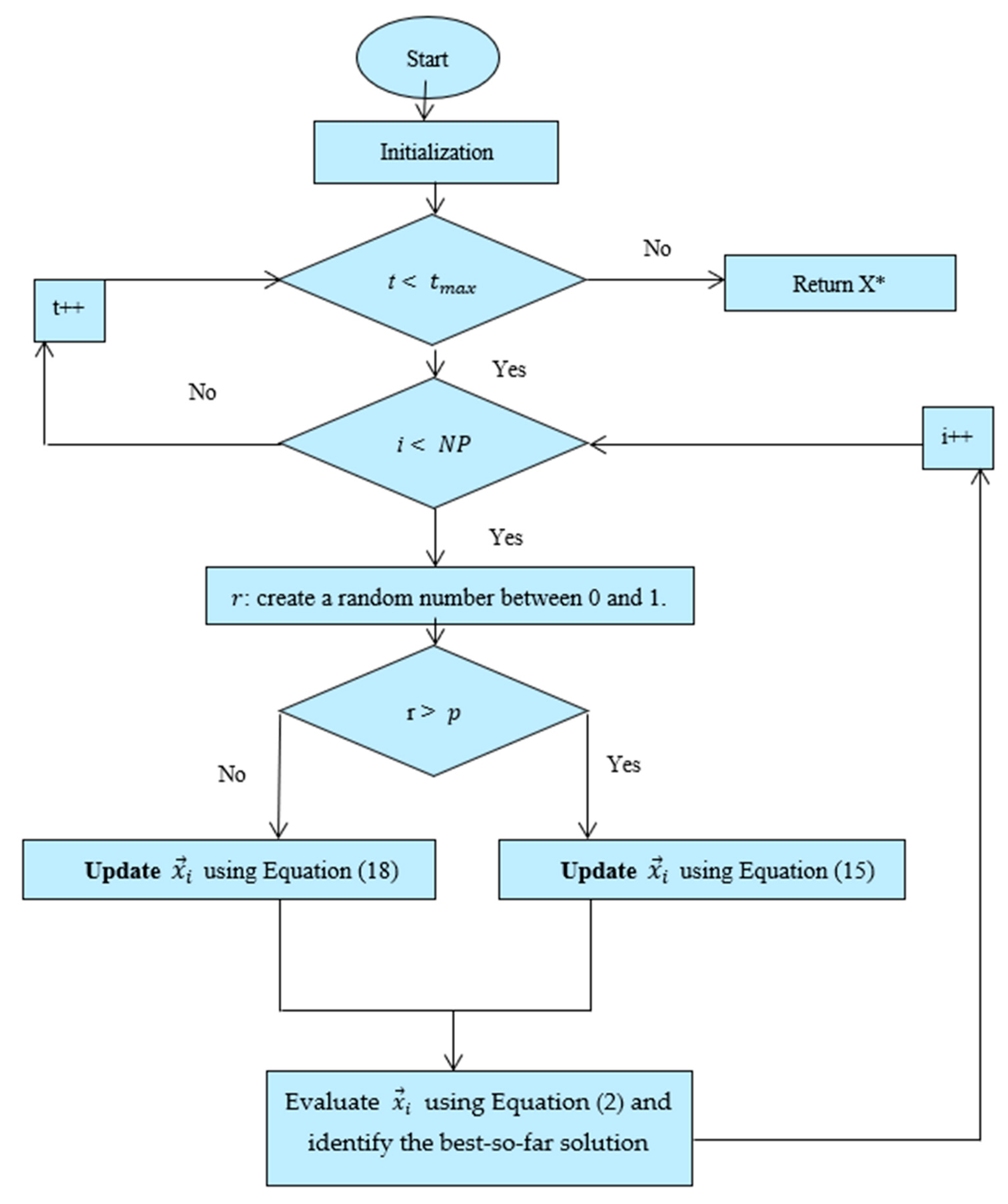
Figure 3.
Framework of the proposed algorithm: HFPA.

Figure 4.
Sensitivity analysis for the parameters of the proposed algorithms: (a) Depiction of outcomes under various values for parameter p on F1; (b) Depiction of outcomes under various values for parameter p on F5; (c) Depiction of outcomes under various values for parameters a on F14; (d) Depiction of outcomes under various values for parameters p₁ on F14.

Figure 5.
The landscape of the mathematical test functions: (a) The landscape of F1; (b) The landscape of F2; (c) The landscape of F3; (d) The landscape of F4; (e) The landscape of F5; (f) The landscape of F6; (g) The landscape of F7; (h) The landscape of F8; (i) The landscape of F9; (j) The landscape of F10; (k) The landscape of F11; (l) The landscape of F12; (m) The landscape of F13; (n) The landscape of F14; (o) The landscape of F15; (p) The landscape of F16; (q) The landscape of F17; (r) The landscape of F18; (s) The landscape of F19; (t) The landscape of F20; (u) The landscape of F21; (v) The landscape of F22; (w) The landscape of F23.


Figure 6.
Outperformance and competitiveness percentage of each algorithm in terms of best and average values on global test functions.
Figure 6.
Outperformance and competitiveness percentage of each algorithm in terms of best and average values on global test functions.

Figure 7.
Convergence curve for unimodal and multimodal benchmark functions: (a) Convergence curve for F1; (b) Convergence curve for F2; (c) Convergence curve for F3; (d) Convergence curve for F6; (e) Convergence curve for F7; (f) Convergence curve for F12; (g) Convergence curve for F19; (h) Convergence curve for F20; (i) Convergence curve for F22.


Figure 8.
Comparison in term of CPU time on global optimization problems.

Figure 9.
Outperformance and competitiveness percentage of each algorithm in terms of best and average values on NESs.
Figure 9.
Outperformance and competitiveness percentage of each algorithm in terms of best and average values on NESs.
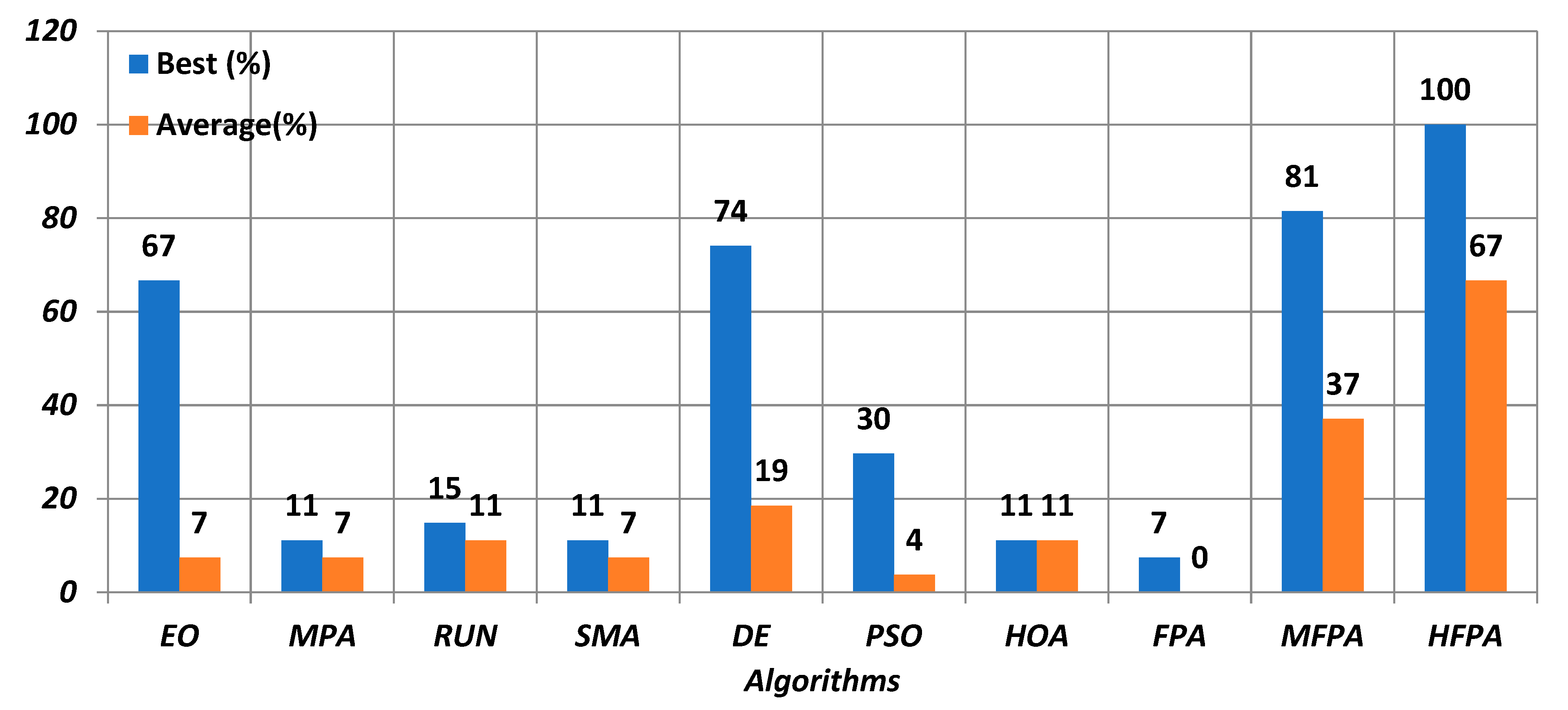
Figure 10.
Convergence curve for the NESs: (a) Convergence curve for f1; (b) Convergence curve for f2; (c) Convergence curve for f3; (d) Convergence curve for f4; (e) Convergence curve for f5; (f) Convergence curve for f7; (g) Convergence curve for f8; (h) Convergence curve for f9; (i) Convergence curve for f10; (j) Convergence curve for f11; (k) Convergence curve for f12; (l) Convergence curve for f13; (m) Convergence curve for f14; (b) Convergence curve for f1; (n) Convergence curve for f15; (o) Convergence curve for f17.
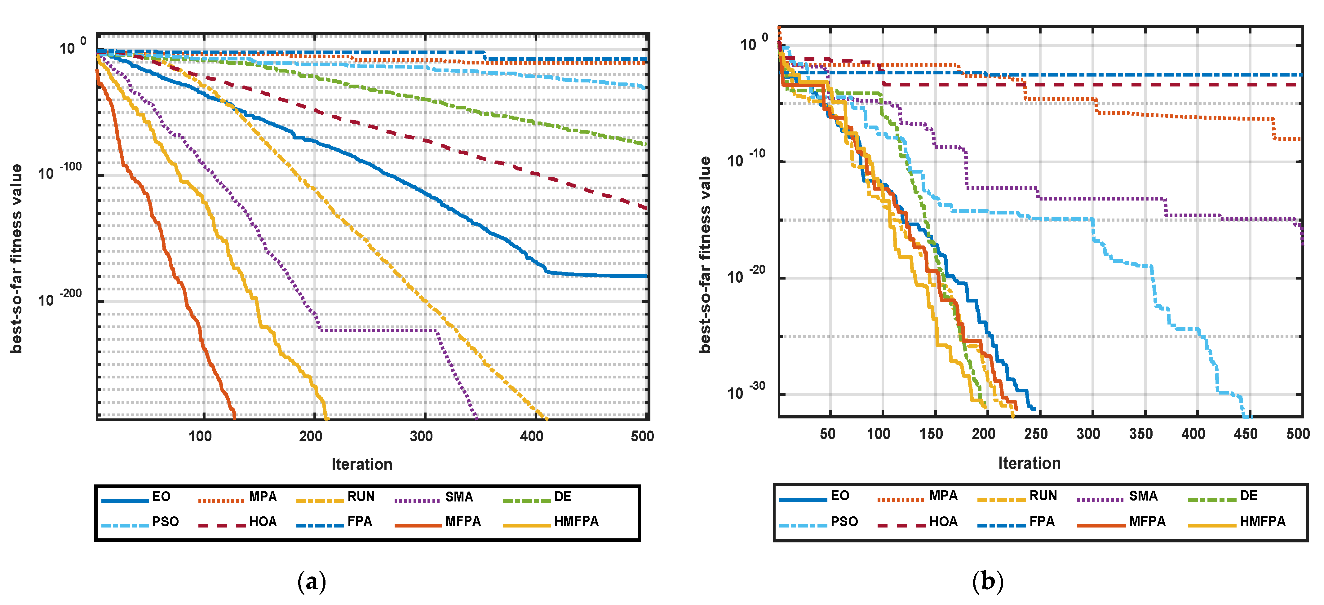
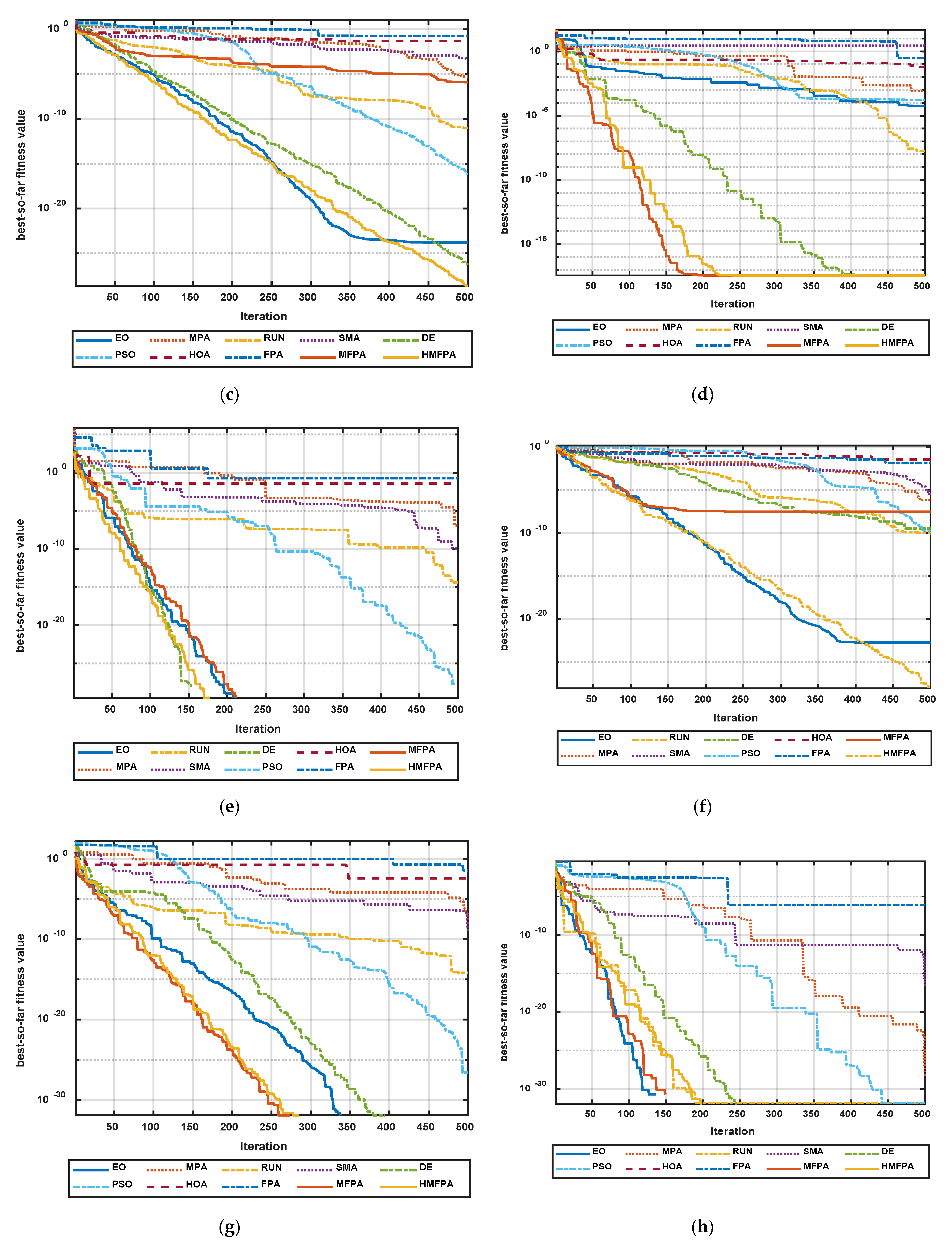


Figure 11.
Comparison in terms of CPU time on NESs.

Figure 12.
Comparison among FPA variants under Boxplot: (a) Boxplot for f1; (b) Boxplot for f2; (c) Boxplot for f3; (d) Boxplot for f5; (e) Boxplot for f6; (f) Boxplot for f7; (g) Boxplot for f8; (h) Boxplot for f9; (i) Boxplot for f10; (j) Boxplot for f11; (k) Boxplot for f12; (l) Boxplot for f13.
Figure 12.
Comparison among FPA variants under Boxplot: (a) Boxplot for f1; (b) Boxplot for f2; (c) Boxplot for f3; (d) Boxplot for f5; (e) Boxplot for f6; (f) Boxplot for f7; (g) Boxplot for f8; (h) Boxplot for f9; (i) Boxplot for f10; (j) Boxplot for f11; (k) Boxplot for f12; (l) Boxplot for f13.

Table 1.
Descriptions of benchmark test functions.
| Name | Formula | D | |
|---|---|---|---|
| Unimodal Test Functions | |||
| Beale | 2 | ||
| Matyas | 2 | ||
| Three-hump camel | 2 | ||
| Exponential | 30 | ||
| Ridge | 30 | ||
| Sphere | 30 | ||
| Step | 30 | ||
| Multimodal Test Functions | |||
| Drop wave | 2 | ||
| Egg holder | 2 | ||
| Himmelblau | 2 | ||
| Levi 13 | 2 | ||
| Ackley 1 | 20 | ||
| Griewank | 5 | ||
| Happy cat | 30 | ||
| Michalewicz | 10 | ||
| Penalized 1 | 30 | ||
| Penalized 2 | 30 | ||
| Periodic | 30 | ||
| Qing | 30 | ||
| Rastrigin | 30 | ||
| Rosenbrock | 30 | ||
| Salomon | 30 | ||
| Yang 4 | 30 | ||
Table 2.
The descriptions of used NESs.
| Function | Formulas | D | References | |
|---|---|---|---|---|
| f1 | 2 | [100] | ||
| f2 | 2 | [100] | ||
| f3 | 10 | [77] | ||
| f4 | 4 | [95] | ||
| f5 | 2 | [101] | ||
| f6 | 2 | [102] | ||
| f7 | 8 | [52] | ||
| f8 | 3 | [103] | ||
| f9 | 2 | [95] | ||
| f10 | 2 | [104] | ||
| f11 | 2 | [104] | ||
| f12 | 20 | [100] | ||
| f13 | 5 | [105] | ||
| f14 | 5 | [106] | ||
| f15 | 20 | [106] | ||
| f16 | 2 | [106] | ||
| f17 | 3 | [106] | ||
| f18 | 3 | [107] | ||
| f19 | 2 | [52] | ||
| f20 | 2 | [52] | ||
| f21 | 2 | [52] | ||
| f22 | 3 | [52] | ||
| f23 | 2 | [52] | ||
| f24 | 2 | [52] | ||
| f25 | 2 | [52] | ||
| f26 | 2 | [52] | ||
| f27 | 2 | [52] |
Table 3.
Comparison under the unimodal mathematical test functions.
| F | EO | MPA | RUN | SMA | DE | PSO | HOA | FPA | MFPA | HFPA | |
|---|---|---|---|---|---|---|---|---|---|---|---|
| F1 | Best | 0 | 6.34 × 10⁻⁸ | 9.23 × 10⁻¹⁹ | 3.07 × 10⁻¹¹ | 0 | 1.26 × 10⁻²⁹ | 5.64 × 10⁻⁵ | 2.23 × 10⁻³ | 0 | 0 |
| Avg | 9.24 × 10⁻³⁴ | 2.37 × 10⁻⁵ | 2.36 × 10⁻¹³ | 1.28 × 10⁻⁸ | 0 | 1.02 × 10⁻¹ | 2.33 × 10⁻² | 1.47 × 10⁻¹ | 0 | 0 | |
| Worst | 2.77 × 10⁻³² | 1.94 × 10⁻⁴ | 2.19 × 10⁻¹² | 1.17 × 10⁻⁷ | 0 | 7.62 × 10⁻¹ | 1.02 × 10⁻¹ | 1.01 | 0 | 0 | |
| SD | 5.06 × 10⁻³³ | 3.91 × 10⁻⁵ | 4.56 × 10⁻¹³ | 2.70 × 10⁻⁸ | 0 | 2.63 × 10⁻¹ | 2.71 × 10⁻² | 2.90 × 10⁻¹ | 0 | 0 | |
| F2 | Best | 4.14 × 10−176 | 8. × 10−12 | 0 | 0 | 7.09 × 10−85 | 1.01 × 10⁻³¹ | 2.79 × 10−137 | 1.54 × 10⁻⁴ | 0 | 0 |
| Avg | 4.60 × 10−130 | 1.78 × 10⁻⁸ | 0 | 1.1 × 10−318 | 1.06 × 10−80 | 2.01 × 10⁻²⁷ | 5.71 × 10⁻⁵ | 8.98 × 10⁻³ | 0 | 0 | |
| Worst | 1.38 × 10−128 | 1.11 × 10⁻⁷ | 0 | 3.5 × 10−317 | 2.12 × 10−79 | 2.40 × 10⁻²⁶ | 1.37 × 10⁻³ | 3.70 × 10⁻² | 0 | 0 | |
| SD | 2.52 × 10−129 | 2.37 × 10⁻⁸ | 0 | 0 | 3.90 × 10−80 | 5.21 × 10⁻²⁷ | 2.50 × 10⁻⁴ | 8.90 × 10⁻³ | 0 | 0 | |
| F3 | Best | 4.12 × 10−247 | 1.56 × 10⁻²⁶ | 0 | 0 | 4.61 × 10−120 | 1.09 × 10⁻³⁴ | 3.10 × 10−256 | 1.26 × 10⁻⁴ | 0 | 0 |
| Avg | 1.61 × 10−198 | 2.66 × 10⁻⁹ | 0 | 0 | 6.20 × 10−112 | 9.95 × 10⁻³ | 5.04 × 10−77 | 3.53 × 10⁻² | 0 | 0 | |
| Worst | 4.83 × 10−197 | 1.79 × 10⁻⁸ | 0 | 0 | 7.57 × 10−111 | 2.99 × 10⁻¹ | 1.51 × 10−75 | 2.36 × 10⁻¹ | 0 | 0 | |
| SD | 0 | 4.48 × 10⁻⁹ | 0 | 0 | 1.97 × 10−111 | 5.45 × 10⁻² | 2.76 × 10−76 | 5.18 × 10⁻² | 0 | 0 | |
| F4 | Best | −1.0000 | −1.0000 | −1.0000 | −1.0000 | −1.0000 | −1.0000 | −1.0000 | −6.58 × 10⁻¹ | −1.0000 | −1.0000 |
| Avg | −1.0000 | −9.90 × 10⁻¹ | −1.0000 | −1.0000 | −1.0000 | −1.0000 | −1.0000 | −2.92 × 10⁻¹ | −1.0000 | −1.0000 | |
| Worst | −1.0000 | −9.68 × 10⁻¹ | −1.0000 | −1.0000 | −1.0000 | −1.0000 | −1.0000 | −6.46 × 10⁻² | −1.0000 | −1.0000 | |
| SD | 5.45 × 10⁻¹⁷ | 9.64 × 10⁻³ | 0 | 0 | 6.94 × 10⁻⁹ | 1.21 × 10⁻⁸ | 6.84 × 10⁻¹⁷ | 1.50 × 10⁻¹ | 0 | 0 | |
| F5 | Best | −5.0000 | −3.42 | −5.0000 | −4.98 | −4.57 | −4.47 | −3.14 | −1.85 | −4.51 | −4.75 |
| Avg | −5.0000 | −2.86 | −5.0000 | −4.96 | −4.54 | −4.22 | −2.85 | −1.67 | −4.22 | −4.67 | |
| Worst | −5.0000 | −2.40 | −5.0000 | −4.93 | −4.48 | −2.85 | −2.70 | −1.54 | −3.86 | −4.61 | |
| SD | 5.79 × 10⁻⁴ | 2.63 × 10⁻¹ | 5.73 × 10⁻⁷ | 1.61 × 10⁻² | 2.34 × 10⁻² | 3.39 × 10⁻¹ | 1.12 × 10⁻¹ | 7.98 × 10⁻² | 1.55 × 10⁻¹ | 3.60 × 10⁻² | |
| F6 | Best | 1.97 × 10−43 | 2.83 × 10⁻² | 3.33 × 10−190 | 0 | 1.05 × 10⁻⁴ | 9.15 × 10⁻⁵ | 3.03 × 10−238 | 1.39 × 10⁴ | 0 | 0 |
| Avg | 1.94 × 10−40 | 3.52 × 10² | 1.56 × 10−163 | 1.3 × 10−319 | 3.50 × 10⁻⁴ | 6.96 × 10⁻⁴ | 1.11 × 10−125 | 2.67 × 10⁴ | 0 | 0 | |
| Worst | 1.65 × 10−39 | 1.39 × 10³ | 4.67 × 10−162 | 4.0 × 10−318 | 8.85 × 10⁻⁴ | 2.72 × 10⁻³ | 3.34 × 10−124 | 6.19 × 10⁴ | 0 | 0 | |
| SD | 3.57 × 10−40 | 3.95 × 10² | 0 | 0 | 1.86 × 10⁻⁴ | 6.35 × 10⁻⁴ | 6.10 × 10−125 | 1.00 × 10⁴ | 0 | 0 | |
| F7 | Best | 1.24 × 10⁻⁶ | 4.61 × 10⁻² | 1.62 × 10⁻⁷ | 1.65 × 10⁻⁵ | 3.24 × 10⁻⁷ | 6.89 × 10⁻⁷ | 4.33 | 2.89 × 10 | 2.98 × 10⁻² | 7.44 × 10⁻⁸ |
| Avg | 5.33 × 10⁻⁶ | 6.91 × 10⁻¹ | 3.28 × 10⁻⁷ | 9.95 × 10⁻⁴ | 8.90 × 10⁻⁷ | 7.39 × 10⁻⁶ | 6.04 | 8.50 × 10 | 5.76 × 10⁻¹ | 2.83 × 10⁻⁶ | |
| Worst | 1.39 × 10⁻⁵ | 3.57 | 5.43 × 10⁻⁷ | 2.91 × 10⁻³ | 2.24 × 10⁻⁶ | 3.72 × 10⁻⁵ | 7.02 | 1.51 × 10² | 1.23 | 2.15 × 10⁻⁵ | |
| SD | 3.11 × 10⁻⁶ | 8.92 × 10⁻¹ | 8.52 × 10⁻⁸ | 8.20 × 10⁻⁴ | 4.67 × 10⁻⁷ | 9.04 × 10⁻⁶ | 7.18 × 10⁻¹ | 3.08 × 10 | 2.97 × 10⁻¹ | 4.36 × 10⁻⁶ | |
| F8 | Best | −1.0000 | −1.0000 | −1.0000 | −1.0000 | −1.0000 | −1.0000 | −1.0000 | −9.92 × 10⁻¹ | −1.0000 | −1.0000 |
| Avg | −1.0000 | −9.98 × 10⁻¹ | −1.0000 | −1.0000 | −1.0000 | −9.88 × 10⁻¹ | −9.99 × 10⁻¹ | −9.11 × 10⁻¹ | −1.0000 | −1.0000 | |
| Worst | −1.0000 | −9.36 × 10⁻¹ | −1.0000 | −1.0000 | −1.0000 | −9.36 × 10⁻¹ | −9.77 × 10⁻¹ | −7.82 × 10⁻¹ | −1.0000 | −1.0000 | |
| SD | 0 | 1.16 × 10⁻² | 0 | 0 | 0 | 2.18 × 10⁻² | 4.39 × 10⁻³ | 4.71 × 10⁻² | 0 | 0 |
Bold values indicate the best outcomes.
Table 4.
Comparison under the multimodal mathematical test functions.
| F | EO | MPA | RUN | SMA | DE | PSO | HOA | FPA | MFPA | HFPA | |
|---|---|---|---|---|---|---|---|---|---|---|---|
| F9 | Best | −9.60 × 10² | −9.60 × 10² | −9.60 × 10² | −9.60 × 10² | −9.60 × 10² | −9.60 × 10² | −9.60 × 10² | −9.60 × 10² | −9.60 × 10² | −9.60 × 10² |
| Avg | −9.52 × 10² | −9.60 × 10² | −9.60 × 10² | −9.60 × 10² | −9.53 × 10² | −7.60 × 10² | −8.98 × 10² | −9.18 × 10² | −9.10 × 10² | −9.28 × 10² | |
| Worst | −7.87 × 10² | −9.60 × 10² | −9.60 × 10² | −9.60 × 10² | −8.21 × 10² | −5.25 × 10² | −7.18 × 10² | −7.79 × 10² | −7.17 × 10² | −7.18 × 10² | |
| SD | 3.34 × 10 | 5.78 × 10⁻¹³ | 1.47 × 10⁻⁹ | 1.47 × 10⁻⁸ | 2.71 × 10 | 1.04 × 10² | 6.77 × 10 | 5.60 × 10 | 7.41 × 10 | 6.25 × 10 | |
| F10 | Best | 0 | 2.88 × 10⁻⁹ | 1.17 × 10⁻¹⁸ | 1.24 × 10⁻⁹ | 0 | 0 | 0 | 3.76 × 10⁻³ | 0 | 0 |
| Avg | 1.15 × 10⁻³¹ | 8.24 × 10⁻⁶ | 2.90 × 10⁻¹¹ | 1.82 × 10⁻⁷ | 1.05 × 10⁻³¹ | 6.27 × 10⁻²⁷ | 1.57 × 10⁻³ | 2.68 × 10⁻¹ | 3.16 × 10⁻³¹ | 1.05 × 10⁻³¹ | |
| Worst | 7.89 × 10⁻³¹ | 8.05 × 10⁻⁵ | 1.94 × 10⁻¹⁰ | 6.35 × 10⁻⁷ | 7.89 × 10⁻³¹ | 1.16 × 10⁻²⁵ | 1.05 × 10⁻² | 1.87 | 7.89 × 10⁻³¹ | 7.89 × 10⁻³¹ | |
| SD | 2.77 × 10⁻³¹ | 1.74 × 10⁻⁵ | 4.73 × 10⁻¹¹ | 2.00 × 10⁻⁷ | 2.73 × 10⁻³¹ | 2.17 × 10⁻²⁶ | 2.45 × 10⁻³ | 4.04 × 10⁻¹ | 3.93 × 10⁻³¹ | 2.73 × 10⁻³¹ | |
| F11 | Best | 1.35 × 10⁻³¹ | 1.97 × 10⁻¹⁰ | 1.61 × 10⁻¹⁷ | 5.03 × 10⁻¹³ | 1.35 × 10⁻³¹ | 2.23 × 10⁻³⁰ | 2.72 × 10⁻³ | 3.75 × 10⁻³ | 1.35 × 10⁻³¹ | 1.35 × 10⁻³¹ |
| Avg | 1.35 × 10⁻³¹ | 4.65 × 10⁻⁶ | 1.26 × 10⁻¹¹ | 3.68 × 10⁻⁹ | 1.35 × 10⁻³¹ | 2.30 × 10⁻²⁵ | 1.74 × 10⁻¹ | 3.15 × 10⁻¹ | 1.35 × 10⁻³¹ | 1.35 × 10⁻³¹ | |
| Worst | 1.35 × 10⁻³¹ | 6.73 × 10⁻⁵ | 8.72 × 10⁻¹¹ | 2.31 × 10⁻⁸ | 1.35 × 10⁻³¹ | 6.62 × 10⁻²⁴ | 3.63 × 10⁻¹ | 7.91 × 10⁻¹ | 1.35 × 10⁻³¹ | 1.35 × 10⁻³¹ | |
| SD | 6.68 × 10−47 | 1.26 × 10⁻⁵ | 2.13 × 10⁻¹¹ | 5.21 × 10⁻⁹ | 6.68 × 10−47 | 1.21 × 10⁻²⁴ | 9.32 × 10⁻² | 2.28 × 10⁻¹ | 6.68 × 10−47 | 6.68 × 10−47 | |
| F12 | Best | 4.44 × 10⁻¹⁵ | 3.65 | 8.88 × 10⁻¹⁶ | 8.88 × 10⁻¹⁶ | 2.64 × 10⁻³ | 2.12 | 4.44 × 10⁻¹⁵ | 1.59 × 10 | 8.88 × 10⁻¹⁶ | 8.88 × 10⁻¹⁶ |
| Avg | 9.06 × 10⁻¹⁵ | 6.60 | 8.88 × 10⁻¹⁶ | 8.88 × 10⁻¹⁶ | 5.25 × 10⁻³ | 6.28 | 6.57 × 10⁻¹⁵ | 1.89 × 10 | 8.88 × 10⁻¹⁶ | 8.88 × 10⁻¹⁶ | |
| Worst | 1.51 × 10⁻¹⁴ | 1.15 × 10 | 8.88 × 10⁻¹⁶ | 8.88 × 10⁻¹⁶ | 9.38 × 10⁻³ | 8.91 | 1.51 × 10⁻¹⁴ | 2.06 × 10 | 8.88 × 10⁻¹⁶ | 8.88 × 10⁻¹⁶ | |
| SD | 2.97 × 10⁻¹⁵ | 2.22 | 0 | 0 | 1.74 × 10⁻³ | 1.61 | 2.57 × 10⁻¹⁵ | 1.46 | 0 | 0 | |
| F13 | Best | 4.38 × 10⁻³ | 1.24 | 9.44 × 10⁻⁵ | 3.45 × 10⁻² | 3.54 × 10⁻⁴ | 3.71 × 10⁻³ | 1.06 × 10 | 1.41 × 10² | 1.11 | 1.87 × 10⁻⁴ |
| Avg | 2.61 × 10⁻² | 7.75 | 1.25 × 10⁻² | 5.54 × 10⁻¹ | 1.57 × 10⁻² | 6.23 × 10⁻² | 3.69 × 10 | 2.69 × 10² | 5.17 | 2.89 × 10⁻² | |
| Worst | 8.88 × 10⁻² | 2.54 × 10 | 4.67 × 10⁻² | 9.88 × 10⁻¹ | 1.18 × 10⁻¹ | 4.49 × 10⁻¹ | 6.61 × 10 | 4.64 × 10² | 1.32 × 10 | 1.18 × 10⁻¹ | |
| SD | 2.44 × 10⁻² | 5.84 | 1.32 × 10⁻² | 3.57 × 10⁻¹ | 2.85 × 10⁻² | 9.00 × 10⁻² | 1.88 × 10 | 7.68 × 10 | 2.69 | 2.60 × 10⁻² | |
| F14 | Best | 2.04 × 10⁻¹ | 3.88 × 10⁻¹ | 1.26 × 10⁻¹ | 1.59 × 10⁻¹ | 3.54 × 10⁻¹ | 5.05 × 10⁻¹ | 1.05 | 8.42 × 10⁻¹ | 4.52 × 10⁻¹ | 2.67 × 10⁻¹ |
| Avg | 3.42 × 10⁻¹ | 7.10 × 10⁻¹ | 2.48 × 10⁻¹ | 4.12 × 10⁻¹ | 5.38 × 10⁻¹ | 7.09 × 10⁻¹ | 1.45 | 1.37 | 6.93 × 10⁻¹ | 5.19 × 10⁻¹ | |
| Worst | 5.61 × 10⁻¹ | 9.08 × 10⁻¹ | 3.85 × 10⁻¹ | 7.12 × 10⁻¹ | 6.73 × 10⁻¹ | 9.82 × 10⁻¹ | 1.99 | 1.76 | 1.01 | 7.29 × 10⁻¹ | |
| SD | 8.06 × 10⁻² | 1.08 × 10⁻¹ | 6.57 × 10⁻² | 1.54 × 10⁻¹ | 7.85 × 10⁻² | 1.20 × 10⁻¹ | 2.33 × 10⁻¹ | 2.23 × 10⁻¹ | 1.51 × 10⁻¹ | 1.01 × 10⁻¹ | |
| F15 | Best | −9.58 | −7.86 | −9.36 | −9.36 | −9.60 | −9.14 | −6.00 | −5.47 | −8.95 | −9.66 |
| Avg | −8.50 | −5.99 | −8.06 | −7.73 | −9.20 | −7.53 | −5.17 | −3.72 | −7.30 | −9.39 | |
| Worst | −7.07 | −4.61 | −6.74 | −6.32 | −8.15 | −5.05 | −4.46 | −2.97 | −5.53 | −8.71 | |
| SD | 7.23 × 10⁻¹ | 8.40 × 10⁻¹ | 7.53 × 10⁻¹ | 9.51 × 10⁻¹ | 2.30 × 10⁻¹ | 1.14 | 4.37 × 10⁻¹ | 5.62 × 10⁻¹ | 9.19 × 10⁻¹ | 2.00 × 10⁻¹ | |
| F16 | Best | 3.77 × 10⁻⁸ | 3.27 × 10⁻¹ | 6.52 × 10⁻⁹ | 2.00 × 10⁻⁶ | 6.79 × 10⁻⁵ | 2.62 × 10⁻⁵ | 8.64 × 10⁻¹ | 1.12 × 10⁶ | 9.66 × 10⁻³ | 6.40 × 10⁻⁹ |
| Avg | 3.46 × 10⁻³ | 3.25 × 10³ | 2.06 × 10⁻⁷ | 5.17 × 10⁻³ | 5.44 × 10⁻⁴ | 1.17 | 1.30 | 1.08 × 10⁸ | 3.40 × 10⁻² | 6.97 × 10⁻⁸ | |
| Worst | 1.04 × 10⁻¹ | 9.37 × 10⁴ | 4.16 × 10⁻⁶ | 2.50 × 10⁻² | 4.66 × 10⁻³ | 3.42 | 3.22 | 4.46 × 10⁸ | 5.97 × 10⁻² | 2.61 × 10⁻⁷ | |
| SD | 1.89 × 10⁻² | 1.71 × 10⁴ | 8.19 × 10⁻⁷ | 6.63 × 10⁻³ | 8.57 × 10⁻⁴ | 9.25 × 10⁻¹ | 4.17 × 10⁻¹ | 1.20 × 10⁸ | 1.41 × 10⁻² | 8.19 × 10⁻⁸ | |
| F17 | Best | 2.69 × 10⁻⁶ | 4.17 × 10⁻¹ | 1.31 × 10⁻⁸ | 1.84 × 10⁻⁴ | 1.90 × 10⁻⁴ | 5.41 × 10⁻¹ | 2.86 | 1.24 × 10⁷ | 2.58 | 1.18 |
| Avg | 4.26 × 10⁻² | 4.73 × 10³ | 6.13 × 10⁻³ | 4.25 × 10⁻³ | 1.71 × 10⁻³ | 1.26 × 10 | 3.04 | 1.69 × 10⁸ | 2.80 | 2.28 | |
| Worst | 1.96 × 10⁻¹ | 5.57 × 10⁴ | 2.10 × 10⁻² | 1.62 × 10⁻² | 8.23 × 10⁻³ | 2.87 × 10 | 3.46 | 8.03 × 10⁸ | 2.97 | 2.97 | |
| SD | 5.47 × 10⁻² | 1.37 × 10⁴ | 7.25 × 10⁻³ | 3.44 × 10⁻³ | 1.75 × 10⁻³ | 6.13 | 1.28 × 10⁻¹ | 1.67 × 10⁸ | 1.22 × 10⁻¹ | 4.94 × 10⁻¹ | |
| F18 | Best | 2.74 | 2.07 | 9.00 × 10⁻¹ | 9.00 × 10⁻¹ | 1.71 | 5.73 | 2.95 | 3.02 | 9.00 × 10⁻¹ | 9.00 × 10⁻¹ |
| Avg | 2.86 | 2.47 | 1.10 | 9.11 × 10⁻¹ | 2.02 | 7.40 | 3.05 | 4.64 | 9.00 × 10⁻¹ | 9.00 × 10⁻¹ | |
| Worst | 3.00 | 2.74 | 2.91 | 1.00 | 2.34 | 9.37 | 3.07 | 7.11 | 9.00 × 10⁻¹ | 9.00 × 10⁻¹ | |
| SD | 5.08 × 10⁻² | 1.57 × 10⁻¹ | 5.27 × 10⁻¹ | 3.05 × 10⁻² | 1.40 × 10⁻¹ | 8.65 × 10⁻¹ | 2.87 × 10⁻² | 1.36 | 4.52 × 10⁻¹⁶ | 4.52 × 10⁻¹⁶ | |
| F19 | Best | 5.38 × 10⁻³ | 3.05 × 10³ | 3.52 × 10⁻³ | 2.41 | 8.69 × 10² | 3.27 × 10⁻² | 6.23 × 10³ | 1.59 × 10⁹ | 1.22 × 10² | 1.79 × 10⁻⁴ |
| Avg | 5.44 × 10⁻¹ | 4.50 × 10⁷ | 3.37 × 10⁻¹ | 5.82 | 1.38 × 10³ | 5.20 × 10⁻¹ | 7.46 × 10³ | 4.63 × 10¹⁰ | 5.97 × 10² | 1.05 × 10⁻¹ | |
| Worst | 8.69 | 4.76 × 10⁸ | 3.90 | 1.71 × 10 | 1.81 × 10³ | 8.14 | 8.54 × 10³ | 1.87 × 10¹¹ | 1.49 × 10³ | 2.78 | |
| SD | 1.70 | 9.89 × 10⁷ | 9.68 × 10⁻¹ | 3.59 | 2.45 × 10² | 1.47 | 5.83 × 10² | 3.87 × 10¹⁰ | 3.96 × 10² | 5.06 × 10⁻¹ | |
| F20 | Best | 0 | 4.05 × 10 | 0 | 0 | 1.22 × 10² | 1.82 × 10 | 0 | 2.97 × 10² | 0 | 0 |
| Avg | 0 | 9.56 × 10 | 0 | 0 | 1.54 × 10² | 9.48 × 10 | 2.28 × 10 | 3.69 × 10² | 0 | 0 | |
| Worst | 0 | 1.63 × 10² | 0 | 0 | 1.74 × 10² | 2.29 × 10² | 2.44 × 10² | 4.26 × 10² | 0 | 0 | |
| SD | 0 | 3.11 × 10 | 0 | 0 | 1.16 × 10 | 7.06 × 10 | 7.00 × 10 | 3.73 × 10 | 0 | 0 | |
| F21 | Best | 2.48 × 10 | 2.53 × 10² | 2.41 × 10 | 6.95 × 10⁻³ | 2.55 × 10 | 6.15 × 10⁻² | 2.87 × 10 | 1.35 × 10⁵ | 2.58 × 10 | 2.23 × 10 |
| Avg | 2.54 × 10 | 2.12 × 10³ | 2.56 × 10 | 3.88 × 10⁻¹ | 3.03 × 10 | 8.14 × 10 | 2.89 × 10 | 4.40 × 10⁵ | 2.68 × 10 | 2.36 × 10 | |
| Worst | 2.60 × 10 | 5.16 × 10³ | 2.87 × 10 | 1.35 | 9.32 × 10 | 3.17 × 10² | 2.90 × 10 | 1.08 × 10⁶ | 2.84 × 10 | 2.50 × 10 | |
| SD | 3.19 × 10⁻¹ | 1.53 × 10³ | 1.13 | 3.44 × 10⁻¹ | 1.30 × 10 | 7.43 × 10 | 6.73 × 10⁻² | 2.36 × 10⁵ | 6.16 × 10⁻¹ | 7.38 × 10⁻¹ | |
| F22 | Best | 9.99 × 10⁻² | 1.30 | 1.14 × 10−84 | 0 | 6.21 × 10⁻¹ | 3.10 | 2.00 × 10⁻¹ | 8.89 | 0 | 0 |
| Avg | 1.03 × 10⁻¹ | 4.28 | 8.72 × 10−64 | 6.30 × 10−145 | 7.94 × 10⁻¹ | 4.43 | 8.42 × 10⁻¹ | 1.74 × 10 | 0 | 0 | |
| Worst | 2.00 × 10⁻¹ | 9.00 | 2.61 × 10−62 | 1.89 × 10−143 | 1.01 | 5.70 | 2.47 | 2.50 × 10 | 0 | 0 | |
| SD | 1.83 × 10⁻² | 1.93 | 4.76 × 10−63 | 3.45 × 10−144 | 9.74 × 10⁻² | 7.60 × 10⁻¹ | 4.76 × 10⁻¹ | 3.42 | 0 | 0 | |
| F23 | Best | 1.78 × 10⁻¹⁷ | 3.70 × 10⁻¹⁵ | −1.0000 | −1.0000 | 2.50 × 10⁻¹² | 5.99 × 10⁻¹⁴ | 1.36 × 10⁻¹² | 3.34 × 10⁻¹⁰ | −1.0000 | −1.0000 |
| Avg | 2.08 × 10⁻¹⁶ | 6.68 × 10⁻¹³ | −1.0000 | −1.0000 | 5.60 × 10⁻¹² | 7.81 × 10⁻¹² | 9.00 × 10⁻¹² | 5.45 × 10⁻⁹ | −1.0000 | −1.0000 | |
| Worst | 5.79 × 10⁻¹⁶ | 4.66 × 10⁻¹² | −1.0000 | −1.0000 | 1.21 × 10⁻¹¹ | 5.97 × 10⁻¹¹ | 2.45 × 10⁻¹¹ | 2.36 × 10⁻⁸ | −1.0000 | −1.0000 | |
| SD | 1.59 × 10⁻¹⁶ | 1.16 × 10⁻¹² | 0 | 0 | 2.04 × 10⁻¹² | 1.43 × 10⁻¹¹ | 4.89 × 10⁻¹² | 6.06 × 10⁻⁹ | 0 | 0 |
Bold values indicate the best outcomes.
Table 5.
Comparison on test cases f1–f13.
| F | EO | MPA | RUN | SMA | DE | PSO | HOA | FPA | MFPA | HFPA | |
|---|---|---|---|---|---|---|---|---|---|---|---|
| f1 | Best | 8.0 × 10−183 | 3.39 × 10⁻¹⁴ | 0 | 0 | 9.75 × 10−86 | 5.55 × 10⁻³² | 1.1 × 10−128 | 4.31 × 10⁻⁵ | 0 | 0 |
| Avg | 1.36 × 10⁻¹⁰ | 2.15 × 10⁻⁶ | 1.21 × 10−47 | 9.3 × 10−312 | 1.73 × 10⁻³² | 3.78 × 10⁻¹⁵ | 3.71 × 10⁻⁵ | 1.42 × 10⁻³ | 0 | 0 | |
| Worst | 4.09 × 10⁻⁹ | 2.93 × 10⁻⁵ | 3.63 × 10−46 | 2.7 × 10−310 | 2.47 × 10⁻³² | 1.06 × 10⁻¹³ | 1.72 × 10⁻⁴ | 1.05 × 10⁻² | 0 | 0 | |
| SD | 7.46 × 10⁻¹⁰ | 5.70 × 10⁻⁶ | 6.63 × 10−47 | 0 | 1.09 × 10⁻³² | 1.93 × 10⁻¹⁴ | 4.96 × 10⁻⁵ | 2.08 × 10⁻³ | 0 | 0 | |
| f2 | Best | 0 | 2.93 × 10⁻⁹ | 0 | 1.25 × 10⁻¹⁷ | 0 | 0 | 2.54 × 10⁻⁵ | 2.49 × 10⁻⁴ | 0 | 0 |
| Avg | 4.63 × 10⁻²⁵ | 4.09 × 10⁻⁶ | 4.78 × 10⁻¹² | 3.16 × 10⁻⁹ | 5.81 × 10⁻³² | 4.45 × 10⁻²⁵ | 4.11 × 10⁻³ | 7.00 × 10⁻² | 5.87 × 10⁻³² | 3.52 × 10⁻³² | |
| Worst | 1.39 × 10⁻²³ | 2.73 × 10⁻⁵ | 6.41 × 10⁻¹¹ | 6.15 × 10⁻⁸ | 2.74 × 10⁻³¹ | 1.24 × 10⁻²³ | 2.28 × 10⁻² | 2.55 × 10⁻¹ | 3.08 × 10⁻³¹ | 2.74 × 10⁻³¹ | |
| SD | 2.54 × 10⁻²⁴ | 6.37 × 10⁻⁶ | 1.48 × 10⁻¹¹ | 1.12 × 10⁻⁸ | 1.10 × 10⁻³¹ | 2.26 × 10⁻²⁴ | 4.67 × 10⁻³ | 6.37 × 10⁻² | 1.06 × 10⁻³¹ | 8.20 × 10⁻³² | |
| f3 | Best | 2.11 × 10⁻²³ | 1.76 × 10⁻⁶ | 9.38 × 10⁻¹² | 1.30 × 10⁻⁴ | 3.62 × 10⁻²⁷ | 1.25 × 10⁻¹⁶ | 8.89 × 10⁻² | 6.91 × 10⁻¹ | 1.80 × 10⁻⁶ | 8.65 × 10⁻³⁰ |
| Avg | 1.44 × 10⁻¹⁹ | 5.60 × 10⁻⁵ | 7.91 × 10⁻¹⁰ | 2.53 × 10⁻³ | 1.12 × 10⁻²⁵ | 1.50 × 10⁻¹⁴ | 1.83 × 10⁻¹ | 1.68 | 4.31 × 10⁻⁵ | 1.96 × 10⁻²⁶ | |
| Worst | 3.00 × 10⁻¹⁸ | 3.32 × 10⁻⁴ | 5.00 × 10⁻⁹ | 8.72 × 10⁻³ | 1.09 × 10⁻²⁴ | 1.39 × 10⁻¹³ | 3.89 × 10⁻¹ | 3.76 | 1.81 × 10⁻⁴ | 3.20 × 10⁻²⁵ | |
| SD | 5.54 × 10⁻¹⁹ | 7.18 × 10⁻⁵ | 1.15 × 10⁻⁹ | 2.35 × 10⁻³ | 2.19 × 10⁻²⁵ | 2.92 × 10⁻¹⁴ | 7.34 × 10⁻² | 8.07 × 10⁻¹ | 5.15 × 10⁻⁵ | 5.87 × 10⁻²⁶ | |
| f4 | Best | 1.56 × 10⁻⁵ | 3.48 × 10⁻⁵ | 7.08 × 10⁻⁹ | 3.69 × 10⁻¹ | 3.61 × 10⁻¹⁸ | 1.14 × 10⁻⁴ | 4.36 × 10⁻² | 2.47 × 10⁻¹ | 3.61 × 10⁻¹⁸ | 3.61 × 10⁻¹⁸ |
| Avg | 9.20 × 10⁻³ | 5.92 × 10⁻² | 1.78 × 10⁻³ | 4.06 | 2.34 × 10⁻³ | 5.20 × 10⁻² | 2.10 | 2.98 | 1.54 × 10⁻¹ | 6.46 × 10⁻² | |
| Worst | 1.36 × 10⁻² | 1.72 × 10⁻¹ | 1.75 × 10⁻² | 4.36 | 4.92 × 10⁻² | 3.29 × 10⁻¹ | 9.07 | 8.89 | 6.64 × 10⁻¹ | 6.64 × 10⁻¹ | |
| SD | 4.58 × 10⁻³ | 4.96 × 10⁻² | 4.60 × 10⁻³ | 8.05 × 10⁻¹ | 9.36 × 10⁻³ | 1.02 × 10⁻¹ | 2.89 | 2.34 | 2.53 × 10⁻¹ | 1.76 × 10⁻¹ | |
| f5 | Best | 0 | 5.15 × 10⁻⁶ | 7.07 × 10⁻¹⁵ | 7.44 × 10⁻¹¹ | 0 | 2.02 × 10⁻²⁸ | 2.78 × 10⁻¹ | 5.50 × 10⁻¹ | 0 | 0 |
| Avg | 0 | 1.07 × 10⁻² | 1.08 × 10⁻⁸ | 3.12 × 10⁻⁸ | 1.35 × 10⁻²⁹ | 5.22 × 10⁻²³ | 2.03 × 10 | 7.81 × 10 | 6.06 × 10⁻²⁹ | 0 | |
| Worst | 0 | 1.88 × 10⁻¹ | 3.21 × 10⁻⁷ | 4.29 × 10⁻⁷ | 2.02 × 10⁻²⁸ | 1.40 × 10⁻²¹ | 2.32 × 10² | 3.59 × 10² | 8.08 × 10⁻²⁸ | 0 | |
| SD | 0 | 3.49 × 10⁻² | 5.87 × 10⁻⁸ | 7.83 × 10⁻⁸ | 5.12 × 10⁻²⁹ | 2.55 × 10⁻²² | 4.22 × 10 | 8.36 × 10 | 1.60 × 10⁻²⁸ | 0 | |
| f6 | Best | 0 | 0 | 0 | 0 | 0 | 6.17 × 10⁻³² | 0 | 0 | 0 | 0 |
| Avg | 1.36 × 10⁻³² | 0 | 0 | 0 | 1.00 × 10⁻³² | 1.14 × 10⁻²² | 0 | 2.04 × 10⁻³¹ | 0 | 0 | |
| Worst | 3.00 × 10⁻³¹ | 0 | 0 | 0 | 3.00 × 10⁻³¹ | 3.43 × 10⁻²¹ | 0 | 1.08 × 10⁻³⁰ | 0 | 0 | |
| SD | 5.76 × 10⁻³² | 0 | 0 | 0 | 5.48 × 10⁻³² | 6.26 × 10⁻²² | 0 | 3.69 × 10⁻³¹ | 0 | 0 | |
| f7 | Best | 9.99 × 10⁻²⁵ | 2.62 × 10⁻⁷ | 2.23 × 10⁻¹⁰ | 2.63 × 10⁻⁶ | 3.35 × 10⁻⁸ | 2.84 × 10⁻¹² | 3.04 × 10⁻² | 2.13 × 10⁻² | 1.39 × 10⁻⁸ | 1.69 × 10⁻²⁷ |
| Avg | 1.87 × 10⁻¹⁵ | 6.47 × 10⁻³ | 3.17 × 10⁻⁷ | 4.14 × 10⁻³ | 2.04 × 10⁻⁴ | 2.85 × 10⁻² | 2.48 × 10⁻¹ | 1.96 × 10⁻¹ | 2.16 × 10⁻⁵ | 8.08 × 10⁻²⁰ | |
| Worst | 2.00 × 10⁻¹⁴ | 1.03 × 10⁻¹ | 4.48 × 10⁻⁶ | 1.23 × 10⁻¹ | 3.27 × 10⁻³ | 1.42 × 10⁻¹ | 6.40 × 10⁻¹ | 3.87 × 10⁻¹ | 1.76 × 10⁻⁴ | 2.38 × 10⁻¹⁸ | |
| SD | 4.78 × 10⁻¹⁵ | 2.35 × 10⁻² | 1.03 × 10⁻⁶ | 2.25 × 10⁻² | 6.17 × 10⁻⁴ | 4.13 × 10⁻² | 1.54 × 10⁻¹ | 9.36 × 10⁻² | 3.97 × 10⁻⁵ | 4.34 × 10⁻¹⁹ | |
| f8 | Best | 0 | 2.51 × 10⁻⁸ | 6.11 × 10⁻¹⁵ | 5.69 × 10⁻¹⁰ | 0 | 4.28 × 10⁻²⁶ | 1.94 × 10⁻³ | 6.35 × 10⁻² | 0 | 0 |
| Avg | 9.44 × 10⁻²⁴ | 2.65 × 10⁻⁵ | 6.26 × 10⁻¹³ | 6.37 × 10⁻⁸ | 1.19 × 10⁻³² | 6.72 × 10⁻¹ | 1.05 × 10⁻¹ | 3.03 | 6.98 × 10⁻³³ | 9.04 × 10⁻³³ | |
| Worst | 2.83 × 10⁻²² | 2.07 × 10⁻⁴ | 3.20 × 10⁻¹² | 3.35 × 10⁻⁷ | 1.23 × 10⁻³² | 4.03 | 3.87 × 10⁻¹ | 1.56 × 10 | 2.47 × 10⁻³² | 1.23 × 10⁻³² | |
| SD | 5.17 × 10⁻²³ | 4.80 × 10⁻⁵ | 7.56 × 10⁻¹³ | 1.01 × 10⁻⁷ | 2.25 × 10⁻³³ | 1.53 | 8.55 × 10⁻² | 4.09 | 7.01 × 10⁻³³ | 5.54 × 10⁻³³ | |
| f9 | Best | 0 | 9.03 × 10⁻²⁷ | 2.21 × 10⁻²⁹ | 1.27 × 10⁻¹⁶ | 0 | 0 | 0 | 4.96 × 10⁻⁷ | 0 | 0 |
| Avg | 4.50 × 10⁻³³ | 8.78 × 10⁻⁸ | 5.63 × 10⁻¹¹ | 4.34 × 10⁻¹² | 1.50 × 10⁻³³ | 1.94 × 10⁻²² | 0 | 7.69 × 10⁻⁴ | 5.00 × 10⁻³⁴ | 2.00 × 10⁻³³ | |
| Worst | 1.50 × 10⁻³² | 2.63 × 10⁻⁶ | 1.06 × 10⁻⁹ | 9.75 × 10⁻¹¹ | 1.50 × 10⁻³² | 2.80 × 10⁻²¹ | 0 | 6.15 × 10⁻³ | 1.50 × 10⁻³² | 1.50 × 10⁻³² | |
| SD | 6.99 × 10⁻³³ | 4.80 × 10⁻⁷ | 2.19 × 10⁻¹⁰ | 1.78 × 10⁻¹¹ | 4.58 × 10⁻³³ | 6.78 × 10⁻²² | 0 | 1.31 × 10⁻³ | 2.74 × 10⁻³³ | 5.19 × 10⁻³³ | |
| f10 | Best | 0 | 1.88 × 10⁻⁷ | 1.82 × 10⁻¹⁶ | 4.56 × 10⁻¹¹ | 0 | 0 | 2.66 × 10⁻³ | 2.22 × 10⁻² | 0 | 0 |
| Avg | 1.31 × 10⁻³⁰ | 2.01 × 10⁻⁴ | 8.36 × 10⁻¹² | 4.02 × 10⁻⁸ | 0 | 8.71 × 10⁻²⁵ | 3.83 × 10⁻¹ | 4.46 | 1.31 × 10⁻³¹ | 1.05 × 10⁻³¹ | |
| Worst | 3.16 × 10⁻²⁹ | 2.15 × 10⁻³ | 5.86 × 10⁻¹¹ | 4.08 × 10⁻⁷ | 0 | 2.54 × 10⁻²³ | 2.48 | 7.80 × 10 | 7.89 × 10⁻³¹ | 7.89 × 10⁻³¹ | |
| SD | 5.76 × 10⁻³⁰ | 4.20 × 10⁻⁴ | 1.36 × 10⁻¹¹ | 8.94 × 10⁻⁸ | 0 | 4.64 × 10⁻²⁴ | 5.88 × 10⁻¹ | 1.41 × 10 | 2.99 × 10⁻³¹ | 2.73 × 10⁻³¹ | |
| f11 | Best | 2.95 × 10⁻³² | 2.75 × 10⁻⁸ | 8.91 × 10⁻¹⁷ | 1.03 × 10⁻¹⁰ | 2.95 × 10⁻³² | 7.57 × 10⁻³⁰ | 4.37 × 10⁻⁵ | 4.11 × 10⁻³ | 2.95 × 10⁻³² | 2.95 × 10⁻³² |
| Avg | 1.09 × 10⁻³¹ | 5.68 × 10⁻⁵ | 2.35 × 10⁻¹² | 3.74 × 10⁻⁸ | 1.08 × 10⁻³¹ | 9.96 × 10⁻¹⁸ | 4.16 × 10⁻² | 8.53 × 10⁻² | 1.20 × 10⁻³¹ | 1.07 × 10⁻³¹ | |
| Worst | 2.50 × 10⁻³¹ | 5.37 × 10⁻⁴ | 1.49 × 10⁻¹¹ | 2.40 × 10⁻⁷ | 2.25 × 10⁻³¹ | 2.99 × 10⁻¹⁶ | 2.56 × 10⁻¹ | 3.81 × 10⁻¹ | 2.25 × 10⁻³¹ | 2.25 × 10⁻³¹ | |
| SD | 9.70 × 10⁻³² | 1.01 × 10⁻⁴ | 3.67 × 10⁻¹² | 6.26 × 10⁻⁸ | 9.74 × 10⁻³² | 5.46 × 10⁻¹⁷ | 6.97 × 10⁻² | 8.82 × 10⁻² | 9.92 × 10⁻³² | 9.74 × 10⁻³² | |
| f12 | Best | 1.91 × 10⁻¹⁴ | 1.75 × 10⁻⁵ | 1.31 × 10⁻¹⁴ | 5.64 × 10⁻¹² | 2.10 × 10⁻¹⁴ | 6.46 × 10⁻¹³ | 1.92 × 10⁻³ | 8.53 × 10⁻¹ | 1.75 × 10⁻⁵ | 7.87 × 10⁻¹⁸ |
| Avg | 8.62 × 10⁻¹¹ | 2.35 × 10⁻³ | 2.75 × 10⁻⁸ | 5.56 × 10⁻⁹ | 9.79 × 10⁻⁶ | 3.36 × 10⁻² | 4.66 × 10⁻² | 3.89 | 1.20 × 10⁻³ | 5.48 × 10⁻¹⁴ | |
| Worst | 1.16 × 10⁻⁹ | 1.71 × 10⁻² | 3.32 × 10⁻⁷ | 6.55 × 10⁻⁸ | 2.92 × 10⁻⁴ | 5.00 × 10⁻¹ | 5.06 × 10⁻¹ | 1.18 × 10 | 5.34 × 10⁻³ | 7.13 × 10⁻¹³ | |
| SD | 2.24 × 10⁻¹⁰ | 3.80 × 10⁻³ | 7.38 × 10⁻⁸ | 1.29 × 10⁻⁸ | 5.33 × 10⁻⁵ | 1.27 × 10⁻¹ | 1.22 × 10⁻¹ | 3.01 | 1.20 × 10⁻³ | 1.53 × 10⁻¹³ | |
| f13 | Best | 2.74 × 10⁻¹¹ | 5.45 × 10⁻⁶ | 4.57 × 10⁻¹¹ | 1.91 × 10⁻⁶ | 1.38 × 10⁻¹¹ | 4.70 × 10⁻¹¹ | 1.54 × 10⁻³ | 7.63 × 10⁻² | 0 | 0 |
| Avg | 2.03 × 10⁻⁵ | 9.56 × 10⁻⁴ | 9.15 × 10⁻⁹ | 5.60 × 10⁻⁵ | 2.05 × 10⁻⁸ | 1.12 × 10⁻¹ | 1.43 × 10⁻² | 4.91 × 10⁻¹ | 0 | 0 | |
| Worst | 2.12 × 10⁻⁴ | 5.33 × 10⁻³ | 6.05 × 10⁻⁸ | 3.01 × 10⁻⁴ | 3.24 × 10⁻⁷ | 3.05 | 3.66 × 10⁻² | 2.01 | 0 | 0 | |
| SD | 5.02 × 10⁻⁵ | 1.45 × 10⁻³ | 1.47 × 10⁻⁸ | 8.92 × 10⁻⁵ | 6.21 × 10⁻⁸ | 5.58 × 10⁻¹ | 8.44 × 10⁻³ | 4.22 × 10⁻¹ | 0 | 0 |
Bold values indicate the best outcomes.
Table 6.
Comparison on test cases f14–f27.
| F | EO | MPA | RUN | SMA | DE | PSO | HOA | FPA | MFPA | HFPA | |
|---|---|---|---|---|---|---|---|---|---|---|---|
| f14 | Best | 1.51 × 10⁻³² | 6.13 × 10⁻⁸ | 4.29 × 10⁻¹³ | 1.43 × 10⁻⁹ | 1.51 × 10⁻³² | 9.17 × 10⁻²⁹ | 3.41 × 10⁻³ | 7.09 × 10⁻³ | 1.51 × 10⁻³² | 1.51 × 10⁻³² |
| Avg | 3.12 × 10⁻³² | 4.39 × 10⁻⁵ | 2.15 × 10⁻⁶ | 9.31 × 10⁻⁷ | 2.66 × 10⁻³² | 7.48 × 10⁻¹⁷ | 4.11 × 10⁻² | 1.16 × 10⁻¹ | 2.62 × 10⁻³² | 3.50 × 10⁻³² | |
| Worst | 1.60 × 10⁻³¹ | 2.40 × 10⁻⁴ | 4.93 × 10⁻⁵ | 1.32 × 10⁻⁵ | 1.60 × 10⁻³¹ | 2.24 × 10⁻¹⁵ | 1.02 × 10⁻¹ | 4.08 × 10⁻¹ | 1.59 × 10⁻³¹ | 1.59 × 10⁻³¹ | |
| SD | 3.85 × 10⁻³² | 6.03 × 10⁻⁵ | 9.08 × 10⁻⁶ | 2.56 × 10⁻⁶ | 3.07 × 10⁻³² | 4.10 × 10⁻¹⁶ | 2.95 × 10⁻² | 9.63 × 10⁻² | 3.70 × 10⁻³² | 4.60 × 10⁻³² | |
| f15 | Best | 9.78 × 10⁻¹³ | 1.49 × 10⁻¹⁸ | 1.30 × 10⁻¹³ | 1.98 × 10⁻⁸ | 1.84 × 10⁻⁴ | 1.10 × 10⁻⁶ | 7.44 × 10⁻¹ | 4.03 × 10⁻¹ | 0 | 0 |
| Avg | 2.21 × 10⁻⁵ | 1.06 × 10⁻⁵ | 2.47 × 10⁻⁴ | 3.47 × 10⁻⁵ | 4.35 × 10⁻² | 2.65 × 10³ | 2.63 × 10 | 1.40 × 10² | 1.93 × 10⁻³² | 2.27 × 10⁻¹⁴ | |
| Worst | 2.35 × 10⁻⁴ | 7.90 × 10⁻⁵ | 4.06 × 10⁻³ | 3.12 × 10⁻⁴ | 1.26 × 10⁻¹ | 1.43 × 10⁴ | 5.29 × 10² | 3.75 × 10³ | 1.97 × 10⁻³¹ | 5.14 × 10⁻¹² | |
| SD | 5.27 × 10⁻⁵ | 2.04 × 10⁻⁵ | 8.37 × 10⁻⁴ | 6.06 × 10⁻⁵ | 3.57 × 10⁻² | 4.22 × 10³ | 9.96 × 10 | 6.84 × 10² | 4.18 × 10⁻³² | 9.31 × 10⁻¹³ | |
| f16 | Best | 6.16 × 10⁻³² | 6.79 × 10⁻⁸ | 2.10 × 10⁻¹⁹ | 5.10 × 10⁻² | 6.16 × 10⁻³² | 3.46 × 10⁻³⁰ | 3.67 × 10⁻⁵ | 1.59 × 10⁻⁴ | 6.16 × 10⁻³² | 6.16 × 10⁻³² |
| Avg | 6.16 × 10⁻³² | 3.36 × 10⁻⁵ | 6.23 × 10⁻¹³ | 9.80 × 10⁻² | 6.16 × 10⁻³² | 1.29 × 10⁻²⁴ | 2.70 × 10⁻³ | 1.63 × 10⁻¹ | 6.16 × 10⁻³² | 6.16 × 10⁻³² | |
| Worst | 6.16 × 10⁻³² | 1.90 × 10⁻⁴ | 3.59 × 10⁻¹² | 2.33 × 10⁻¹ | 6.16 × 10⁻³² | 1.59 × 10⁻²³ | 8.80 × 10⁻³ | 2.12 | 6.16 × 10⁻³² | 6.16 × 10⁻³² | |
| SD | 0 | 4.36 × 10⁻⁵ | 9.88 × 10⁻¹³ | 2.90 × 10⁻² | 0 | 3.12 × 10⁻²⁴ | 2.69 × 10⁻³ | 3.96 × 10⁻¹ | 0 | 0 | |
| f17 | Best | 3.79 × 10⁻¹² | 1.57 × 10⁻⁷ | 5.75 × 10⁻¹⁵ | 3.94 × 10⁻⁷ | 2.84 × 10⁻²⁷ | 9.15 × 10⁻²¹ | 1.76 × 10⁻⁶ | 1.92 × 10⁻⁴ | 0 | 0 |
| Avg | 7.33 × 10⁻⁶ | 3.03 × 10⁻⁵ | 5.54 × 10⁻⁷ | 5.22 × 10⁻⁶ | 3.66 × 10⁻⁷ | 4.14 × 10⁻⁵ | 5.80 × 10⁻⁴ | 6.06 × 10⁻³ | 0 | 0 | |
| Worst | 1.09 × 10⁻⁴ | 2.32 × 10⁻⁴ | 9.99 × 10⁻⁷ | 1.22 × 10⁻⁴ | 9.99 × 10⁻⁷ | 1.22 × 10⁻⁴ | 7.91 × 10⁻³ | 3.73 × 10⁻² | 0 | 0 | |
| SD | 2.75 × 10⁻⁵ | 5.73 × 10⁻⁵ | 4.94 × 10⁻⁷ | 2.22 × 10⁻⁵ | 4.65 × 10⁻⁷ | 5.03 × 10⁻⁵ | 1.53 × 10⁻³ | 8.08 × 10⁻³ | 0 | 0 | |
| f18 | Best | 4.93 × 10⁻³² | 5.20 × 10⁻¹¹ | 4.52 × 10⁻¹⁸ | 1.22 × 10⁻¹⁰ | 4.93 × 10⁻³² | 1.23 × 10⁻³¹ | 2.84 × 10⁻⁵ | 7.32 × 10⁻⁶ | 4.93 × 10⁻³² | 4.93 × 10⁻³² |
| Avg | 1.33 × 10⁻² | 4.78 × 10⁻⁶ | 9.25 × 10⁻¹² | 2.38 × 10⁻⁸ | 6.25 × 10⁻³² | 3.79 × 10⁻²⁵ | 3.88 × 10⁻³ | 2.96 × 10⁻² | 6.25 × 10⁻³² | 6.41 × 10⁻³² | |
| Worst | 9.94 × 10⁻² | 3.73 × 10⁻⁵ | 1.08 × 10⁻¹⁰ | 1.82 × 10⁻⁷ | 1.23 × 10⁻³¹ | 5.77 × 10⁻²⁴ | 3.04 × 10⁻² | 1.24 × 10⁻¹ | 1.23 × 10⁻³¹ | 1.23 × 10⁻³¹ | |
| SD | 3.44 × 10⁻² | 8.19 × 10⁻⁶ | 2.09 × 10⁻¹¹ | 4.28 × 10⁻⁸ | 2.73 × 10⁻³² | 1.31 × 10⁻²⁴ | 6.29 × 10⁻³ | 3.62 × 10⁻² | 2.48 × 10⁻³² | 2.79 × 10⁻³² | |
| f19 | Best | 0 | 1.13 × 10⁻¹⁰ | 1.88 × 10⁻¹⁸ | 1.13 × 10⁻¹² | 0 | 0 | 1.22 × 10⁻⁶ | 1.09 × 10⁻⁶ | 0 | 0 |
| Avg | 2.05 × 10⁻³⁴ | 4.21 × 10⁻⁷ | 1.43 × 10⁻¹⁴ | 1.80 × 10⁻¹⁰ | 0 | 1.45 × 10⁻²⁸ | 7.66 × 10⁻⁵ | 1.33 × 10⁻³ | 0 | 0 | |
| Worst | 3.08 × 10⁻³³ | 2.82 × 10⁻⁶ | 1.55 × 10⁻¹³ | 1.03 × 10⁻⁹ | 0 | 1.52 × 10⁻²⁷ | 2.49 × 10⁻⁴ | 7.62 × 10⁻³ | 0 | 0 | |
| SD | 7.82 × 10⁻³⁴ | 7.62 × 10⁻⁷ | 3.41 × 10⁻¹⁴ | 2.31 × 10⁻¹⁰ | 0 | 3.97 × 10⁻²⁸ | 6.82 × 10⁻⁵ | 1.91 × 10⁻³ | 0 | 0 | |
| f20 | Best | 0 | 1.26 × 10⁻⁹ | 1.72 × 10⁻¹⁹ | 2.02 × 10⁻¹² | 0 | 0 | 2.09 × 10⁻⁵ | 1.37 × 10⁻³ | 0 | 0 |
| Avg | 2.97 × 10⁻³² | 4.53 × 10⁻⁶ | 2.52 × 10⁻⁸ | 1.50 × 10⁻⁸ | 3.93 × 10⁻³² | 2.65 × 10⁻²⁶ | 9.80 × 10⁻³ | 3.97 × 10⁻² | 2.39 × 10⁻³² | 2.35 × 10⁻³² | |
| Worst | 1.97 × 10⁻³¹ | 6.41 × 10⁻⁵ | 3.83 × 10⁻⁷ | 2.14 × 10⁻⁷ | 2.47 × 10⁻³¹ | 7.89 × 10⁻²⁵ | 1.17 × 10⁻¹ | 1.43 × 10⁻¹ | 1.97 × 10⁻³¹ | 1.97 × 10⁻³¹ | |
| SD | 5.73 × 10⁻³² | 1.28 × 10⁻⁵ | 8.06 × 10⁻⁸ | 4.07 × 10⁻⁸ | 7.37 × 10⁻³² | 1.44 × 10⁻²⁵ | 2.13 × 10⁻² | 3.67 × 10⁻² | 4.77 × 10⁻³² | 4.78 × 10⁻³² | |
| f21 | Best | 0 | 0 | 0 | 0 | 0 | 1.56 × 10⁻²⁶ | 0 | 0 | 0 | 0 |
| Avg | 3.43 × 10⁻¹⁴ | 0 | 0 | 0 | 3.29 × 10⁻²⁴ | 3.83 × 10⁻¹² | 0 | 1.45 × 10⁻² | 0 | 0 | |
| Worst | 1.03 × 10⁻¹² | 0 | 0 | 0 | 9.87 × 10⁻²³ | 9.46 × 10⁻¹¹ | 0 | 1.12 × 10⁻¹ | 0 | 0 | |
| SD | 1.88 × 10⁻¹³ | 0 | 0 | 0 | 1.80 × 10⁻²³ | 1.75 × 10⁻¹¹ | 0 | 2.81 × 10⁻² | 0 | 0 | |
| f22 | Best | 0 | 5.73 × 10⁻²² | 1.60 × 10⁻¹⁸ | 2.74 × 10⁻¹¹ | 0 | 8.01 × 10⁻³¹ | 1.38 × 10⁻³ | 2.53 × 10⁻² | 0 | 0 |
| Avg | 3.71 × 10⁻¹⁸ | 1.59 × 10⁻⁴ | 4.63 × 10⁻¹¹ | 2.44 × 10⁻⁸ | 1.65 × 10⁻³¹ | 3.61 × 10⁻²³ | 2.85 × 10⁻² | 2.31 | 2.29 × 10⁻³¹ | 1.48 × 10⁻³¹ | |
| Worst | 1.11 × 10⁻¹⁶ | 1.05 × 10⁻³ | 3.68 × 10⁻¹⁰ | 3.44 × 10⁻⁷ | 8.01 × 10⁻³¹ | 6.96 × 10⁻²² | 1.59 × 10⁻¹ | 1.13 × 10 | 8.01 × 10⁻³¹ | 8.01 × 10⁻³¹ | |
| SD | 2.03 × 10⁻¹⁷ | 2.57 × 10⁻⁴ | 8.74 × 10⁻¹¹ | 6.72 × 10⁻⁸ | 3.24 × 10⁻³¹ | 1.32 × 10⁻²² | 3.38 × 10⁻² | 3.44 | 3.55 × 10⁻³¹ | 3.02 × 10⁻³¹ | |
| f23 | Best | 0 | 1.94 × 10⁻⁸ | 1.13 × 10⁻¹⁷ | 3.11 × 10⁻¹¹ | 0 | 0 | 5.67 × 10⁻⁴ | 3.13 × 10⁻⁴ | 0 | 0 |
| Avg | 3.42 × 10⁻³¹ | 7.74 × 10⁻⁶ | 5.01 × 10⁻¹² | 2.56 × 10⁻⁸ | 0 | 1.47 × 10⁻²⁵ | 3.38 × 10⁻² | 1.56 × 10⁻¹ | 5.26 × 10⁻³² | 1.05 × 10⁻³¹ | |
| Worst | 3.16 × 10⁻³⁰ | 6.94 × 10⁻⁵ | 3.11 × 10⁻¹¹ | 3.14 × 10⁻⁷ | 0 | 3.69 × 10⁻²⁴ | 5.07 × 10⁻¹ | 9.85 × 10⁻¹ | 7.89 × 10⁻³¹ | 3.16 × 10⁻³⁰ | |
| SD | 9.65 × 10⁻³¹ | 1.45 × 10⁻⁵ | 8.26 × 10⁻¹² | 5.91 × 10⁻⁸ | 0 | 6.75 × 10⁻²⁵ | 9.18 × 10⁻² | 2.25 × 10⁻¹ | 2.00 × 10⁻³¹ | 5.76 × 10⁻³¹ | |
| f24 | Best | 0 | 1.02 × 10⁻²¹ | 3.36 × 10⁻¹⁸ | 1.69 × 10⁻¹¹ | 0 | 0 | 7.41 × 10⁻⁴ | 2.20 × 10⁻² | 0 | 0 |
| Avg | 1.05 × 10⁻² | 7.27 × 10⁻³ | 2.45 × 10⁻² | 7.01 × 10⁻³ | 3.51 × 10⁻³ | 1.05 × 10⁻² | 1.59 × 10⁻¹ | 1.69 | 2.45 × 10⁻² | 1.40 × 10⁻² | |
| Worst | 1.05 × 10⁻¹ | 1.05 × 10⁻¹ | 1.05 × 10⁻¹ | 1.05 × 10⁻¹ | 1.05 × 10⁻¹ | 1.05 × 10⁻¹ | 9.21 × 10⁻¹ | 6.58 | 1.05 × 10⁻¹ | 1.05 × 10⁻¹ | |
| SD | 3.21 × 10⁻² | 2.67 × 10⁻² | 4.53 × 10⁻² | 2.67 × 10⁻² | 1.92 × 10⁻² | 3.21 × 10⁻² | 2.13 × 10⁻¹ | 1.80 | 4.53 × 10⁻² | 3.64 × 10⁻² | |
| f25 | Best | 0 | 2.06 × 10⁻⁹ | 4.33 × 10⁻¹⁸ | 1.25 × 10⁻¹¹ | 0 | 1.11 × 10⁻³¹ | 4.69 × 10⁻⁴ | 7.49 × 10⁻³ | 0 | 0 |
| Avg | 2.47 × 10⁻³ | 1.89 × 10⁻³ | 1.21 × 10⁻³ | 1.24 × 10⁻³ | 1.45 × 10⁻⁴ | 7.78 × 10⁻²¹ | 1.16 × 10⁻² | 7.73 × 10⁻² | 9.18 × 10⁻¹⁴ | 8.55 × 10⁻³⁰ | |
| Worst | 7.27 × 10⁻³ | 7.27 × 10⁻³ | 7.27 × 10⁻³ | 7.27 × 10⁻³ | 4.36 × 10⁻³ | 2.27 × 10⁻¹⁹ | 3.97 × 10⁻² | 3.13 × 10⁻¹ | 3.22 × 10⁻¹³ | 1.28 × 10⁻²⁹ | |
| SD | 3.46 × 10⁻³ | 3.07 × 10⁻³ | 2.75 × 10⁻³ | 2.75 × 10⁻³ | 7.97 × 10⁻⁴ | 4.14 × 10⁻²⁰ | 1.06 × 10⁻² | 7.78 × 10⁻² | 1.22 × 10⁻¹⁴ | 3.24 × 10⁻³⁰ | |
| f26 | Best | 0 | 7.06 × 10⁻¹⁰ | 1.11 × 10⁻¹⁸ | 1.12 × 10⁻¹⁰ | 0 | 1.97 × 10⁻³¹ | 4.70 × 10⁻⁶ | 4.06 × 10⁻⁴ | 0 | 0 |
| Avg | 7.85 × 10⁻² | 6.12 × 10⁻⁶ | 3.17 × 10⁻¹² | 7.16 × 10⁻⁸ | 6.57 × 10⁻³² | 2.76 × 10⁻²⁵ | 1.67 × 10⁻² | 1.33 × 10⁻¹ | 2.04 × 10⁻³¹ | 5.89 × 10⁻³² | |
| Worst | 1.18 | 3.72 × 10⁻⁵ | 2.65 × 10⁻¹¹ | 6.12 × 10⁻⁷ | 1.58 × 10⁻³⁰ | 3.90 × 10⁻²⁴ | 2.27 × 10⁻¹ | 1.31 | 1.58 × 10⁻³⁰ | 1.58 × 10⁻³⁰ | |
| SD | 2.99 × 10⁻¹ | 1.07 × 10⁻⁵ | 6.39 × 10⁻¹² | 1.26 × 10⁻⁷ | 2.90 × 10⁻³¹ | 8.29 × 10⁻²⁵ | 4.12 × 10⁻² | 3.13 × 10⁻¹ | 4.73 × 10⁻³¹ | 2.41 × 10⁻³¹ | |
| f27 | Best | 0 | 1.36 × 10⁻⁹ | 1.57 × 10⁻¹⁹ | 6.09 × 10⁻¹² | 0 | 9.12 × 10⁻³¹ | 5.52 × 10⁻³ | 1.01 × 10⁻³ | 0 | 0 |
| Avg | 2.15 × 10⁻² | 8.90 × 10⁻⁶ | 1.26 × 10⁻² | 2.33 × 10⁻² | 2.54 × 10⁻² | 1.44 × 10⁻² | 5.72 × 10⁻² | 6.87 × 10⁻² | 3.05 × 10⁻² | 3.05 × 10⁻² | |
| Worst | 5.39 × 10⁻² | 9.55 × 10⁻⁵ | 5.39 × 10⁻² | 5.39 × 10⁻² | 5.39 × 10⁻² | 5.39 × 10⁻² | 1.26 × 10⁻¹ | 1.91 × 10⁻¹ | 5.39 × 10⁻² | 5.39 × 10⁻² | |
| SD | 2.68 × 10⁻² | 1.95 × 10⁻⁵ | 2.32 × 10⁻² | 2.72 × 10⁻² | 2.71 × 10⁻² | 2.42 × 10⁻² | 2.48 × 10⁻² | 4.38 × 10⁻² | 2.72 × 10⁻² | 2.72 × 10⁻² |
Bold values indicate the best outcomes.
Publisher’s Note: MDPI stays neutral with regard to jurisdictional claims in published maps and institutional affiliations. |
© 2021 by the authors. Licensee MDPI, Basel, Switzerland. This article is an open access article distributed under the terms and conditions of the Creative Commons Attribution (CC BY) license (https://creativecommons.org/licenses/by/4.0/).
Share and Cite
MDPI and ACS Style
Abdel-Basset, M.; Mohamed, R.; Saber, S.; Askar, S.S.; Abouhawwash, M. Modified Flower Pollination Algorithm for Global Optimization. Mathematics 2021, 9, 1661. https://doi.org/10.3390/math9141661
AMA Style
Abdel-Basset M, Mohamed R, Saber S, Askar SS, Abouhawwash M. Modified Flower Pollination Algorithm for Global Optimization. Mathematics. 2021; 9(14):1661. https://doi.org/10.3390/math9141661
Chicago/Turabian StyleAbdel-Basset, Mohamed, Reda Mohamed, Safaa Saber, S. S. Askar, and Mohamed Abouhawwash. 2021. "Modified Flower Pollination Algorithm for Global Optimization" Mathematics 9, no. 14: 1661. https://doi.org/10.3390/math9141661
Note that from the first issue of 2016, this journal uses article numbers instead of page numbers. See further details here.