Hierarchical Temporal Memory Theory Approach to Stock Market Time Series Forecasting

Abstract

Over the years, and with the emergence of various technological innovations, the relevance of automatic learning methods has increased exponentially, and they now play a key role in society. More specifically, Deep Learning (DL), with the ability to recognize audio, image, and time series predictions, has helped to solve various types of problems. This paper aims to introduce a new theory, Hierarchical Temporal Memory (HTM), that applies to stock market prediction. HTM is based on the biological functions of the brain as well as its learning mechanism. The results are of significant relevance and show a low percentage of errors in the predictions made over time. It can be noted that the learning curve of the algorithm is fast, identifying trends in the stock market for all seven data universes using the same network. Although the algorithm suffered at the time a pandemic was declared, it was able to adapt and return to good predictions. HTM proved to be a good continuous learning method for predicting time series datasets.

1. Introduction

1.1. Contextualization

HTM can be described as the theory that attempts to describe the functioning of the neocortex, as well as the methodology that intends to provide machines with the capacity to learn in a human way [1].

The neocortex is defined as the portion of the human cerebral cortex from which comes the highest cognitive functioning, occupying approximately half the volume of the human brain. The neocortex is understood by four main lobes with specific functions of attention, though, perception, and memory. These four regions of the cortex are the frontal, parietal, occipital, and temporal lobes. The frontal lobe’s responsibilities are the selection and coordination of behavior. The parietal lobe is qualified to make decisions in numerical cognition as well as in the processing of sensory information. The occipital lobe, in turn, has a visual function. Finally, the temporal lobe has the functions of sensory as well as emotional processing and dealing with all significant memory. Thus, the algorithm that is presented intends to create a transposition of this portion of the brain, creating a machine with “true intelligence” [2].

The HTM is built based on three of the main characteristics of the neocortex. Thus, it is a system of memory, with temporal patterns and the construction of regions according to a hierarchical structure.

Starting with the first region, the encoder deals with all of the sensory component. This will receive the data in their raw form, converting them into a set of bits, that will later be transformed into a Sparse Distributed Representation (SDR). Transposing into the human organism, the SDRs correspond to the active neurons of the neocortex. Thus, a 1 bit represents an active neuron while a 0 bit represents an inactive neuron. This transformation is achieved by transforming the data into a set of bits while maintaining the semantic characteristics essential to the learning process. One of the characteristics that proved to be quite interesting is that similar data entries, when submitted to the encoding process, create overlapping SDRs; that is, with the active bits placed in the same positions. Another important characteristic is that all SDRs must have a similar dimensionality and sparsity (the ratio between the number of bits at 1 and the total number of bits) [3]. A certain percentage of sparsity will result in a system’s ability to handle noise and under sampling.

The second region, Spatial Pooler (SP), is responsible for assigning the columns according to a fixed number, where each column corresponds to a dendritic segment of the neuron that connects to the input space created by the region described above, the encoder. Each segment has a set of synapses, that can be initialized at random, with a permanence value. Some of these synapses will be active (when connected to a bit with value 1) and consequently will be driven in such a way as to inhibit other columns in the vicinity. Therefore, the SP is responsible for creating an SDR of active columns. This transformation follows the Hebbian learning rule that for each input, the active synapses are driven by inhibiting the inactive synapses. The thresholds dictate whether a synapse is active or not.

The third region, Temporal Memory (TM), starts from the result of the previous two, finding patterns in the sequence of SDRs in order to determine a prediction for the next SDR. At the beginning of the process, all the cells of the active column are also active; however, the region TM is responsible for activating a subset of cells of those same columns when a context is predicted. In case there is no forecast, all the cells remain active. The activation of the previously mentioned subsets of cells is carried out because only in this way can the same entry be represented according to different contexts.

Finally, the classifier is the region in which a decoder calculates the overlap of the predicted cells of the SDR obtained, selecting the one with more overlaps and comparing it with the actual value (if known) [4,5].

Figure 1 describes the typical process of an HTM network.

1.2. Motivation

HTM is built in three main features of the neocortex: it is a memory system with temporal patterns and its regions are organized in a hierarchical structure. There are many biological details that the theory ignores in case they have no relevance for learning. In short, this approach includes Sparse Distributed Representation (SDR)s, its semantical and mathematical operations, and neurons along the neocortex capable of learning sequences and enabling predictions; these systems learn in a continuous way, with new inputs through time and with flows of information top-down and bottom-up between its hierarchical layers, making them efficient in detecting temporal anomalies. The theory relies on the fact that by mimicking the neocortex, through the encoding of data in a way that gives it a semantic meaning, activating neurons sparsely in an SDR through time will give these systems a power to generalize and learn, not achieved to date with other classic approaches of AI. It is expected to achieve better results and conclusions, while being an intelligence with a higher flexibility when put up against adverse contexts.

1.3. Objectives

The idea of this paper was born from the scope previously mentioned, with the objective to study applications of the HTM theory that are still largely unknown to the pattern learning and recognition community; the applications being studied range from audio recognition, image classification, and time series forecasting with public datasets, that may someday help in anomaly detections in medicine, hospital management, or to act in case of urgency matters. In order to have the confidence to use these systems daily, there is the need for the introduction of new technologies, supported by an AI system with a higher generalization capacity to the ones already in place. With this in mind, the objectives are the following:

• Test and analyze the applications of the HTM theory;
• Compare the HTM theory results against traditional ML technics in terms of:

  -

  Accuracy and other classification or regression metrics;

  -

  Computing power/time required;

  -

  Amount and type of data required;

  -

  Noise robustness of the algorithms;

  -

  Possibility to justify the obtained results.

2. State of the Art

Predicting stock market performance is a very challenging task. Even people with an excellent understanding of statistics and probability have difficulty in doing so. Numerous factors combine to make stock prices so volatile that forecasting is at first sight impossible. Adding to all this complexity are all of the political and social factors. Therefore, this article intends to elaborate on a theory and its algorithm on stock market forecasting, determining the future value of a given company’s shares. Nevertheless, several studies aim to accept the challenge, and while some statistical and Machine Learning algorithms achieve significant results, the search for closer to ideal results is underway [1,6,7].

There are numerous application fields where HTM can be applied and can produce excellent results. For example, smart cities and their use of sensors, actuators, and mobile devices produce huge streams of data daily, that should be exploited towards innovative solutions and applications [8]. These streams of data are essential for an HTM network that is continuously learning; thus, a problem such as stock market prediction is a good indicator of if HTM can be used in such a scenario, such as in smart cities.

The paper “Forecasting S&P 500 Stock Index Using Statistical Learning Models” [9] defines the primary objective as the forecast of the S&P 500 index movement, using statistical learning models such as logistic regression and naïve Bayes. In this work, an accuracy of 62.51% was obtained. Regarding the dataset, the data were collected between 2004 and 2014, and a transformation of daily prices into daily returns was performed. Similarly, the model described in [10] collects the stock price every 5 min by calculating its return using data for the years 2010 to 2014 from the South Korean stock market. However, in this study, a three-level Deep Neural Network (DNN) model was chosen, using four different representation methods: raw data, Principal Component Analysis (PCA), autoencoder, and restricted Boltzmann machine.

In 2018, ref. [11] proposed a two-stream gated Gated Recurrent Unit (GRU) model and a sentiment word embedding trained on a financial news dataset in order to predict the directions of stock prices by using not only daily S&P 500 stock prices but also a financial news dataset and sentiment dictionary, obtaining an accuracy of 66.32%. More recently, as presented in the article [12], a long short-term memory (LSTM) network was used to predict the future trend of stock prices based on the price history of the Brazilian stock market. However, the accuracy was only 55.9%.

In the same year, in [13], a LSTM network was also used, using an S&P 500 data set for the period from 17 December 2010 to 17 January 2013. In the published document, the objective was well clarified, and it was intended to predict the value of the following day, based on the last 30 days; the mean absolute percentage error (MAPE) obtained was 0.0410%.

In [14], three different models were proposed to forecast stock prices using data from January 2009 to October 2019: autoregressive integrated moving average (ARIMA), simple moving average (SMA), and Holt–Winters method. The SMA model had the best forecasting performance, with a MAPE of 11.456808% in the test data (January to October 2019).

Another DL approach, by [15], made use of Wavelet Transform (WT), Stacked AutoEncoder (SAE) and LSTM in order to create a network for the stock price forecasting of six different markets at different development stages (although it was not clear which companies’ data were used); similarly to [16], 12 technical indicators were taken from the data. The WT component had the objective of eliminating noise, the SAE of generating “deep high-level features”, and the LSTM would take these features and forecast the next day closing price. With 5000 epochs and the dataset divided into 80% for training, 10% for validation, and 10% for testing, the average MAPE obtained in six years was of 0.011% for the S&P 500 index.

With the increase in the availability of streaming time series data came the opportunity to model each stream in an unsupervised way in order to detect anomalous behaviors in real-time. Early anomaly detection requires that the system must process data in real-time, favoring algorithms that learn continuously. The applications of HTM have been focused on the matter of anomaly detection. In [17], a comparison between an HTM algorithm against others such as Relative Entropy, K-Nearest Neighbor (KNN), Contextual Anomaly Detector (CAD), CAD Open Source Edition (OSE), Skyline, in the anomaly detection of various datasets of the Numenta Anomaly Benchmark107(NAB) was made. HTM demonstrated that it is capable of detecting spatial and temporal anomalies, both in predictable and noisy domains.

In addition, in [18], an HTM network was compared against ARIMA, Skyline, and a network based on the AnomalyDetection R package developed by Twitter, using real and synthetic data sets. Not only were good precision results obtained using the HTM, but there was also a significant reduction in processing time. In [19], it is claimed that most anomaly detection technics perform poorly with unsupervised data; with this in mind, 25 datasets from the NYSE stock exchange, with historical data of 23 years, were analyzed by an HTM network in order to detect anomaly points. However, no explanation of the parameters used was made and no ground truth is known, making it hard to make conclusions. A synthetic dataset was also used, with known anomaly points—the network failed to detect when the values were too low, only detecting when the data were multiplied by 100—possibly by a faulty encoding process.

Leaving the anomaly detection domain, in 2016, [20] used a HTM model to predict the New York City taxi passenger count 2.5 h in advance, with aggregated data at 30-min intervals, obtaining a MAPE of 7.8%, after observing 10,000 data records, lower than other LSTM models used in the study. By including this reference, it is intended to demonstrate that HTM can be used in various contexts and with quite significant results in most cases. In 2020, ref. [21] used recurrent neural networks, such as LSTM and GRU, to solve the same problem of taxi passenger counting. On this approach, through hyper-parametric tuning and careful data formatting, it is stated that both the GRU model and the LSTM model exceeded the HTM model by 30% in lower runtime.

Kang et al. [22], compared the efficiency in memory and time consumption of an HTM network with a modified version of the network for a continuous multi-interval prediction (CMIP) in order to predict stock price trends based on various intervals of historical data without interruption; the conclusions were that the modified version was more efficient in memory and time consumption for this problem, although no conclusions were taken in terms of accuracy of the predictions.

In 2013, Gabrielsson et al. [16], used a genetic algorithm in order to optimize the parameters of two networks: HTM and Artificial Neural Network (ANN); with two months of the S&P 500 index data (open, close, high, low, and volume) aggregated by the minute, 12 technical indicators were extracted and fed to the networks. The problem was converted into a classification one, with training, validation, and test datasets, where the classifier was binary—price will or will not rise—following a buy-and-hold trading mechanism. The Profit and Loss (PnL) was used as a performance measure, where the HTM model achieved more than three times the profit obtained by the ANN network.

The arrival of the Covid-19 pandemic brought uncertainty to the financial markets around the globe. According to [23], an increase of 1% in cumulative daily Covid-19 cases in the US results in approximately 0.01% of an accumulative reduction in the S&P 500 index after one day and 0.03% after one month. In [24], a variety of economic uncertainty measures were examined, showing this same uncertainty; also, it was observed that there is a lack of historical parallelism of this phenomenon, due to the suddenness and enormity of the massive job losses. Both studies suggest that the peak of the negative effects in the stock market was observed during March 2020.

3. Why Hierarchical Temporal Memory?

The HTM starts from the assumption that everything the neocortex decides to do is based on both memories as well as the sequence of patterns; this algorithm is based on the theory of a thousand brains. Among many other things, this theory tries to suggest mechanisms to explain how the cortex represents objects as well as their behavior. HTM is the algorithmic implementation of this theory. The great goal is then to understand how the neocortex works and build systems on that same principle. In particular, this method focuses on three main properties:

• Sequence learning;
• Continuous learning;
• Sparse distributed representations.

This method is relatively recent when compared, for example, to neuronal network techniques. Therefore, it is important to highlight the advantages of HTM and why it was chosen. It should be noted that all the statements presented here were based on authors presented in the state of the art.

In short, the reasons why HTM was chosen are:

• HTM is the most proven model for the construction of intelligence such as brain intelligence;
• Although it presents some complexity, it is a scalable and comprehensive model for all the tasks of the neocortex;
• The neuronal networks are based on mathematics while HTM is inspired fundamentally in the biology of the brain;
• HTM is more noise-tolerant than any other technique presented until today, due to the sparse distribution representations of raw input;
• It is a fault-tolerant model;
• It is variable in time, since it is dependent of state as well as of the context it is presented;
• It is an unsupervised model;
• Only a small quantity of data are required;
• No training/testing datasets are required;
• Few hyper-parameters tuning—most of the parameters from the algorithms are general to the theory and fall into a specific range of values.

However, as in all methods ever presented, there are already trade-offs:

• The optimization of HTM for GPU can be difficult;
• HTM is not a mathematically sound solution as the neural network;
• This theory is recent and therefore still under construction;
• There are relatively few applications made so far, and although the community is growing, it is not as vast as the neural networks’ community.

4. Data and Methods

Since it was not possible to find a representative dataset of the intended case studies, such as ozone values and traffic in cities, among others, the work was applied to time series forecasting of the close values in the stock market, for seven of the S&P 500 index companies: Amazon, Google, HCA Healthcare, Disney, McDonald’s, Johnson & Johnson, and Visa.

4.1. Dataset

The selection of a dataset as well as the features to be used may be determinant for the success of the research work. Therefore, these were well thought out, and a script to obtain stock fluctuations for various companies was made, pulling data from Yahoo Finance, ranging from 3 January 2006 until 18 September 2020. Seven datasets were created, each related to an S&P 500 company: Amazon, Google, HCA Healthcare, Disney, McDonald’s, Johnson & Johnson, and Visa; the HCA Healthcare dataset only had data from 10 March 2011, and the Visa dataset from 19 March 2008.

To choose from the S&P 500 list of companies, two parameters were considered: first the market capitalization and then the weight index. Companies are typically divided according to market capitalization: large-cap ($10 billion or more), mid-cap ($2 billion to $10 billion), and small-cap ($300 million to $2 billion). Market capitalization refers to the total dollar value of a company’s outstanding shares. The market capitalization represents the product between stock price and outstanding shares:

$$Market-Cap=Stock Price\times Outstanding Shares$$

(1)

The S&P 500 uses a market capitalization weighting method, giving a higher percentage allocation to the companies with the highest market capitalization. Therefore, we chose the companies that represented several S&P 500 list levels with the following market capitalization and indexes [24]. The companies chosen are displayed in

Table 1. Companies Market Capitalization and Indexes.

Company	Market Capitalization (Billion $)	S&P500 Index
Amazon	1233.4	4.4
Google	1752.64	1.7
Johnson & Johnson	395.3	1.3
Visa	383.9	1.2
Disney	195.3	1.0
McDonalds	139.5	0.5
HCA	164.46	0.14

.

With this in mind, the seven companies were chosen due to their familiar popularity and because they represent a wide range of business areas—although they did not represent the entire S&P 500 index, these seven datasets were a good sample for the present study, which pretended to investigate how well the HTM theory adjusts to the stock market forecasting, using the same network for different datasets. Another particularity considered was the inclusion of data after the declaration of the Covid-19 pandemic by the World Health Organization (WHO) on 11 March 2020.

The seven datasets had the same fields: date, open, high, low, close, volume and name. Two points were considered: the units of the Open, High, Low, and Close are in USD and the name corresponds to the name of the stock, not of use for forecasting.

Table 2. Description of Dataset columns.

Column	Description
date	Day of the values taken from the stock market
open	Price of the stock at market open
high	Highest price reached in the day
low	Lowest price reached in the day
close	Price of the stock at market close
volume	Number of shares traded
name	The stock’s ticker name

describes all columns present in the dataset. On the

Table 3. Maximum values of each parameter.

Company	High	Low	Open	Close	Volume
Amazon	3495	3467	3547	3400	104,329,200
Google	1800	1540	1609	1442	82,151,100
Johnson & Johnson	157	154	153	148	98,440,200
Visa	207	205	212	205	337,533,600
Disney	145	144	148	135	87,048,500
McDonalds	220	211	229	218	86,981,300
HCA	148	147	147	148	81,150,000

, it is shown the maximum values of each parameter per company and on the

Table 4. Minimum values of each parameter.

Company	High	Low	Open	Close	Volume
Amazon	29	26	34	36	881,300
Google	270	235	135	518	520,600
Johnson & Johnson	52	51	53	49	2,323,800
Visa	13	12	13	13	2,188,800
Disney	120	19	20	19	2,165,700
McDonalds	34	35	32	40	963,299
HCA	19	23	20	26	258,800

, the minimum values of the same parameters. A first comparative analysis can be made where it is verified that although all Amazon columns start with significantly lower values than Google, the company’s growth was so positive that it ended up surpassing Google with higher values.

When plotting the close values for both companies, corresponding to the stock price at the close of the market, it can be observed that there has been a significant increase over the years. By looking at the Figure 2 it can be concluded that, although Amazon presented lower close values at the beginning of 2006, it recovered the difference, obtaining higher values than Google at the end of 2017. The datasets present different patterns and growths, hence the importance of using different companies for this study.

4.1.1. Hierarchical Temporal Memory Network

All data present in the dataset were uploaded to a HTM network which was developed using a python library called Numenta Platform for Intelligence Computing (NUPIC). NUPIC is a machine intelligence platform that allows the implementation of machine intelligence algorithms.

No pre-processing was carried out to the data because they were already very concise and consistent, without any missing or out of range values; also, the network should be able to interpret anomalies on the data and be resistant to noise.

The various regions of the network present the parameters in

Table 5. Maximum values of each parameter.

Input	Type of Encoder	Parameters
date	DataEncoder	season = dayOfWeek = 3
open	RandomDistributedScalarEncoder	Resolution = 0.5
high	RandomDistributedScalarEncoder	Resolution = 0.5
low	RandomDistributedScalarEncoder	Resolution = 0.5
close	RandomDistributedScalarEncoder	Resolution = 0.5
volume	RandomDistributedScalarEncoder	Resolution = 200
date	DataEncoder	season = dayOfWeek = 3

,

Table 6. SP Region Parameters.

Parameter	Value
inputWidth	2033
columnCount	4096
GlobalInhibition	1
localAreaDensity	−1
numActiveColumnsPerInhArea	160
potencialPCT	0.85
synPermConnected	0.1
synPermInactiveDec	0.04
synPermInactiveDec	0.005
boostStrength	3

,

Table 7. TM Region Parameters.

Parameter	Value
inputWidth	2033
columnCount	4096
cellsPerColumn	64
newSynapseCount	20
initialPerm	0.21
permanenceInc	0.1
permanenceDec	0.1
maxAge	0
globalDecay	0
maxSynapsesPerSegment	64
maxSegmentsPerCell	256
minThreshold	12
activationThreshold	16
outputType	Normal
pamLength	1

and

Table 8. Classifier Region Parameters.

Parameter	Value
Type	SDRClassifier
Alpha	0.25
Steps	1.5

.

The parameters presented in the previous tables were one of the most important processes of choice throughout the investigation. While, for example, inputWidth is a value required to guarantee the encoding of data, columnCount, numActiveColumns, boost, and others were carefully tested in order to choose the best one. Therefore, specifically for data encoding, importance was given to the days of the week and the season. The remaining values are numeric and adapted to the value scales.

As for the SP, the default values were maintained for the following parameters: globalInhibition, localAreaDensity, potentialPct, synPermConnected, synPermActiveInc, and synPermInactiveDec. The remaining parameters: numActiveColumnsPerInhArea, columnCount, and boostStrength were tested and adapted in order to obtain the least possible error.

For the TM region, the parameters tested and adapted according to the results were: cellsPerColumn, maxSynapsesPerSegment, and maxSynapsesPerCell. The remaining parameters were left at the default values: newSynapseCount, initialPerm, permanenceInc, permanenceDec, maxAge, globalDecay, minThreshold, activationThreshold, outputType, and pamLength.

Many of these parameters were left as default, such as the ones related to the synaptic permanence and decay, since they represent the biological link between the known theory of how the neocortex works and its applicability to the network.

4.1.2. Metrics and Evaluation

This study aims to predict the next day’s close value of the market for a given company. Three metrics were used to compute the results: root mean square error (RMSQ), MAPE, and absolute average error (AAE) [25].

$$RMSE=\sqrt{\frac{1}{N}{\displaystyle \sum }_{i=1}^n{\left(\frac{\widehat{x_i}-x_i}{x_i}\right)}^2}$$

(2)

$$MAPE=\frac{1}{n}{\displaystyle \sum }_{i=1}^n\left|\frac{\left(\widehat{x_i}-x_i\right)}{x_i}\right|\times 100$$

(3)

$$AAE=\frac{\frac{1}{n}\left({{\displaystyle \sum }}_{i=1}^n\left|\widehat{x_i}-x_i\right|\right)}{\left(\frac{1}{n}{{\displaystyle \sum }}_{i=1}^n{x}_i\right)}$$

(4)

Since the HTM is supposed to be a continuous learning theory, there are no training/validation/test sets; the data are learned and predicted continuously. To access the learning, the metrics were taken on three moments: to the entire dataset, 365 days before the declaration of the Covid-19 pandemic, and after the declaration. With these three moments, it is possible to gain a better understanding of how quick (in terms of input data needed) the algorithm is to achieve good previsions, while inferring how it adapts to dramatic changes in the input data (in this case, as a consequence of the pandemic).

5. Results

The results were obtained by forecasting the value ‘close’, concerning the next day, of the stock market for seven different data sets, using the same parameters in the algorithm.

Table 9. Minimum values of each parameter.

	Total			365 Days Before Pandemic			After Pandemic
Company	MAPE	RMSE	AAE	MAPE	RMSE	AAE	MAPE	RMSE	AAE
Amazon	1.6067	18.8210	8.3973	1.4366	36.4290	25.1878	2.0034	66.3107	51.6145
Google	1.2537	11.9884	6.7297	1.2393	21.8242	14.6977	1.9062	35.3589	25.3776
Johnson & Johnson	0.7320	1.1232	0.6765	0.8593	1.8820	1.1664	1.4166	3.0066	1.9545
Visa	1.2811	1.5859	0.8056	1.1627	2.8037	1.9013	2.1031	5.3197	3.7043
Disney	1.1345	1.2230	0.7204	1.1339	2.1880	1.4229	2.3098	3.5803	2.5156
McDonalds	0.8637	1.5649	0.8731	0.8791	2.6392	1.7090	1.8123	5.3295	3.2158
HCA	1.4504	1.7493	1.0308	1.3894	2.6339	1.8133	3.0940	4.5305	3.1896

shows the values MAPE, RMSE, and AAE obtained for the three different moments, explained in the previous section:

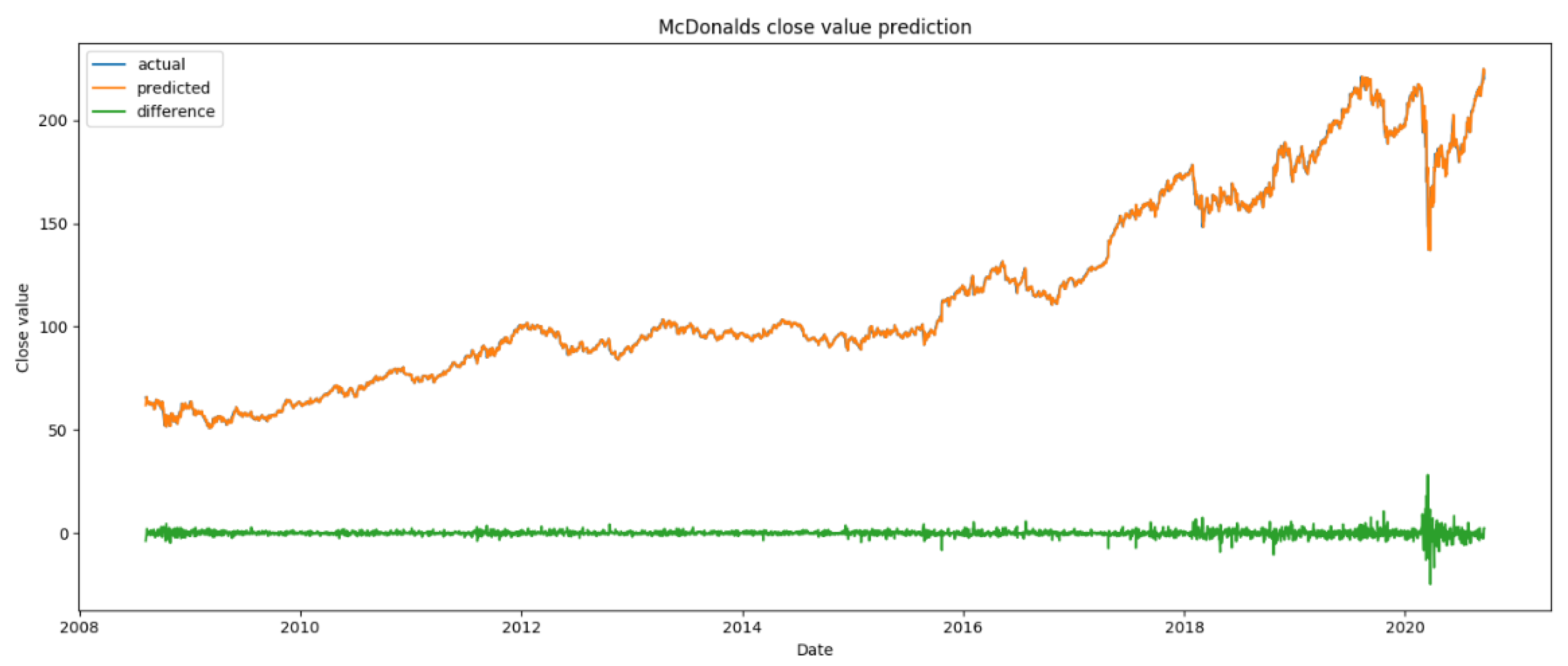
In the following graphics (Figure 3, Figure 4, Figure 5, Figure 6, Figure 7, Figure 8 and Figure 9), the predicted vs. actual values are displayed along the time axis. The algorithm kept a good performance, following the trends of market ‘close’ value through time, for all datasets. As expected, the algorithm suffered in its previsions around the time of the declared pandemic; however, it was able to achieve some stability afterwards, in line with the possible stability that the stock market can offer in such an unstable time.

It is also visible by the analysis of the graphics presented that although the value dropped significantly at the beginning of 2020, there is a trend of a continuous rise of the stock.

It is possible to infer that the algorithm learned the patterns quickly, making predictions that were very close to the actual ones with few data. The MAPE values were lower for every dataset in the more stable period before the pandemic, except for the McDonald’s and Visa datasets, which received better results in the total period. All MAPE values increased for the post-pandemic period, although not as much for the Amazon dataset—this can be explained by the more stable stock pricing in this company. In general, the RMSE and AAE values increased through time; since these are not percentage metrics, and the data are not normalized, this increase can be explained by the higher ‘close’ values in the stock market in the last few years across all datasets.

The results obtained in this experiment were very promising, showing that the HTM theory provides a solid framework for time series forecasting, achieving good predictions with few data. Furthermore, the algorithm maintained a good performance across the various datasets: through time, being robust to temporal noise, a bigger complexity of data, and a disruption in the input data caused by the pandemic.

Because of the way HTM works, it is hard to make a rigorous comparison with other methods, which normally divide datasets into training and testing batches.

Besides, in this study, the data used are specific to some S&P 500 companies, ranging from 3 January 2006 until 18 September 2020, contrary to what is observed in the literature, where the time range is typically smaller and no designation of the companies is made—although, some comparisons and findings can be discerned. In [13], the SMA network obtained a MAPE of 11.45% for only a short period of a year, a value worse than what was obtained in the present study for any company for the whole time period available on the datasets. The other two studies presented previously on Section 2, [12,14], related to the forecasting of the next day ‘close’ value using different LSTM networks, obtained better MAPE values. However, it cannot be stated that these networks perform better, since only a small percentage of the datasets are used for testing and rely on massive training sessions. These methods do not rely on an online continuous learning mechanism such as HTM.

6. Discussion and Conclusions

The advancements of how our brains work biologically may lead to new and revolutionary ways of achieving a true machine intelligence, the aim of the HTM theory. This theory should evolve through the years and help the science community to solve problems typically solved by Machine Learning; specifically Deep Learning in the last few years.

The proposed HTM network obtained good results in the time series forecasting of close values of the stock market, for seven different datasets, through time, proving it can be a great methodology to make predictions while being robust to noise in the data, both in a temporal and spatial axis. It is shown that the network can adapt to different datasets in the same range of problems, with no different hyper-parameter tuning, unlike LSTM and other Deep Learning models; this attribute of HTM models is linked to the known properties of the human cortical neurons and the representation of SDR. Another key difference from other Deep Learning models is that HTM learns continuously, without the need for a specific training dataset; the model learns and predicts continuously. The known experiments where the ‘close’ value of the stock market is predicted use a classic approach, where training/validation/test dataset tuning is applied to the comparison between models, which is difficult in terms of prediction accuracy; moreover, classically, the data are normalized and suffer a lot of data pre-processing, contrary to the HTM network, where the raw input is only transformed into an SDR, keeping its semantic characteristics.

7. Future Work

As the HTM theory develops, bringing new perspectives of the human intelligence and learning process, such as grid cells [26], it should grab more attention from the data science community, as it will provide a great framework for intelligence and learning.

With regards to future work, there are several possibilities that stand out:

• The combination of this theory with other methods of machine learning. In this way, high dimensional temporal learning problems requiring pre-processing and feature extraction can be solved before creating a sparse representation of the raw input;
• The application of this theory, or even the combination mentioned above, to the in-depth study of the impact of the pandemic on stock prediction;
• The extension of the application of this theory or combination to all S&P 500 companies and to other markets.

We believe that this approach has the most value, since not only does it prove that it is possible to obtain good results with HTM, but it also encourages future research and applications in this same field.