Time in Quantum Measurement

Abstract

Based on a model of quantum measurement we derive an estimate for the external measurement-time. Some interesting consequences will be analyzed.

1 Introduction

Given an apparatus or memory $\mathcal{A}$, a system $\mathcal{S}$ and the environment $\mathcal{E}$, the measurement process $\mathcal{M}$ can be represented by the following sequence:

(1)

The first step is the entanglement between the system $\mathcal{S}$ and the apparatus $\mathcal{A}$. The second step, d, is the decoherence of the entangled $\mathcal{AS}$ system by the perturbation through the environment $\mathcal{E}$ and the creation of classical alternatives. The third step, p, is the projection to one of the eigenstates and the record of a definite outcome. At this stage other states of the memory are being erased. In the course of this process the entropy of the $\mathcal{AS}$ system is going to fluctuate which reflects the expansion and compression of the abstract phase space spanned by the eigenvectors of a corresponding observable.

There is no algorithm (e.g differential equation) known to describe $\mathcal{M}$ exactly in time. The fluctuation of entropy alone makes it clear that the process $\mathcal{M}$ cannot be described in finite time by a Hamiltonian flow and the projection postulate does not refer to time at all. If we describe the decohered $\mathcal{AS}$ system by its density matrix ${\rho }_{\mathcal{AS}}$, there holds for the entropy $S_{{\rho }_{\mathcal{AS}}}=-tr{\rho }_{\mathcal{AS}}\log {\rho }_{\mathcal{AS}}\ge 0$. If the environment is supposed to be in thermal equilibrium of temperature T, the generalized Landauer principle [10] , [13] tells us that during the measurement process an amount of energy whose average over different measurement outcomes $\overline{E}$ satisfies

$$\overline{E}\ge kT{S}_{{\rho }_{\mathcal{AS}}},$$

(2)

is being dissipated.

2 Time

2.1 Dissipation

In the last paragraph we stated that the measurement process is accompanied by the dissipation of energy to the environment. So far no time parameter has entered the discussion. In the projection postulate quantum mechanics supposes that the realization of an eigenstate happenes instantaneously. The natural question arises whether the process $\mathcal{M}$ does not need some minimal amount of time to happen. Note that we are considering here the notion of external time [12] , i.e. the time valid outside the system $\mathcal{AS}$.

Let us rewrite sequence (1) for a representative model case where the apparatus $\mathcal{A}$, the system $\mathcal{S}$ and the environment $\mathcal{E}$ are one bit systems each and let $\psi ={\alpha }_1|1\rangle +{\alpha }_2|2\rangle$ be the measured state, A_i, i = 1, 2 the states of the apparatus and ε_i, i = 1, 2 the states of the environment. We may assume that $\langle 1|2\rangle =\langle A_0|A_1\rangle =\langle {\epsilon }_0|{\epsilon }_1\rangle =0$. Let $\mathcal{E}$ be in thermal equilibrium of temperature T. For the simplicity of notation we will just write down the coefficients ${\alpha }_i=\mathbb{C}$ and their conjugates ${\alpha }_i^{*}\in \mathbb{C},i=1,2$ of the density matrix and omit the basis vectors in each step of sequence (1). This leaves us with

In step d and p a total entropy of ${\overline{S}}^d+{\overline{S}}^p={\displaystyle \sum _{i=1,2}}{\left|{\alpha }_i\right|}^2\Delta S_i+k{\displaystyle \sum _{i=1,2}}{\left|{\alpha }_i\right|}^2\ln {\left|{\alpha }_i\right|}^2$ is being generated. By the second law of thermodynamics there must hold for the corresponding energies ${\overline{E}}^d+{\overline{E}}^p=T{\displaystyle \sum _{i=1,2}}{\left|{\alpha }_i\right|}^2\Delta S_i+kT{\displaystyle \sum _{i=1,2}}{\left|{\alpha }_i\right|}^2\ln {\left|{\alpha }_i\right|}^2\ge 0$, which is (2) [10] .

Note that to each outcome there corresponds an energy E_i, i = 1, 2.

2.2 External Time

2.2.1 Scope

In the sequel we would like to look at the question of minimal measurement time from an intrinsic angle. By intrinsic we mean that we abstract from a conscious observer. We solely base on elements given by our model, namely on the system $\mathcal{AS}$, the environment $\mathcal{E}$, the sequence (1) and the corresponding physical consequences (2). For the sequence (1) the word "realization" would probably be more accurate than "measurement" in this context. The projection and registering of the definite outcome with the necessary erasure of other/former states of the memory is an integral part of this measurement process. The information gained by decoherence has to be offset.

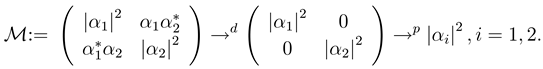
The connection between the environement $\mathcal{E}$ and the system $\mathcal{AS}$ which, from the intrinsic perspective of $\mathcal{E}$, gives proof of the definite outcome of $\mathcal{M}$, is only the dissipated energy. In first order approximation the dissipation can be described by some Hamiltonian $H_{\mathcal{ASE}}$ which is in our intrinsic sense unknown to the detector. 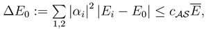In this situation we can apply the time-energy inequality [1]. Let us assume that the true energy is E_O. Following [1] , the intrinsic energy uncertainty on the basis of quantities given in our model is

(3)

where $c_{\mathcal{AS}}$ > 0 depends upon the system $\mathcal{AS}$.

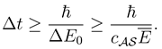
By the time-energy inequality [1] and (3) there holds for the lower bound on Δt

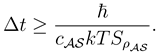
The lower bound holding for all possible measurements is therefore by (2)

(4)

This result can be interpreted that the process $\mathcal{M}$ takes, from the perspective of a generic detector in the environment $\mathcal{E}$, minimally a time interval $\Delta t=\frac{ħ}{c_{\mathcal{AS}}kT{S}_{{\rho }_{\mathcal{AS}}}}$ to happen.

2.2.2 Application

Let us assume that in empty Euclidean space there is a free particle, represented by a wave packet $\varphi \left(t\right)\in L^2\left({\mathbb{R}}^3\right)$ with fairly well defined momentum. Since its momentum is well known, by the Heisenberg uncertainty relation, its position is highly unprecise in ${\mathbb{R}}^3$. Classical theory, however, would say that this particle moves with constant velocity v along a straight line in the direction of the momentum vector. There is no way, given the uncertainty principle, to reconstruct directly the concept of classical trajectory and hence velocity defined by $v=\frac{\Delta x}{\Delta t}$ in the quantum realm.

By the help of our model, however, we will define a quantitiy which can be interpreted as the time Δt the particle needs to "reach" a point at distance R. This way we will come close to a reconstruction of classical velocity $v=\frac{R}{\Delta t}$.

We will use some technical facts: 1) −c ≤ x ln x ≤ x² for some fixed $c\in \mathbb{R}$ and all x ≥ 0, 2) L⁴(${\mathbb{R}}^3$) ⊂ L²(${\mathbb{R}}^3$), 3) lim_x→0 x^s ln x → 0, s, x > 0.

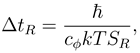
Let there be a free particle, φ(x) ≡ φ(r), in an environment which is in thermal equilibrium of temperature T. According to our model, the minimal time Δt_R needed to measure our particle at a distance of at least R would by (4) be

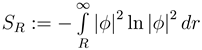
where S_R is defined as

(5)

and c_φ > 0 denotes the constant depending upon the set up (3).

The intuitive interpretation of Δt_R is the minimal time it takes for the particle to "reach" a point at distance R or further.

Note that, since S_R → 0 as R → ∞, the intuitive fact that it takes longer to reach more distant regions, is assured.

Next we want to better understand the dependency of S_R from R. Since φ ∈ L²(ℝ³) we have for some R₀ > 0, ε > 0

By the technical facts we have for any s ∈ ℝ, s > 0

If we set $s=\frac{1}{2}$, we get for R > R₀ big enough

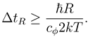
If we put the last result into the expression for time we get for R > 0 big enough

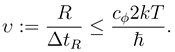
We now can define the analouge of classical velocity by

(6)

(6) gives us an upper bound which is independent of the distance R, for R big enough.

Interpretation We try to reconstruct as closely as possible an analogue of classical velocity from quantum mechanics. Thereby we focus on the reconstruction of the most simple situation where there is a free particle in space of temperature T. Due to the probabilistic nature of quantum mechanics it is clear that the reconstruction can only be done by using quantities which are at most analogous to the classical notions of "distance passed on a straight line" and "time to pass through that distance" which form the definition of classical velocity.

For the analogue of a classical particle moving on a straight line we use the radial symmetry of a free wave packet with fairly well defined momentum. Our model gives an estimate for the minimal time it takes to measure the position of this particle at a distance bigger or equal to R. It turns out that, if R is big enough, we find an estimate for the minimal time needed which is proportionate to the distance R, exactly what we would expect in the classical case. Note also that if R is big the value of the integral (5) is concentrated in an annulus around R. So the probability that the particle is detected outside an annulus [R, R + δ] , δ > 0 gets smaller as R gets bigger. We then interpret this time as the minimal time needed for our particle φ to "reach" a distance R and can reconstruct classical velocity. The fact that classically the particle moves with constant velocity is mirrored by an upper bound for the reconstructed velocity.

Note that estimate (6) can certainly be refined and is probably not the best estimate possible. If we could find an upper bound for c_ϕ , (6) would give a general bound on the velocity of a free particle.

3 Comments

Our ideas open some interesting perspectives on the philosophy of time. If conscious observers develop mathematical models of reality they carve out the systems under consideration and base their models on known energy functions or operators. Hence they do necessarily not account for the continuous interaction with the environement and the corresponding fluctuations of entropy. At the same time they are able to measure energies within arbitrarily short periods of time [1]. Consequently they conclude that time is a) reversible and b) continuous. Our intrinsic model tries to abstract as much as possible from the meta standpoint of a conscious observer and under these circumstances measurement, as defined in our model, needs some interval of time. Furthermore the measurement process is irreversible and could be a true source for the arrow of time.