Abstract
This paper describes a group-theoretic method for decomposing the entropy of a finite ensemble when symmetry considerations are of interest. The cases in which the elements in the ensemble are indexed by {1, 2, ..., n} and by the permutations of a finite set are considered in detail and interpreted as particular cases of ensembles with elements indexed by a set subject to the actions of a finite group. Decompositions for the entropy in binary ensembles and in ensembles indexed by short DNA words are discussed. Graphical descriptions of the decompositions of the entropy in geological samples are illustrated. The decompositions derived in the present cases follow from a systematic data analytic tool to study entropy data in the presence of symmetry considerations.
1 Introduction
The entropy H = − ∑j pj log pj of a finite set of n mutually exclusive events with corresponding probabilities p1,..., pn measures the amount of uncertainty associated with those events [1, p.3]. Its value is zero when any of the events is certain, it is positive otherwise, and attains its maximum value (log n) when the events are equally like, that is, p1 = ... = pn = 1/n. Alternatively [2, p.7], H is the mean value of the quantities − log pj and can be interpreted as the mean information in an observation obtained to ascertain the mutually exclusive and exhaustive (hypotheses defined by those) events.
In general, the probabilities of an ensemble with n elements are indexed by the set
and commonly indicated by p1, p2,..., pn. However, there are applications in which the elements in the ensemble exhibit intrinsic symmetries. Consider, for example, an election in which voters select their ordered preferences among the candidates in the list {a, b, c} by choosing one of the 6 permutations in the set
The resulting distribution
of relative frequencies of those choices is then an example of empirical probabilities indexed by permutations. Accordingly, the corresponding entropy is written as
In another example, the experimental results might be the empirical probabilities
with which the 16 binary sequences
in the DNA alphabet {A, G, C, T} appear in a given reference sequence of interest. Similarly, then, these probabilities are indexed by a set of labels structurally more interesting than {1, 2, ..., n}. In fact, the 16 binary words can be classified, for example, by permutations shuffling the letters in the DNA alphabet, or distinctly, by permutations shuffling the positions of those letters.
V = {1, ..., n},
V = {abc, cab, bca, bac, cba, acb}.
p′ = (pabc, pcab, ..., pacb)
p′ = (pAA, pAG, ..., pTT)
V = {AA, AG, ..., TT}
The objective of this paper is demonstrating that there is a systematic relationship among the labels, the (frequency) data indexed by those labels and the symmetries that are consistent with them, and showing that the methodology describing such relationship leads to the statistical analysis of the observed entropy of those frequency distributions.
The basic elements of symmetry studies are introduced in the next section and applied to the derivation of the standard (Section 3) and regular (Section 4) decompositions of entropy. In Section 5 a symmetry study of the entropy in Sloan Charts used in the quantification of visual acuity is presented. Additional comments are included in Section 6. The algebraic aspects present in this paper follow from the elements of the theory of linear representations of finite groups and can be found, for example, in [3, pp.1-24].
2 Symmetry Studies
The voting and the molecular biology data mentioned in the Introduction are examples of struc- tured data in symmetry studies [4,5]. These studies are centered on the notion of data (x) that are indexed by a finite set V of indices or labels (s) upon which certain symmetry transformations can be defined. Briefly, symmetry studies explore the symmetry transformations identified by the set of labels to facilitate the classification, interpretation and statistical analysis of the data {x(s), s ∈ V} indexed by these labels. A finite group (G) with g elements acts on V and determines a linear representation (ρ) of G that operates in the data vector space (). The resulting factor- ization of into a direct sum of invariant subspaces follows from the construction of algebraically orthogonal projections of the form = n ∑τ∈G χ(τ−1)ρ(τ)/g, one for each irreducible represen-tation (in dimension of n and character χ) of G. The canonical projections are the key elements leading to the explicit calculation and interpretation of the canonical invariants1x, 2x, ... in the data. If G has h irreducible representations, then there are h projections, and the identity operator I in reduces according to the sum I = 1 + 2 + .. . + h of algebraically orthogonal (ij = ji = 0 for i ≠ j) projection (i2 = i, i = 1, ..., h) matrices. A formal connection with the data analytical component of any symmetry study follows from the observation that basic decompositions of the form
for any inner product (·|·) defined in , can then always be studied within the context of statistical inference for quadratic forms [6,7]. As a consequence, symmetry-related hypotheses defined by the canonical invariants can be identified and assessed [8,9,10].
(x|y) = (x|1y) + (x|2y) + ... + (x|hy),
The present paper concentrates on two basic types of canonical decompositions. In the standard case the components of the probability distributions p′ = (p1, ..., pn) are indexed by the set V = {1, ..., n}, the symmetry transformations are defined by the group Sn of all permutations of those indices, which then acts on V according to
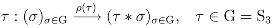
In the regularcase the components (pσ) of the probability distributions are indexed by the elements σ of a finite group (G, ∗) acting on itself according to
In closing this section it is opportune to remark that applications of group-theoretic principles in statistics and probability have a long history and tradition of their own, from Legendre-Gauss’s least squares principle through R.A Fisher’s method of variance decomposition. According to E.J. Hannan [11], the work [12] of A. James appears to be among the first describing the group- theoretic nature of Fisher’s argument, giving meaning to the notion of relationship algebra of an experimental design. In that same early period, U. Grenander [13] showed the effectiveness of harmonic analysis techniques to extend classical limit theorems to algebraic structures such as locally compact groups, Banach spaces and topological algebras. Two decades later, the relevance of group invariance and group representation arguments in statistical inference would become evident [14,15,16,17,18,19]. The integral of Haar, object of L. Nachbin’s 1965 monograph [20], became a familiar tool among statisticians. The work of S. Andersson on invariant normal models [21] is now recognized as a landmark concept extending and setting definitive boundaries to multivariate statistical analysis [22] in the tradition of T.W. Anderson. The collection of contemporary work in [23] clearly documents the present-day interest on those methods.
τ : (1, 2, ..., n) → (τ 1, τ 2, ..., τ n), τ ∈ Sn.
τ : (σ)σ∈G → (τ ∗ σ)σ∈G, τ ∈ G.
3 The Standard Decomposition of Entropy
Consider first a probability distribution p indexed by the set V = {1, 2}, that is p′ = (p1, p2). The group of permutations is S2 = {1, t}, where 1 indicates the identity and t indicates the transposition (12). S2 acts on V by permutation of the indices of their elements and the resulting linear representation
is given by
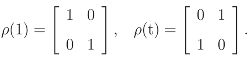 Note that ρ(τ) is the matrix defined by the change of basis {e1, e2} → {eτ1, eτ2} in the data vector space ℝ2. The canonical projections associated with ρ are defined by
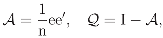
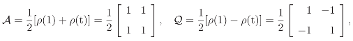 where the coefficients {1, 1} and {1, −1}determining 𝒜 and are the two irreducible characters of S2. Note that
and
where the coefficients {1, 1} and {1, −1}determining 𝒜 and are the two irreducible characters of S2. Note that
and
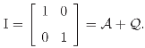 Let ℓ′ = (log(p1), log(p2)), so that H = −p′ℓ is the entropy in the probability distribution p. It then follows from I = 𝒜 + that H decomposes as
the components of which can be expressed as the log geometric mean
of the components of p, and as
Let ℓ′ = (log(p1), log(p2)), so that H = −p′ℓ is the entropy in the probability distribution p. It then follows from I = 𝒜 + that H decomposes as
the components of which can be expressed as the log geometric mean
of the components of p, and as
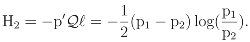 Because H2 can be expressed as
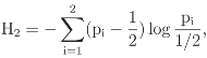 it then follows that −H2 is precisely Kullback’s [2, p.110] divergence between p and the uniform distribution e′/2 = (1, 1)/2, thus justifying the interpretation of entropy as a measure of non- uniformity.
𝒜 = 𝒜 = 0, 𝒜2 = 𝒜, 2 = ,
H = −p′ℓ = −p′Iℓ = −(p′𝒜ℓ + p′ℓ),
H1 = −p′𝒜ℓ= −  log(p1p2)
log(p1p2)
The standard decomposition of the entropy obtained for two-component distributions extends to n−component distributions in the expected way. Writing
 where ee′ is the n × n matrix of ones, it then follows that the canonical decomposition is exactly
Clearly, it satisfies 𝒜2 = 𝒜, 2 = and 𝒜 = 𝒜 = 0. Moreover, 𝒜 projects = ℝn into a subspace a of dimension tr 𝒜 = 1 generated by e = e1 + .. . + en = (1, 1, ..., 1)′ ∈, whereas projects into an irreducible subspace q in dimension tr = n − 1, the orthogonal complement of a in . The irreducibility of q, proved using character theory [3, p.17; 5, p.70], shows that the reduction = a + q is exactly the canonical reduction determined by ρ. This decomposition is referred to as the standard decomposition or reduction. Applying the standard reduction I = 𝒜 + to the entropy H = −p′ℓ of a distribution p′= (p1, ..., pn), where ℓ′ = (log(p1), ..., log(pn)), it follows, in summary,
where ee′ is the n × n matrix of ones, it then follows that the canonical decomposition is exactly
Clearly, it satisfies 𝒜2 = 𝒜, 2 = and 𝒜 = 𝒜 = 0. Moreover, 𝒜 projects = ℝn into a subspace a of dimension tr 𝒜 = 1 generated by e = e1 + .. . + en = (1, 1, ..., 1)′ ∈, whereas projects into an irreducible subspace q in dimension tr = n − 1, the orthogonal complement of a in . The irreducibility of q, proved using character theory [3, p.17; 5, p.70], shows that the reduction = a + q is exactly the canonical reduction determined by ρ. This decomposition is referred to as the standard decomposition or reduction. Applying the standard reduction I = 𝒜 + to the entropy H = −p′ℓ of a distribution p′= (p1, ..., pn), where ℓ′ = (log(p1), ..., log(pn)), it follows, in summary,
 between p and the uniform distribution e′/n. This can be easily verified by direct evaluation of the RHS of the above equality.
I = 𝒜 + .
Proposition 3.1
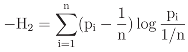
Similarly to the case n = 2 described earlier, (−1×) the entropy of a n−component distribution decomposes as the sum of the log geometric mean and Kullback’s divergence
The standard reduction of the entropy H in p′ = (p1, ..., pn) is H = H1 + H2 with
3.1 Graphical displays of {H1, H2}
It is observed that both H1 and H2 remain invariant under Sn, in the sense that for = 𝒜, ,
The last equality in (3.1) is a consequence of the fact that and ρ(τ) commute for all τ ∈ Sn. Therefore, H1 and H2 define a set of one-dimensional invariants that can be jointly displayed and interpreted, along with any additional covariates. Graphical displays such as these are generically called invariant plots.
(ρ(τ)p)′(ρ(τ)ℓ) = p′ρ(τ)′ρ(τ)ℓ = p′ℓ.
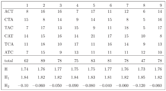
Table (3.3) shows the observed frequencies with which the words in the permutation orbit
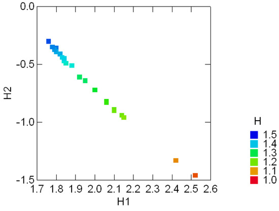
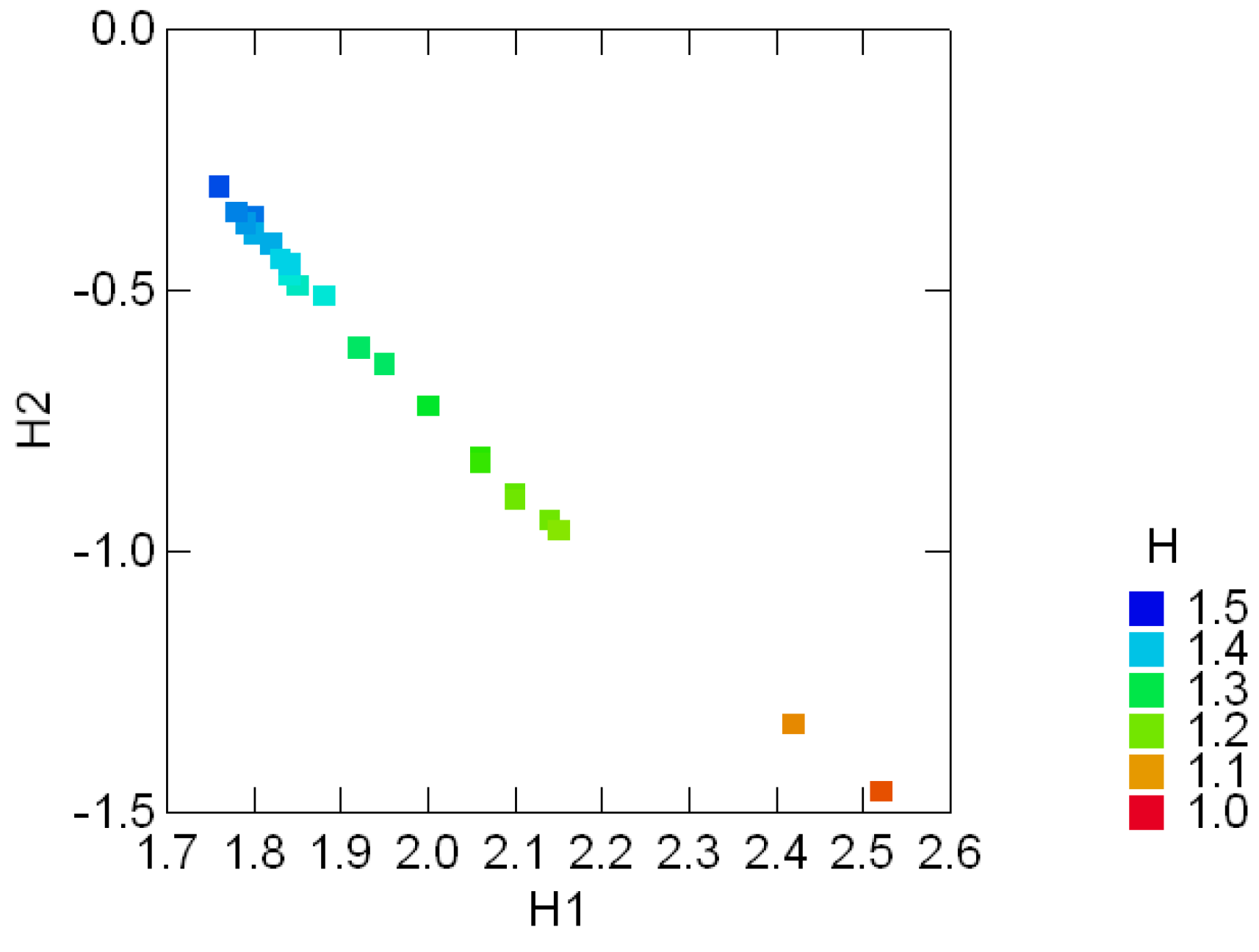
of the DNA word ACT appear in 9 subsequent regions of the BRU isolate K02013 of the Human Immunodeficiency Virus Type I. To locate the sequence in the National Center for Biotechnology Information (http://www.ncbi.nlm.nih.gov) data base, use the accession number K02013. Each region is in length of 900 base pairs. Table (3.3) also shows the entropy (H) of each distribution and its standard decomposition: the log geometric mean (−H1) and divergence (−H2) relative to the uniform distribution e′/6. In the present example S6 acts on V by permutation of the six DNA words. In the next section the same frequency data will be studied under the permutation action of S3 on the letters of the DNA words.
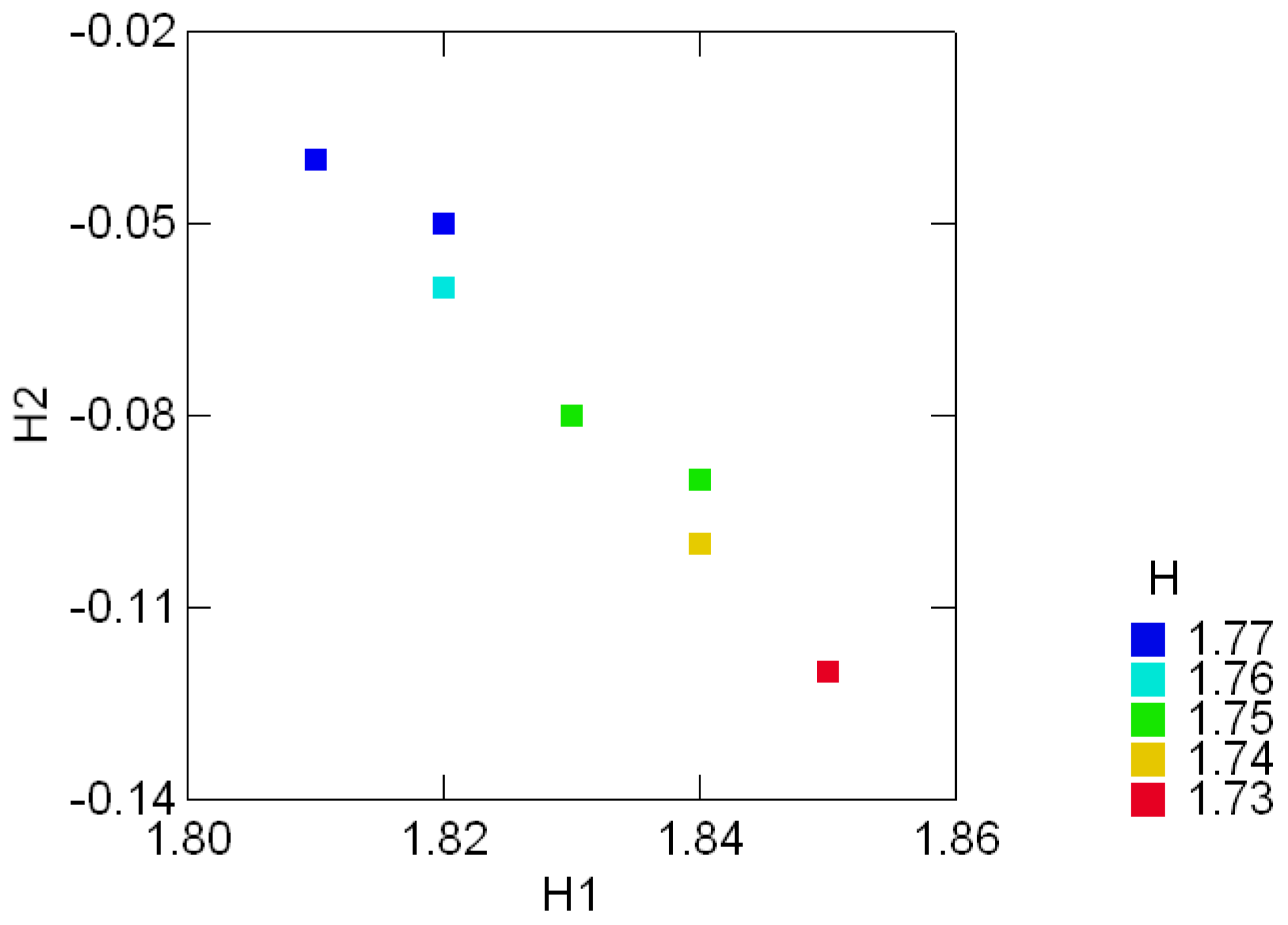
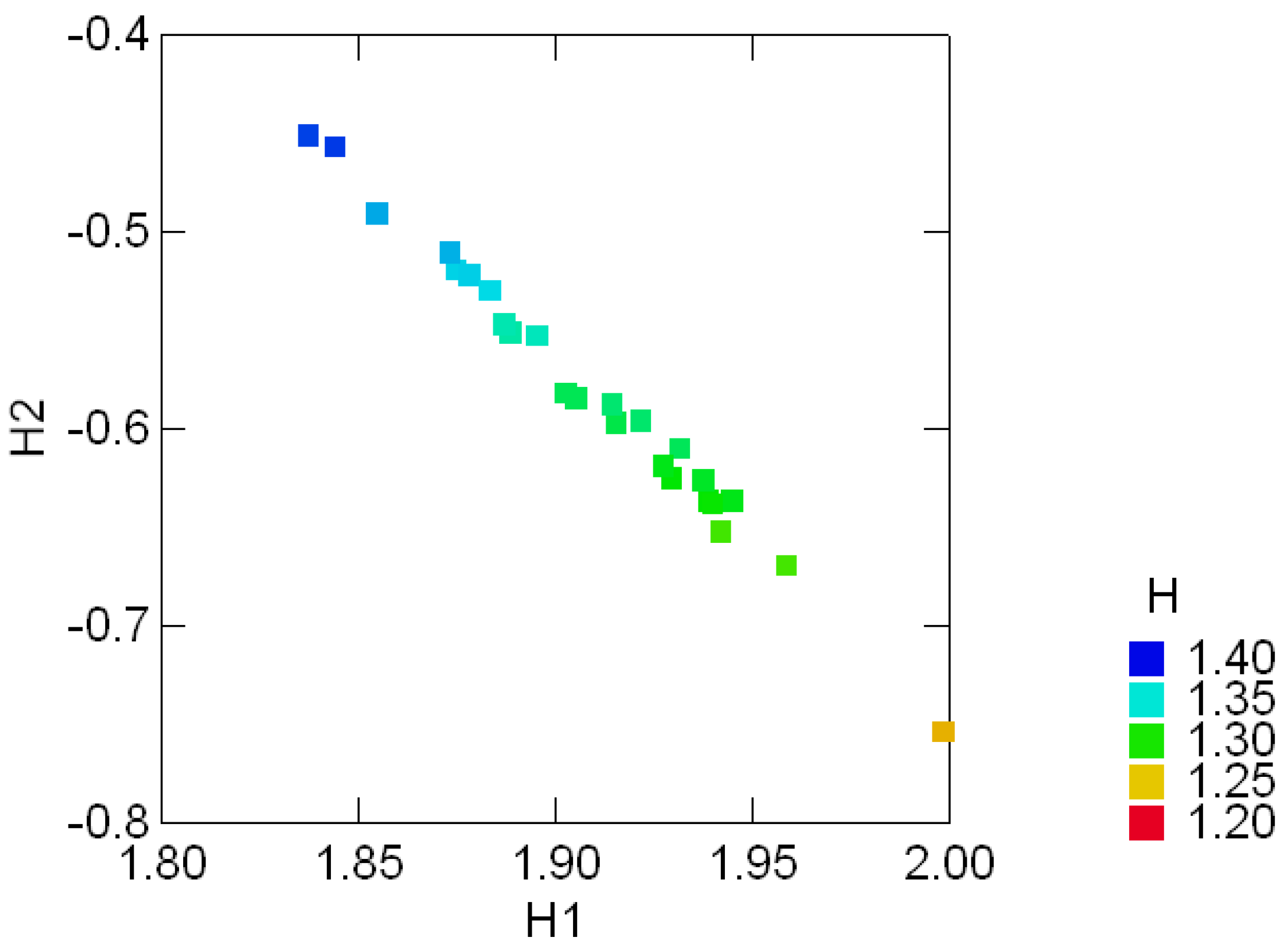
 The invariant plot of Figure 3.1 shows the (color coded) entropy of the ACT orbit and its invariant components (H1, H2) in each one of nine regions. Note, for example, that the entropy in regions 3 and 6 are equal and yet their location in the invariant plot differ, showing a slightly increased divergence from the uniform distribution e′/6 in region 3. Although the entropy in regions 6 and 8 is essentially the same, there is a three-fold ratio between their divergence components- this is noticeable by inspecting the (lack of) uniformity in the corresponding frequency distributions. Differentiations of that nature are possible because the dimension of the invariant subspace asso- ciated with H2 is tr = n − 1, where n is the number of components in the distribution under consideration. The regular decomposition described in the next section will further illustrate these differentiations and their relation to the symmetries imposed in the set of labels for the components of the distributions.
V = {ACT, CTA, TAC, CAT, TCA, ATC}
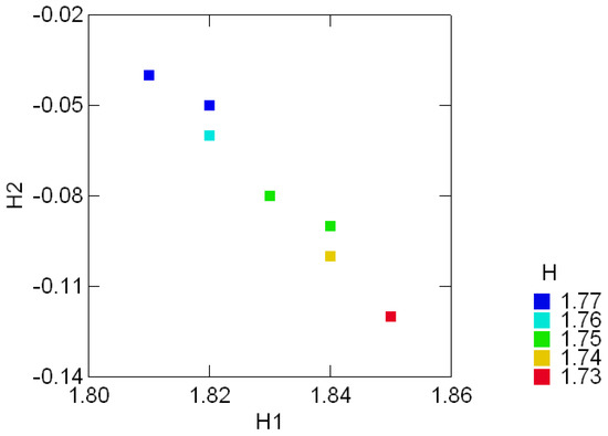
Figure 3.1:.
Color coded entropy levels (H) and their invariant components {H1, H2} in 9 subsequent regions of the HIV virus Type I (BRU isolate).
Figure 3.1:.
Color coded entropy levels (H) and their invariant components {H1, H2} in 9 subsequent regions of the HIV virus Type I (BRU isolate).
3.2 The standard decomposition of the entropy of the Sloan fonts
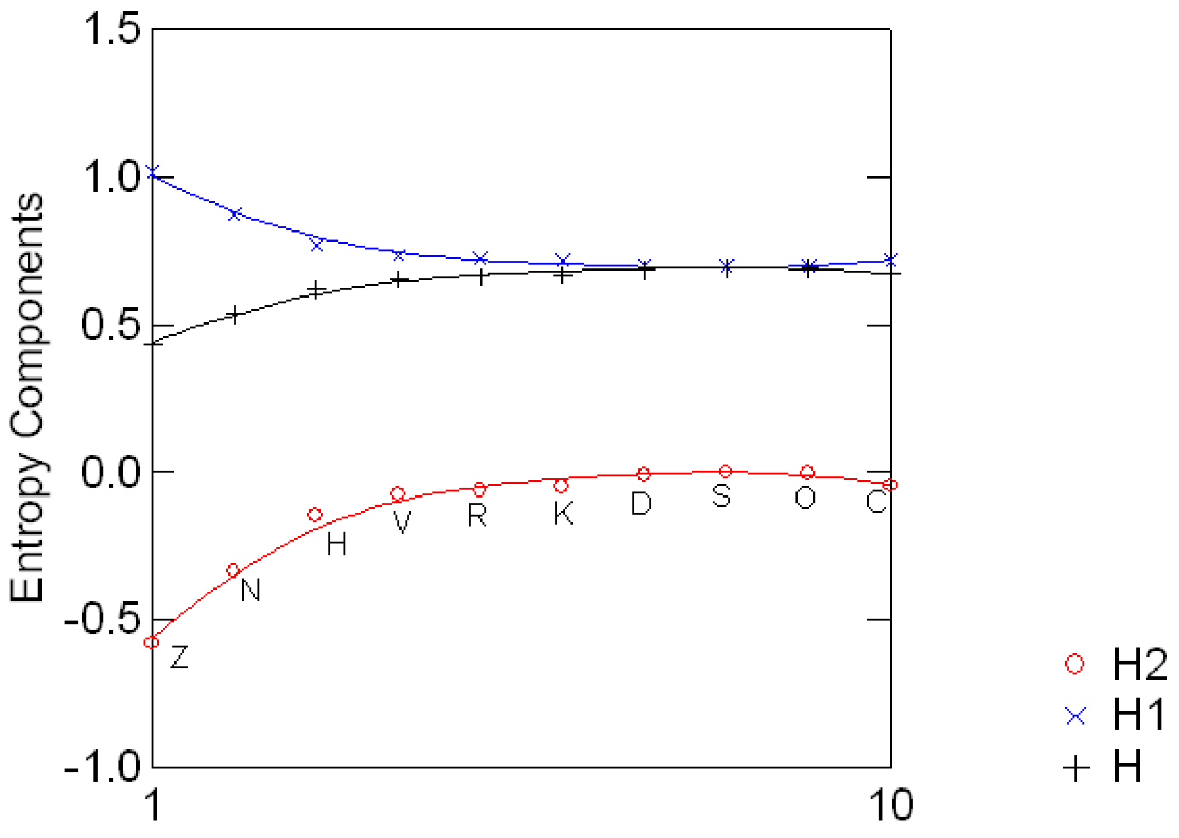
Table (3.4) shows the ten Sloan fonts [24, Table 5] used for the assessment of visual acuity in the Early Treatment Diabetic Retinopathy Study, along with their estimated difficulty (probability of incorrectly identifying the letter), the corresponding entropy and their standard invariant compo- nents H1 and H2. Figure 3.2 shows the standard decomposition for each letter. The divergence from the uniform distribution e′/2 ranges from 0.58 when the distribution is (0.844, 0.156) to 0.001 for (0.516, 0.484). The study of the entropy of Sloan fonts will continue later on in Section 5.
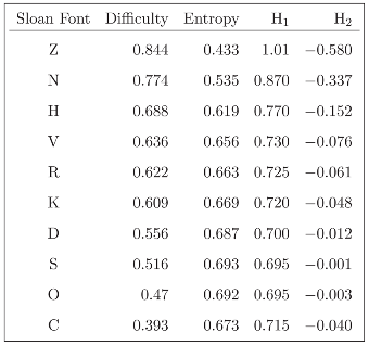
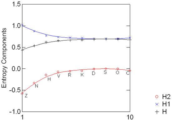
Figure 3.2:.
Entropy canonical components for the ten Sloan fonts.
Figure 3.2:.
Entropy canonical components for the ten Sloan fonts.
3.3 Geological compositions
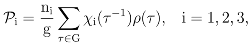
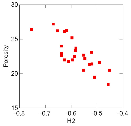
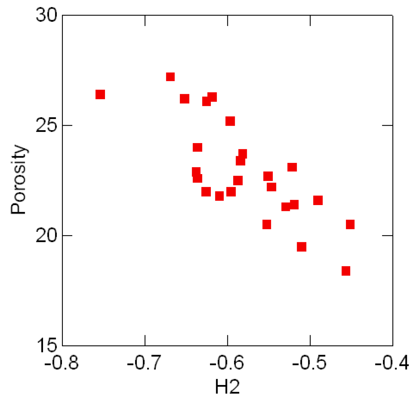
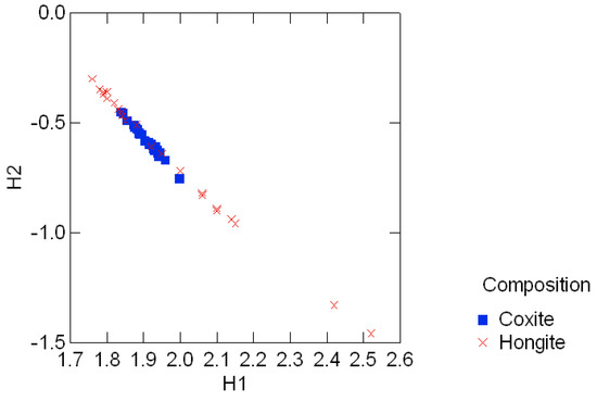
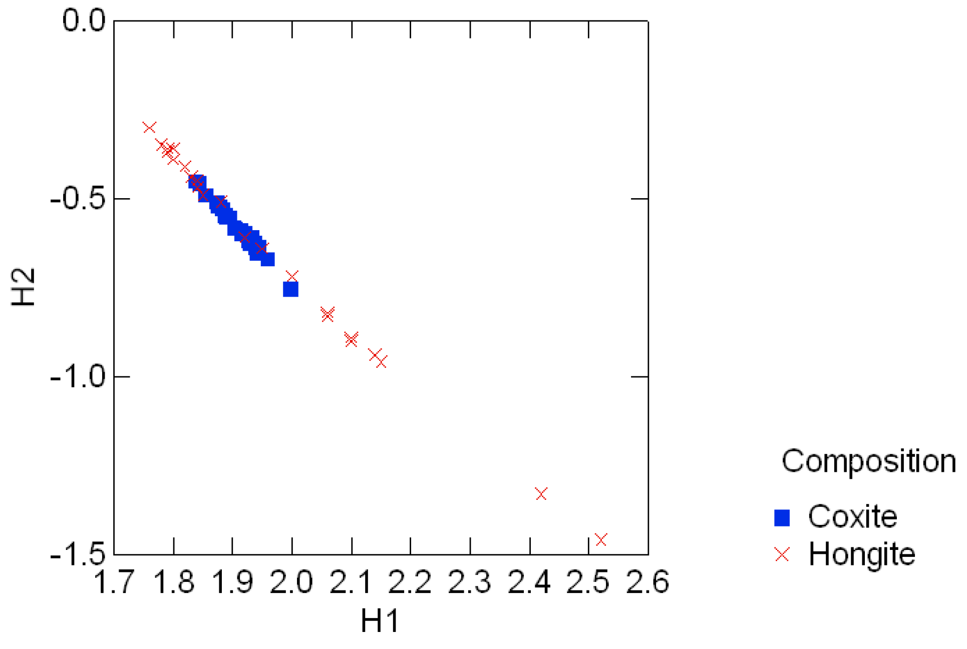
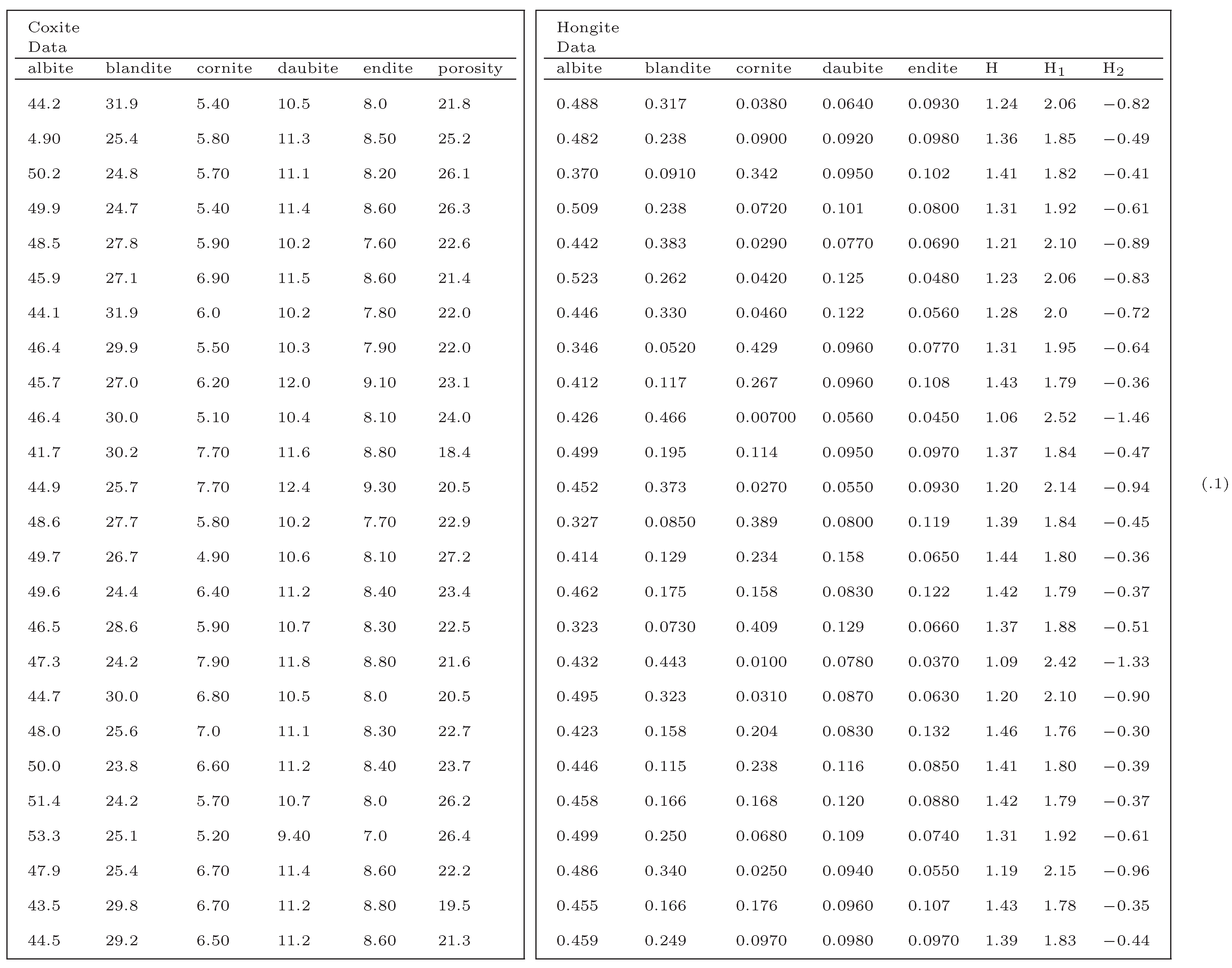
Tables .1 in Appendix A appear in [25, pp. 354, 358] and show the geological compositions of albite, blandite, cornite, daubite and endite in 25 samples of coxite and hongite, in addition to the porosity (percentage of void space) of each sample of coxite. In this example, probability distributions are referred to as compositions, following [25, p.26]. Figure 3.3 and Figure 3.4 show, re- spectively, the color coded entropy and porosity levels for the coxite samples, and their invariant components {H1, H2}. The entropy among all compositions is within the range of 75 − 87 percent of the max entropy (log 5 = 1.6), thus being concentrated in a relatively narrow region. The joint distribution of porosity and H2 shown in Figure 3.5 suggests that porosity is negatively correlated with H2, or, equivalently, positively correlated with the divergence. In fact, the observed sample correlation coefficient based on 25 samples of these two variables is 0.78.
Figure 3.6 shows the color coded entropy in the hongite samples and their invariant components {H1, H2}. Figure 3.7 clearly shows the contrasting difference in entropy range between the two minerals, also evident in the range of the divergence in those compositions. This noticeable feature of the compositions [25, p.4], namely that coxite compositions are much less variable than hongite compositions, is clearly captured in these invariant plots.
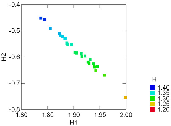
Figure 3.3:.
Color coded entropy levels (H) and their invariant {H1, H2} components in the geo-logical compositions of 25 samples of coxite.
Figure 3.3:.
Color coded entropy levels (H) and their invariant {H1, H2} components in the geo-logical compositions of 25 samples of coxite.
4 Regular Decompositions of Entropy
In this section, the decomposition of the entropy for probability ensembles with components in- dexed by S3, the group of permutations of three objects, will be considered. Decompositions for ensembles indexed by other finite groups can be obtained similarly.
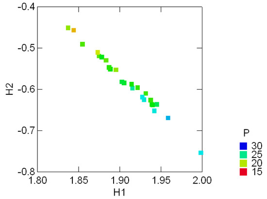
Figure 3.4:.
Color coded porosity levels (P) and their invariant entropy components {H1, H2} in the geological compositions of 25 samples of coxite.
Figure 3.4:.
Color coded porosity levels (P) and their invariant entropy components {H1, H2} in the geological compositions of 25 samples of coxite.

To illustrate, consider the DNA word ACT and its permutation orbit
introduced early on in Section 3.1. Note that V can be generated from the word ACT by applying, respectively, the permutations
 defining the group S3, so that V is isomorphic to S3. Indicate by
the respective relative frequencies with which the words in V, or equivalently, the elements in S3, appear in a given DNA reference region. These relative frequencies are, consequently, data indexed by S3. Let also ℓ indicate the vector of the log components of p, so that H = −p′ℓ is the entropy in the probability distribution p indexed by S3.
defining the group S3, so that V is isomorphic to S3. Indicate by
the respective relative frequencies with which the words in V, or equivalently, the elements in S3, appear in a given DNA reference region. These relative frequencies are, consequently, data indexed by S3. Let also ℓ indicate the vector of the log components of p, so that H = −p′ℓ is the entropy in the probability distribution p indexed by S3.
V = {ACT, CTA, TAC, CAT, TCA, ATC}
p′ = (r1, r2, r3, t1, t2, t3)
4.1 The regular decomposition
The permutations in S3 act on the DNA words by shuffling the letters. This gives a linear representation
 ρ of S3. Each matrix ρ(τ) is defined in the vector space for the data indexed by S3. Associated with ρ there are three canonical projections
 corresponding to the irreducible characters
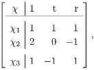 of S3, with n1 = n3 = 1, n2 = 2, g = 6, t = {(12), (13), (23)}, r = {(123), (132)}, given by
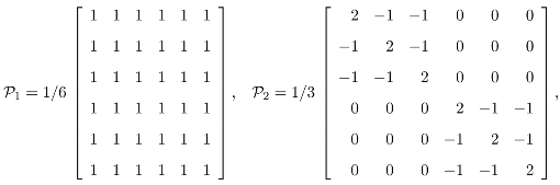 and
and
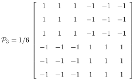
 Observe that ij = ji = 0 for i ≠ j,
  = i, i = 1, 2, 3 and I = 1 + 2 + 3. The underlying invariant image subspaces ix, x ∈ ℝ6, are in dimension of 1, 4, 1 respectively.
Figure 3.5:.
Porosity levels and divergence components H2 in 25 samples of coxite.
Figure 3.5:.
Porosity levels and divergence components H2 in 25 samples of coxite.
Figure 3.6:.
Color coded entropy levels (H) and their invariant {H1, H2} components in the geological compositions of 25 samples of hongite.
Figure 3.6:.
Color coded entropy levels (H) and their invariant {H1, H2} components in the geological compositions of 25 samples of hongite.
= i, i = 1, 2, 3 and I = 1 + 2 + 3. The underlying invariant image subspaces ix, x ∈ ℝ6, are in dimension of 1, 4, 1 respectively.It then follows that
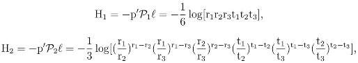
with the regular components of the entropy H given by
 and
and
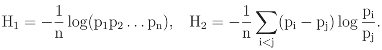
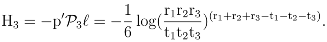 The interpretation of these components can be expressed in terms of three axial reflections (trans- positions) and the three-fold rotations (cyclic permutations) of the regular triangle: −H1 is the log geometric mean of the components of p; direct evaluation shows that
where r• is the marginal probability r1 + r2 + r3 of a rotation, t• is the marginal probability t1 + t2 + t3 of a reflection, D(r : u) is Kullback’s divergence between the rotation subcomposition [25, p.33]
The interpretation of these components can be expressed in terms of three axial reflections (trans- positions) and the three-fold rotations (cyclic permutations) of the regular triangle: −H1 is the log geometric mean of the components of p; direct evaluation shows that
where r• is the marginal probability r1 + r2 + r3 of a rotation, t• is the marginal probability t1 + t2 + t3 of a reflection, D(r : u) is Kullback’s divergence between the rotation subcomposition [25, p.33]
 and the uniform distribution u = e′/3, and D(t : u) is the divergence between the reflection subcomposition t = (t1, t2, t3)/(t1 + t2 + t3) and the uniform distribution u; and
 It is then possible to summarize the regular decomposition of the entropy of a distribution p in- dexed by S3 as a three-component sum: the log geometric mean of p, the total uniform divergence within rotations and within reflections and a component measuring the between rotations and reflections separation.
H = −p′ℓ = −p′1ℓ− p′2ℓ− p′3ℓ,
−H2 = r•D(r : u) + t•D(t : u)
r = (r1, r2, r3)/(r1 + r2 + r3)
Figure 3.7:.
Entropy levels in the standard invariant plot for coxite and hongite data.
Figure 3.7:.
Entropy levels in the standard invariant plot for coxite and hongite data.
Table (4.1) shows the regular decomposition H = H1 + H2 + H3 for the permutation orbit of ACT in each one of 9 adjacent regions of the isolate. Table (4.2) shows the ratios H1/H and H2/H3 for potential comparisons among these regions. Similar ratios were calculated for the words AGT and ACG (Tables (4.3) and (4.4), respectively). The regions 1 and 4 were removed from the calculations for ACG due to presence of zeros in the frequency distributions.
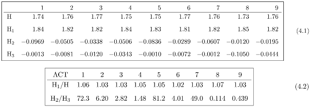
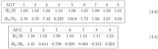 The within-region and between-words in the ratios of the entropy regular components for the three DNA words considered in this example is striking. In particular, the ratio H2/H3 clearly differentiates the ACG orbit from ACT and AGT. The between-region range of the ratios H2/H3 is 0.295 − 1.45 in the ACG orbits, in contrast to 0.222 − 108 in the AGT orbits and 0.114 − 72.3 in the ACT orbits.
5 A Symmetry Study of Sloan Charts
This study will combine the notions developed in the previous sections by introducing the Sloan Charts and considering each line in the chart as the sampling unit (total of 42 lines); identifying the group G of planar symmetries of the Sloan fonts; determining the invariants associated with the regular representation of G and studying the line entropy in that space. Cyclic permutation orbits have been used [26] to describe the evolutionary strategy of the HIV-1 virus.
5.1 The Sloan Charts and the Sloan Fonts symmetries
Tables (5.2) show a Sloan Chart [24, Table 5] developed for use in the Early Treatment Diabetic Retinopathy Study and the 10 individual Sloan letters appearing in Example 3.2, their symmetry transformations, the single-letter difficulty as the estimated [24] probability of incorrectly identi- fying the letter, and the corresponding entropy.
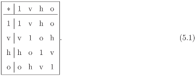
The group of interest here is the point planar group G = {1, o, v, h}, in which 1 is the identity, o the point symmetry or inversion, v the vertical axis reflection and h the horizontal axis reflection. The font is considered centered at the center of inversion with their natural vertical and horizontal directions along the corresponding axes of reflection. Observe that the symmetries indicated in the RHS Table in (5.2) are the subgroups of G leaving the letter fixed (or the letter stabilizer). G is an Abelian group isomorphic to C2 × C2 and its multiplication table is given by
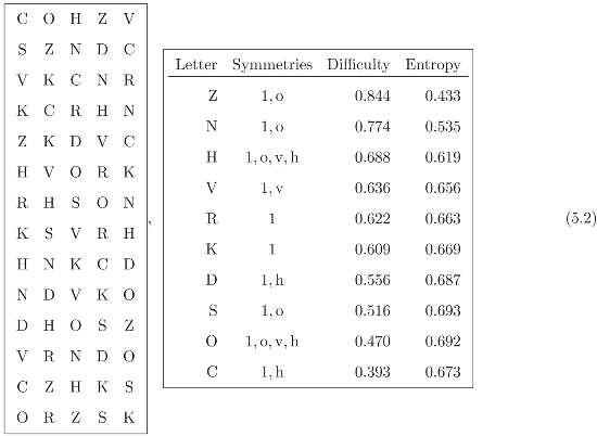 The objective here is studying the relationship between line entropy and letter symmetry based on 42 ETDRS lines, obtained from three charts similar to the one shown in the LHS table in (5.2).
5.2 The regular decomposition
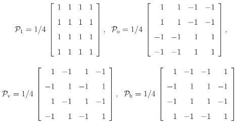
The canonical projections for the regular representation (G acting on itself) are given by
 Indicating, for simplicity of notation, by x′= (1, o, v, h) a generic vector of data indexed by G, direct evaluation shows that
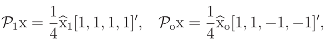
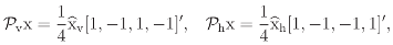 where
where  are the Fourier transforms
1 = 1 + o + v + h, o = 1 +o − v − h,
v = 1 + v − o − h, h = 1 + h − o − v,
evaluated at the irreducible one-dimensional representations of G.
are the Fourier transforms
1 = 1 + o + v + h, o = 1 +o − v − h,
v = 1 + v − o − h, h = 1 + h − o − v,
evaluated at the irreducible one-dimensional representations of G.
are the Fourier transforms
1 = 1 + o + v + h, o = 1 +o − v − h,
v = 1 + v − o − h, h = 1 + h − o − v,
Note, as shown in Appendix B, that
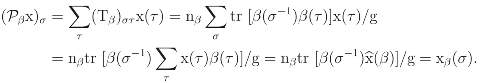
 that is, the entry x(τ) of the regular β-invariant βx is precisely xβ(τ) = nβtr [β(τ−1) (β)]/g. Consequently, the data assignment xβ identifies the properties of the regular canonical projection β with the properties of the Fourier transform (β) evaluated at β. In that sense, the indexing xβ should retain the interpretations associated with the invariant subspace of β, and, jointly, the data vectors {xβ, β ∈
  } should fully describe the regular symmetry invariants. Here indicates the set of all irreducible representations of G. Any indexing x of G decomposes (via the Fourier inverse formula) as the linear superposition ), ∑β∈ xβ(τ) of regular invariants xβ of G. Shortly, then x = ∑β∈ )xβ.
(β)]/g. Consequently, the data assignment xβ identifies the properties of the regular canonical projection β with the properties of the Fourier transform (β) evaluated at β. In that sense, the indexing xβ should retain the interpretations associated with the invariant subspace of β, and, jointly, the data vectors {xβ, β ∈ } should fully describe the regular symmetry invariants. Here indicates the set of all irreducible representations of G. Any indexing x of G decomposes (via the Fourier inverse formula) as the linear superposition ), ∑β∈ xβ(τ) of regular invariants xβ of G. Shortly, then x = ∑β∈ )xβ.5.3 Sorting the line entropy by font symmetry type
Indicate by
the set of elements in V that remain fixed by the symmetry transformation τ applied to s ∈ V according to the rule ϕ. Then there is a general method of indexing the data by G, called the regular indexing, constructed as follows: to each element τ ∈ G associate the evaluation x(τ) of a scalar summary of x defined over the set fix (τ). That is, x(τ) indicates a summary of the data over those elements (if any) in V that share the symmetry of τ . For example, if the summary of interest is the averaging, then
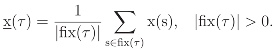 As an example, the regular indexing is applied to the font entropy data x(s) of each font s in each line (V) of the Sloan Chart shown in the LHS Table in (5.2). Here fix(τ) is the set of fonts with the symmetry of τ ∈ G, and x(τ) is the average font entropy over the set of fonts with the symmetry of τ , or the mean line entropy conditional to fonts with symmetry of τ . Table (5.3) shows the line entropy indexed, or sorted, by the symmetries of G. Note that line 2 was excluded because there were vertical symmetries in that line. One can then proceed with the study of the regular decomposition for x as data indexed by the group G of planar symmetries.
fix (τ) = {s ∈ V; ϕ(τ,s) = s} ⊆ V
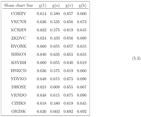
Figure 5.1 shows the line entropy distribution classified by font symmetry Eτ ≡ x(τ) over 39 Sloan
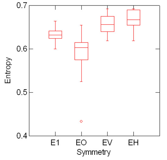
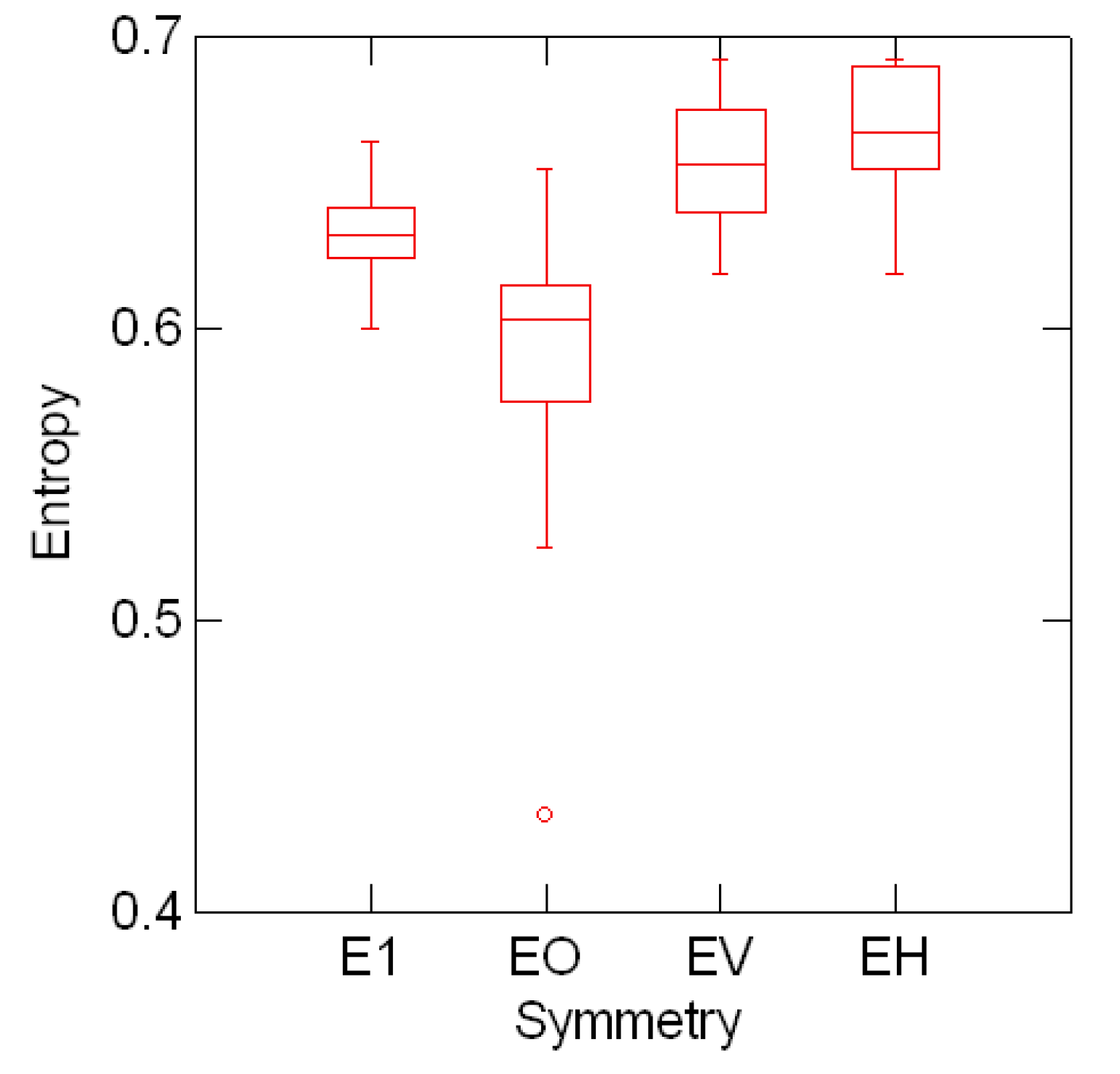 charts lines. In three of the 42 lines the frequency counts were not all positive and those lines were
 deleted. The results suggest a (statistically) significant drop in mean line entropy conditional to fonts with point symmetry. This result should be explored further taking into account, for example, the fact that the mean number of letters per line (± standard deviation) with point, horizontal and vertical symmetry are, respectively, 2.5 ± 0.804, 2.0 ± 0.698, and 1.5 ± 0.741.
Figure 5.1:.
Mean line entropy distribution and font symmetry Eτ ≡ x(τ).
Figure 5.1:.
Mean line entropy distribution and font symmetry Eτ ≡ x(τ).
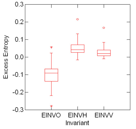
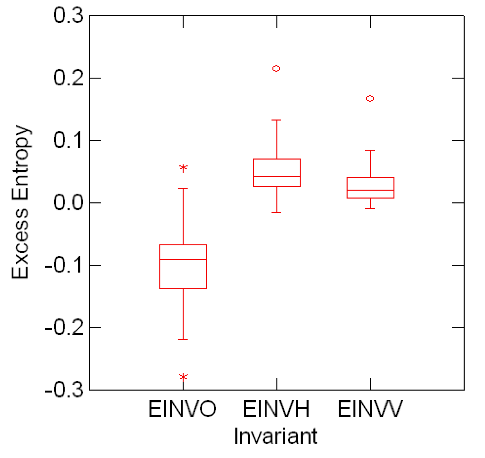
Figure 5.2:.
Distribution of the entropy invariants EINVO≡ o, EINVV ≡ v and EINVH≡ h for the entropy data indexed by font symmetries.
o, EINVV ≡ v and EINVH≡ h for the entropy data indexed by font symmetries.
Figure 5.2:.
Distribution of the entropy invariants EINVO≡ o, EINVV ≡ v and EINVH≡ h for the entropy data indexed by font symmetries.
o, EINVV ≡ v and EINVH≡ h for the entropy data indexed by font symmetries.In addition, Figure 5.2 shows the distribution of the Fourier transforms 2, 3 and 4 (second, third and fourth invariants) for the entropy data
of Table (5.3) indexed by the font symmetries. Consistently with the previous interpretation, the distribution of the invariant o is markedly shifted from the distributions of v and h.
2, 3 and 4 (second, third and fourth invariants) for the entropy data
{x(1), x(o), x(v), x(h)}
o is markedly shifted from the distributions of v and h.6 Summary and Comments
This paper introduced the standard decomposition H = H1 + H2 of the entropy of any finite distribution and the method for obtaining the regular decomposition H = H1 + .. . for the entropy of distributions indexed by arbitrary finite groups.
- The standard decomposition appears in analogy with the decomposition of the sum of squares, or, more specifically, to the decomposition of an inner product (y|x) of two vector x and y in the same finite-dimensional vector space. In fact, the standard decomposition I = 𝒜 + has a well-known role in statistics. It leads to the usual decompositionof the sum of squares in terms of the sample average and the sample variance
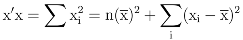
 . Similarly, it decomposes x’y into the sum
  ;
; - The methodology presented in this paper should provide an additional tool to study the entropy in distributions of nucleotide sequences in molecular biology data. This case is also of statistical and algebraic interest because it extends the decompositions introduced in the present paper to the case in which the probability distributions are indexed by the short nucleotide sequences upon which a group may act by symbol symmetry or by position symmetry [5, p.40];
- Two-dimensional invariant plots for the regular decomposition of the entropy by S3 can be obtained by jointly displaying the three pairwise combinations of the invariant components {H1, H2, H3}. The characteristic of the regions of constant entropy in these planes needs to be investigated;
- The large-sample theory for multinomial distributions, described in detail, for example, in [27, p.469], can be applied to derive the moments of the entropy components.
Appendix A
Appendix B
With the notation introduced in Section 5.2, define the g × g matrix
in which the rows and columns are indexed by the elements of G. Let also
 indicate be the regular canonical projection associated with β ∈ .
(Tβ)στ = nβtr [β(σ−1τ)]/g,
.Proposition B.1
β = Tβ.
Proof:
To see this, use the fact that the single unitary entry in row σ of φ(γ) is at column τ if and only if σ = γτ, or γ = στ−1, so that (β)στ = nβ χβ (στ−1M)/g = nβtr β(στ−1)/g = (Tβ)στ, as stated.
Moreover, because the Fourier transform (β) = ∑τ ∈G x(τ)β(τ) of the scalar function x is also an element in  , the indexing xβ(τ) = nβ tr [β(τ−1) (β)]/g is well-defined. The following proposition shows that it reduces as β.
(β) = ∑τ ∈G x(τ)β(τ) of the scalar function x is also an element in , the indexing xβ(τ) = nβ tr [β(τ−1) (β)]/g is well-defined. The following proposition shows that it reduces as β.Proposition B.2
xβ(τ) = nβtr [β(τ−1) (β)]/g is an invariant of β.
(β)]/g is an invariant of β.Proof:
Using the identity β = Tβ derived above, for an arbitrary vector x ∈ ℝg, it follows that
 That is, the entry x(τ) of the regular β-invariant βx is precisely xτ(τ) = nβtr [β(τ−1) (β)]/g.
(β)]/g.Acknowledgments
The author is thankful to the referees and the editor for their judicious comments and insightful suggestions.
References
- Khinchin, A. I. Information theory; Dover: New York, NY, 1957. [Google Scholar]
- Kullback, S. Information theory and statistics; Dover: New York, NY, 1968. [Google Scholar]
- Jean-Pierre Serre. Linear representations of finite groups; Springer-Verlag: New York, 1977. [Google Scholar]
- Viana, M. Symmetry studies- an introduction; IMPA Institute for Pure and Applied Mathematics Press: Rio de Janeiro, Brazil, 2003. [Google Scholar]
- ——, Lecture notes on symmetry studies, Technical Report 2005-027, EURANDOM, Eindhoven University of Technology, Eindhoven, The Netherlands. 2005. Electronic version http://www.eurandom.tue.nl.
- Eaton, M. L. Multivariate statistics- a vector space approach; Wiley: New York, NY, 1983. [Google Scholar]
- Muirhead, R. J. Aspects of multivariate statistical theory; Wiley: New York, 1982. [Google Scholar]
- Lakshminarayanan, V.; Viana, M. Dihedral representations and statistical geometric optics I: Spherocylindrical lenses. J. Optical Society of America A 2005, 22, no. 11. 2843–89. [Google Scholar]
- Viana, M. Invariance conditions for random curvature models. Methodology and Computing in Applied Probability 2003, 5, 439–453. [Google Scholar]
- Viana, M.; Lakshminarayanan, V. Dihedral representations and statistical geometric optics II: Elementary instruments. J. Modern Optics To appear. 2006. [Google Scholar]
- Hannan, E. J. Group representations and applied probability. Journal of Applied Probability 1965, 2, 1–68. [Google Scholar]
- James, A.T. The relationship algebra of an experimental design. Annals of Mathematical Statistics 1957, 28, 993–1002. [Google Scholar]
- Grenander, U. Probabilities on algebraic structures; Wiley: New York, NY, 1963. [Google Scholar]
- Bailey, R. A. Strata for randomized experiments. Journal of the Royal Statistical Society B 1991, no. 53. 27–78. [Google Scholar]
- Dawid, A. P. Symmetry models and hypothesis for structured data layouts. Journal of the Royal Statistical Society B 1988, no. 50. 1–34. [Google Scholar]
- Diaconis, P. Group representation in probability and statistics; IMS: Hayward, California, 1988. [Google Scholar]
- Eaton, M. L. Group invariance applications in statistics; IMS-ASA: Hayward, California, 1989. [Google Scholar]
- Farrell, R. H. (Ed.) Multivariate calculation; Springer-Verlag: New York, NY, 1985.
- Wijsman, R. A. Invariant measures on groups and their use in statistics; Vol. 14, IMS: Hayward, California, 1990. [Google Scholar]
- Nachbin, L. The Haar integral; Van Nostrand: Princeton, N.J., 1965. [Google Scholar]
- Andersson, S. Invariant normal models. Annals of Statistics 1975, 3, no. 1. 132–154. [Google Scholar]
- Perlman, M. D. Group symmetry covariance models. Statistical Science 1987, 2, 421–425. [Google Scholar]
- Viana, M.; Richards, D. Viana, M., Richards, D., Eds.; Vol. 287, American Mathematical Society: Providence, RI, 2001.
- Ferris, F.L., 3rd; Freidlin, V.; Kassoff, A.; Green, S.B.; Milton, R.C. Relative letter and position difficulty on visual acuity charts from the early treatment diabetic retinopathy study. Am J Ophthalmol 1993, 15, 735–40. [Google Scholar]
- Aitchison, J. The statistical analysis of compositional data; Chapman and Hall: New York, NY, 1986. [Google Scholar]
- Doi, H. Importance of purine and pyrimidine content of local nucleotide sequences (six bases long) for evolution of human immunodeficiency virus type 1. Evolution 1991, 88, no. 3. 9282–9286. [Google Scholar]
- Bishop, Y.M.M.; Fienberg, S.E.; Holland, P.W. Discrete multivariate analysis: Theory and practice; MIT Press: Cambridge, Massachusetts, 1975. [Google Scholar]
© 2006 by MDPI (http://www.mdpi.org). Reproduction for noncommercial purposes permitted.