Inference with the Median of a Prior

Abstract

We consider the problem of inference on one of the two parameters of a probability distribution when we have some prior information on a nuisance parameter. When a prior probability distribution on this nuisance parameter is given, the marginal distribution is the classical tool to account for it. If the prior distribution is not given, but we have partial knowledge such as a fixed number of moments, we can use the maximum entropy principle to assign a prior law and thus go back to the previous case. In this work, we consider the case where we only know the median of the prior and propose a new tool for this case. This new inference tool looks like a marginal distribution. It is obtained by first remarking that the marginal distribution can be considered as the mean value of the original distribution with respect to the prior probability law of the nuisance parameter, and then, by using the median in place of the mean.

1 Introduction

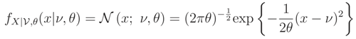
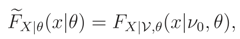
We consider the problem of inference on a parameter of interest θ of a probability distribution when we have some prior information on a nuisance parameter ν from a finite number of samples of this probability distribution. Assume that we know the expressions of either the cumulative distribution function (cdf) F_X|ν,θ(x|ν, θ) or its corresponding probability density function (pdf) f_X|ν,θ(x|ν, θ), X = (X₁, … ,X_n)′ and x = (x₁, … ,x_n)′. $𝒱$ is a random parameter on which we have an a priori information and θ is a fixed unknown parameter. This prior information can either be of the form of a prior cdf F_$𝒱$(ν) (or a pdf f_$𝒱$(ν)) or, for example, only the knowledge of a finite number of its moments. In the first case, the marginal cdf

(1)

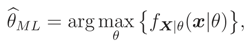
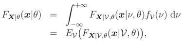is the classical tool for doing any inference on θ. For example the Maximum Likelihood (ML) estimate, ${\hat{\theta }}_{ML}$ of θ is defined as

where f_X|θ(x|θ) is the pdf corresponding to the cdf F_X|θ(x|θ).

In the second case the Maximum Entropy (ME) principle ([4, 5]), can be used for assigning the probability law f_$𝒱$(ν) and thus go back to the previous case, e.g. [1] page 90.

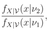
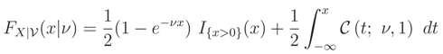
In this paper we consider the case where we only know the median of the nuisance parameter $𝒱$. If we had a complementary knowledge about the finite support of pdf of $𝒱$, then we could again use the ME principle to assign a prior and go back to the previous case, e.g. [3]. But if we are given the median of $𝒱$ and if the support is not finite, then in our knowledge, there is not any solution for this case. The main object of this paper is to propose a solution for it. For this aim, in place of F_X|θ(x|θ) in (1), we propose a new inference tool ${\tilde{F}}_{\mathit{X}|\theta }$(x|θ) which can be used to infer on θ (we will show that ${\tilde{F}}_{\mathit{X}|\theta }$(x|θ) is a cdf under a few conditions). For example we can define

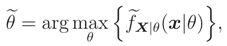where ${\tilde{f}}_{\mathit{X}|\theta }$(x|θ) is the pdf corresponding to the cdf ${\tilde{F}}_{\mathit{X}|\theta }$(x|θ).

This new tool is deduced from the interpretation of F_X|θ(x|θ) as the mean value of the random variable T = T ($𝒱$; x) = F_X|θ(x|θ) as given by (1). Now, if in place of the mean value, we take the median, we obtain this new inference tool ${\tilde{F}}_{\mathit{X}|\theta }$(x|θ) which is defined as

and can be used in the same way to infer on θ.

As far as the authors know, there is no work on this subject except recently presented conference papers by the authors, [9, 8, 7]. In the first article we introduced an alternative inference tool to total probability formula, which is called a new inference tool in this paper. We calculated directly this new inference tool (such as Example A in Section 2) and a numerical method suggested for its approximation. In the second one, we used this new tool for parameter estimation. Finally, in the last one, we reviewed the content of two previous papers and mentioned its use for the estimation of a parameter with incomplete knowledge on a nuisance parameter in the one dimensional case. In this paper we give more details and more results with proofs using weaker conditions, with a new overlook on the problem. We also extend the idea to the multivariate case. In the following, first we give more precise definition of ${\tilde{F}}_{\mathit{X}|\theta }$(x|θ). Then we present some of its properties. For example, we show that under some conditions, ${\tilde{F}}_{\mathit{X}|\theta }$(x|θ) has all the properties of a cdf, its calculation is very easy and depends only on the median of prior distribution. Then, we give a few examples and finally, we compare the relative performances of these two tools for the inference on θ. Extensions and conclusion are given in the last two sections.

2 A New Inference Tool

Hereafter in this section to simplify the notations we omit the parameter θ, and we assume that the random variables X_i, i = 1, … , n and random parameter $𝒱$ are continuous and real. We also use increasing and decreasing instead of non-decreasing and non-increasing respectively.

Definition 1

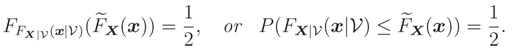
Let X = (X₁, … , X_n)′ have a cdf F_X|ν(x|ν) depending on a random parameter $𝒱$ with pdf f_$𝒱$(ν), and let the random variable T = T($𝒱$; x) = F_X|ν(x|$𝒱$) have a unique median for each fixed x. The new inference tool, ${\tilde{F}}_{\mathit{X}}(\mathit{x})$, is defined as the median of T:

(2)

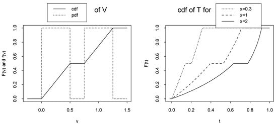
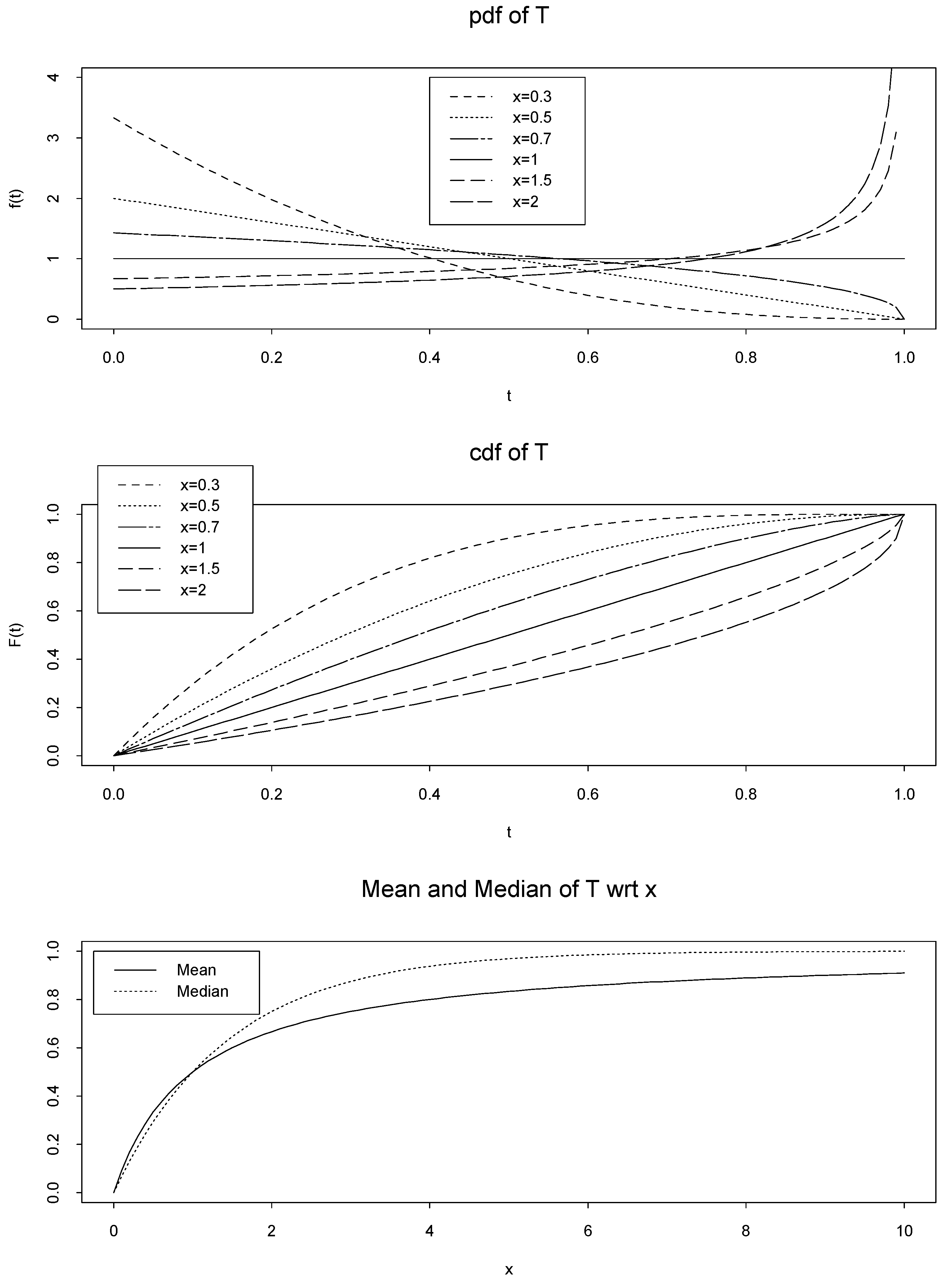
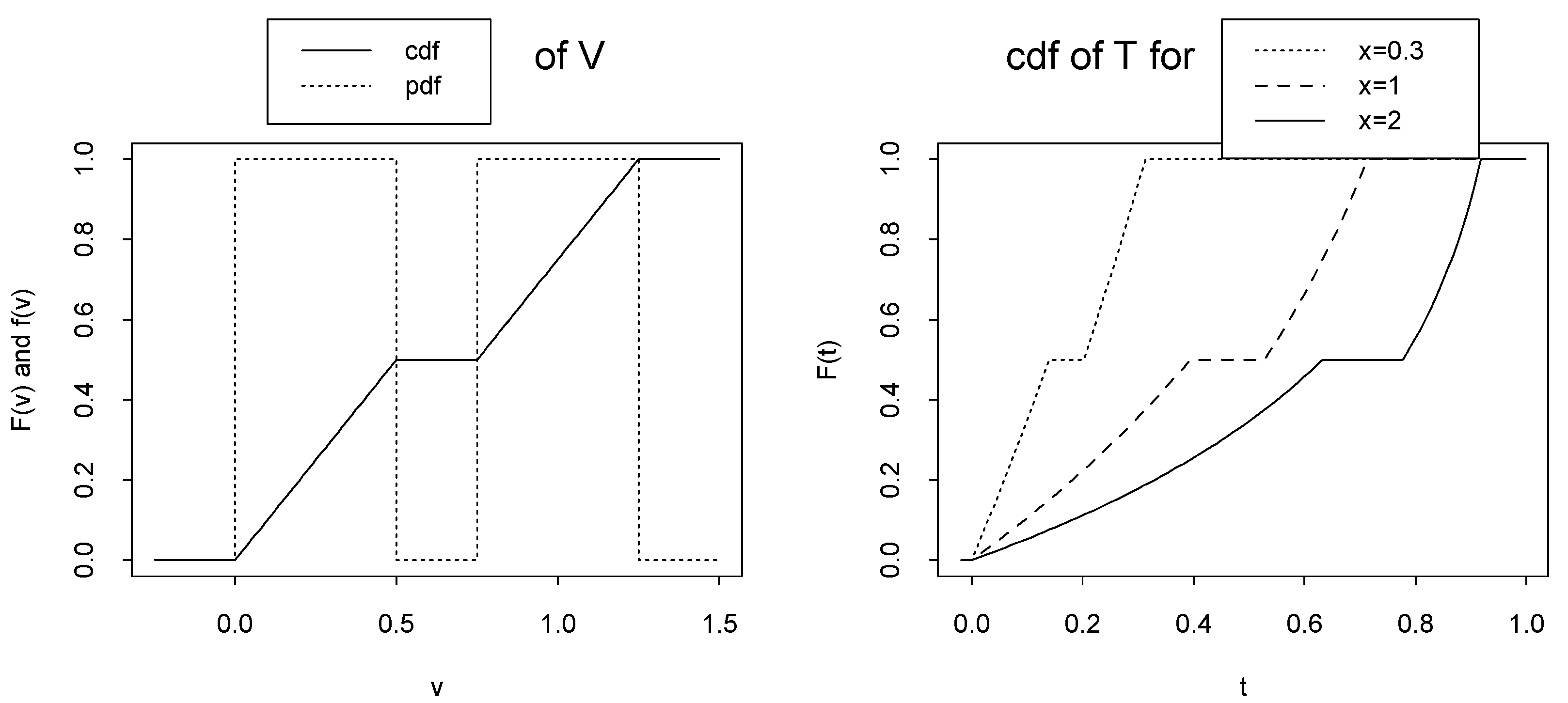
To make our point clear we begin with the following simple example, called Example A. Let F_X|$𝒱$(x|ν) = 1 − e^−νx, x > 0, be the cdf of an exponential random variable with scale parameter ν > 0. We assume that the prior pdf of $𝒱$ is known and also is exponential with parameter 1, i.e. f_ν(ν) = e^−ν, ν > 0. We define the random variable T = F_X|$𝒱$(x|$𝒱$) = 1 − e^−$𝒱$x, for any fixed value x > 0. The random variable 0 ≤ T ≤ 1 has the following cdf

Therefore, pdf of T is f_T(t) = $\frac{1}{x}$(1 − t)^{($\frac{1}{x}$ − 1)}, 0 ≤ t ≤ 1. Now, we can calculate the mean of the random variable T as follow

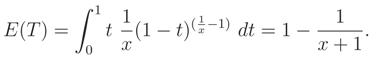
Let Med(T) be the median of the random variable T, then it can be calculated by

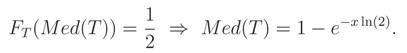
Mean value of the random variable T is a cdf with respect to (wrt) x. This fact is always true; because E(T) is the marginal cdf of random variable X, i.e. F_X(x). The marginal cdf is well known, well defined and can also be calculated directly by (1). On the other hand, in this example, it is obvious that Med(T) is a cdf wrt x, which is called ${\tilde{F}}_X$(x) in Definition 1, see Figure 1. However, we have not a short cut for calculating ${\tilde{F}}_X$(x) such as F_X(x) in (1).

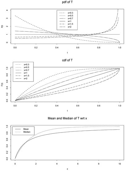
Figure 1. Top: pdf of random variable T = T ($𝒱$; x) = F_X|$𝒱$(x|$𝒱$) = 1 − e^−$𝒱$x, Middle: cdf of random variable T, and Bottom: mean and median of random variable T in Example A.

In the following theorem and remark, first we show that under a few conditions, ${\tilde{F}}_{\mathit{X}}$(x) has all the properties of a cdf. Then, in Theorem 2, we drive a simple expression for calculating ${\tilde{F}}_{\mathit{X}}$(x) and show that, in many cases, the expression of ${\tilde{F}}_{\mathit{X}}$(x) depends only on the median of the prior and can be calculated simply, see Remark 2. In Theorem 3 we state separability property of ${\tilde{F}}_{\mathit{X}}$(x) versus exchangeability of F_X(x).

Theorem 1

Let X have a cdf F_X|ν(x|ν) depending on a random parameter $𝒱$ with pdf f_$𝒱$(ν) and the real random variable T = F_X|ν(x|$𝒱$) have a unique median for each fixed x. Then:

1.

${\tilde{F}}_{\mathit{X}}$(x) is an increasing function in each of its arguments.

2.

If F_X|ν(x|ν) and F_$𝒱$(ν) are continuous cdfs then ${\tilde{F}}_{\mathit{X}}$(x) is a continuous function in each of its arguments.

3.

0 ≤ ${\tilde{F}}_{\mathit{X}}$(x) ≤ 1.

Proof: 

1.

Let y = (y₁, … , y_n)′, z = (z₁, … , z_n)′, y_j < z_j for fixed j and y_i = z_i for i ≠ j, 1 ≤ i, j ≤ n and take

Then using (2) we have

We also have Y ≤ Z, because F_X|$𝒱$ is an increasing function in each of its arguments. Therefore,

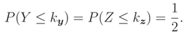k_y is the unique median of Y and so k_y ≤ k_z or equivalently ${\tilde{F}}_{\mathit{X}}$(x) is increasing in its j-th argument.

2.

Let x. = (x₁, … , x_{j − 1}, x., x_{j + 1}, … ,x_n)′ and t = (x₁, … , x_{j − 1}, t, x_{j + 1}, … ,x_n)′. By part 1, ${\tilde{F}}_{\mathit{X}}$(x) is an increasing function in each of its arguments. Therefore,

exist and are finite, e.g. [11].

Further, F_X|$𝒱$(x|$𝒱$) is continuous wrt x_j, and so

and by (2) we have

(3)

But ${\tilde{F}}_{\mathit{X}}$(x) is the unique median of F_X|$𝒱$(x|$𝒱$), therefore by (3),

and thus ${\tilde{F}}_{\mathit{X}}$(x) is continuous.

3.

${\tilde{F}}_{\mathit{X}}$(x) is the median of random variable T, where T = F_X|$𝒱$(x|$𝒱$) and 0 ≤ T ≤ 1, and so 0 ≤ ${\tilde{F}}_{\mathit{X}}$(x) ≤ 1.   ☐

Remark 1

By part 1 of Theorem 1, lim_xj↑+∞ ${\tilde{F}}_{\mathit{X}}$(x) and lim_xj↓−∞ ${\tilde{F}}_{\mathit{X}}$(x) exist and are finite, [11]. Therefore ${\tilde{F}}_{\mathit{X}}$(x) is a continuous cdf if conditions of Theorem 1 hold and

1.

lim_xj↓−∞ ${\tilde{F}}_{\mathit{X}}$(x) = 0 for any particular j,

2.

lim_{x1↑+∞,… ,xn↑+∞} ${\tilde{F}}_{\mathit{X}}$(x) = 1,

3.

∆_b1a1 …∆_bnan ${\tilde{F}}_{\mathit{X}}$(x) ≥ 0, where a_i ≤ b_i, i = 1, … , n, and ∆b_ja_j ${\tilde{F}}_{\mathit{X}}$(x) = ${\tilde{F}}_{\mathit{X}}$((x₁, … , x_{j − 1}, b_j, x_{j + 1}, … ,x_n)′)−${\tilde{F}}_{\mathit{X}}$((x₁, … , x_{j − 1}, a_j, x_{j + 1}, … ,x_n)′) ≥ 0.

In this case, we call ${\tilde{F}}_{\mathit{X}}$(x) the marginal cdf of X based on median. When ${\tilde{F}}_X$(x) is a one dimensional cdf, the last condition follows from parts 1 and 3 of Theorem 1.

Theorem 2

If L(ν) = F_X|ν(x|ν) is a monotone function wrt ν and $𝒱$ has a unique median $F_{\mathrm{𝒱;}}^{-1}\left(\frac{1}{2}\right)$, then ${\tilde{F}}_{\mathit{X}}$(x) = L($F_{\mathrm{𝒱;}}^{-1}\left(\frac{1}{2}\right)$).

Proof: 

Let

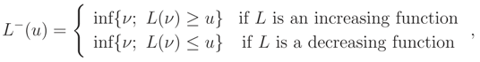be the generalized inverse of L, e.g. [10] page 39. Noting that

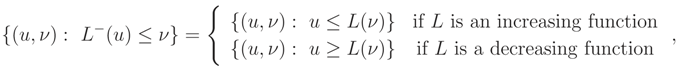and by (2) we have,

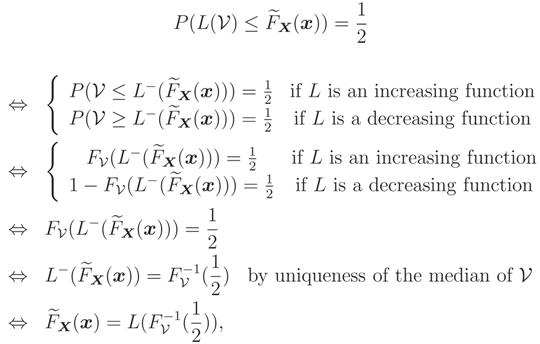where the last expression follows from

☐

Remark 2

If conditions of Theorem 2 hold, then ${\tilde{F}}_{\mathit{X}}$(x) belongs to the family of distributions F_X|$𝒱$(x|$𝒱$). Because, ${\tilde{F}}_{\mathit{X}}$(x) = F_X|ν(x|$F_{\mathrm{𝒱;}}^{-1}(\frac{1}{2})$) Therefore ${\tilde{F}}_{\mathit{X}}$(x) is a cdf and conditions in Remark 1 hold.

Remark 3

${\tilde{F}}_{\mathit{X}}$(x) depends only on the median of prior distribution, $F_{\mathrm{𝒱;}}^{-1}\left(\frac{1}{2}\right)$, while the expression of F_X(x) needs the perfect knowledge of F_$𝒱$(ν). Therefore, ${\tilde{F}}_{\mathit{X}}$(x) is robust relative to prior distributions with the same median.

Remark 4

If median of T is not unique then ${\tilde{F}}_X$(x) may not be a unique cdf wrt x. For example (called Example B), assumethat $𝒱$ has the following cdf, in Example A, Figure 2-left:

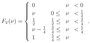Then, T = T ($𝒱$; x) = F_X|$𝒱$(x|$𝒱$) = 1 − e^−$𝒱$x has the following cdf

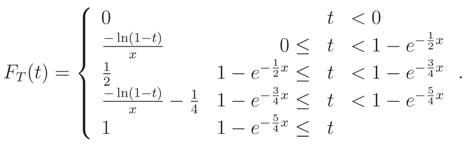Therefore, the median of T is an arbitrary point in the following interval: (see Figure 2-right)

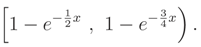
Figure 2. Left: cdf of random variable $𝒱$ in Example B and its corresponding pdf. Right: cdf of random variable T = T ($𝒱$; x) = F_X|$𝒱$(x|$𝒱$) = 1 − e^−$𝒱$x in Example B.

Theorem 3

Let F_X|ν(x|ν) be conditional cdf of X = (X₁, … , X_n)′ given $𝒱$ = ν and L_{(k1,… ,kr)}(ν) = F_{(Xk1 ,… ,Xkr)}|$𝒱$(x_k1 , … , x_kr|ν) be monotone function of ν for each {k₁, … , k_r} ⊆ {1, … , n}. Let also $𝒱$ have a unique median $F_{\mathrm{𝒱;}}^{-1}\left(\frac{1}{2}\right)$. If for each {k₁, … , k_r} ⊆ {1, … , n},

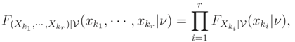i.e. X | $𝒱$ = ν has independent components, then

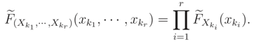
Proof: 

Conditions of Theorem 2 hold and so, for each {k₁, … , k_r} ⊆ {1, … , n},

☐

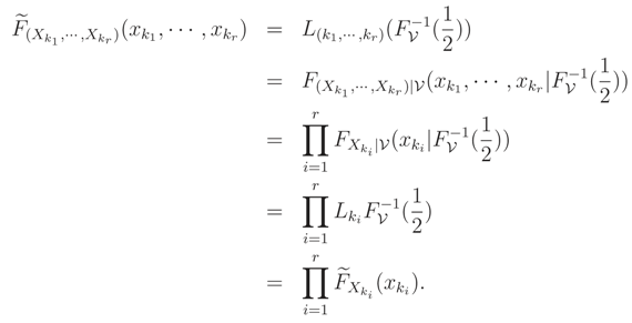Remark 5

If X | $𝒱$= ν has independent components, then the marginal distribution of X cannot have independent components. For example, in general case,

It can be shown that, if X | $𝒱$= ν has Independent and Identically Distributed (iid) components, then the marginal distribution of X is exchangeable, see Example 1. We recall that for identically distributed random variables exchangeability is a weaker condition than independence.

In the following we show that some families of distributions (e.g. [6]) have a monotone distribution function wrt their parameters and so, calculation of ${\tilde{F}}_{\mathit{X}}$(x) is very easy by using Theorem 2.

Lemma 1

Let L(ν) = F_X|$𝒱$(x|$𝒱$). If ν is a real location parameter then L(ν) is decreasing wrt ν.

Proof: 

Let ν₁ < ν₂ and ν be a location parameter. Then

☐

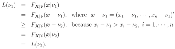Lemma 2

Let L(ν) = F_X|$𝒱$(x|ν). If ν is a scale parameter then L(ν) is monotone wrt ν.

Proof: 

Let ν₁ < ν₂. If ν is a scale parameter, ν > 0, then

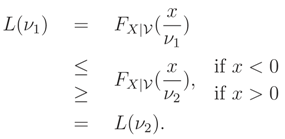Therefore, L(ν) is an increasing function if x < 0 and is a decreasing function if x > 0, i.e. L(ν) is a monotone function wrt ν. ☐

The proof of the following lemma is straightforward.

Lemma 3

Let X₁, … X_n given $𝒱$ = ν beiid random variables and X = (X₁, … , X_n)′. If L(ν) = F_X1|$𝒱$(x|ν) is an increasing (a decreasing) function then L*(ν) = F_X|ν(x|ν) is an increasing (a decreasing) function of ν.

In some cases we can show directly that L(.) is a monotone function. For example, in the exponen-tial family this property can be proved by using differentiation. Let X|η be distributed according to an exponential family with pdf

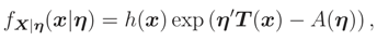where η = (η₁, … , η_n)′ and T = (T₁, … , T_n)′. It can be shown that L(η) = F_X|η(x|η) is a monotone function wrt each of its arguments in many cases by the following method: Let I_y≤x = 1 if y₁ ≤ x₁, … , y_n ≤ x_n and 0 elsewhere; and note that the differentiation under the integral sign is true for exponential family. Then

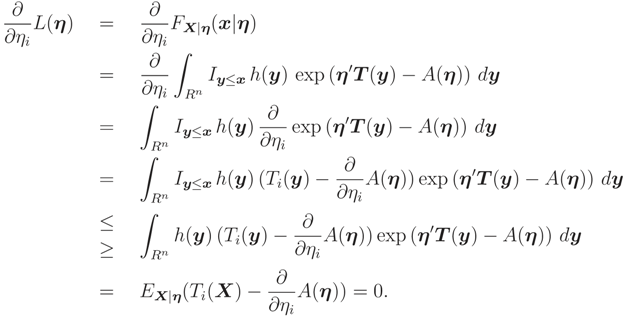The last equality follows from 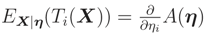, e.g. [6] page 27.

On the other hand, we can use stochastic ordering property of a family of distributions for showing that L(.) is a monotone function. A family of cdfs

(4)

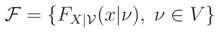where V is an interval on the real line, is said to have Monotone Likelihood Ratio (MLR) property if, for every ν₁ < ν₂ in V the likelihood ratio

is a monotone function of x. The property of MLR defines a very strong ordering of a family of distributions.

Lemma 4

If $ℱ$ is an MLR family wrt x then F_X|$𝒱$(x|ν) is an increasing (or a decreasing) functionof ν for all x.

Proof: 

See e.g. [12] page 124. ☐

A family of cdfs in (4) is said to be stochastically increasing (SI) if ν₁ < ν₂ implies F_X|$𝒱$(x|ν₁) ≥ F_X|$𝒱$(x|ν₂) for all x. For stochastically decreasing (SD) the inequality is reversed. This definition is a weaker property than MLR property (by Lemma 4), but is a stronger property than monotonicity of L(ν) = F_X|$𝒱$(x|ν) (because L(ν) is monotone for each fixed x). Therefore, we have

MLR ⇒ SI or SD ⇒ L(ν) is monotone

It can be shown that the converse of the above relations are not true.

Remark 6

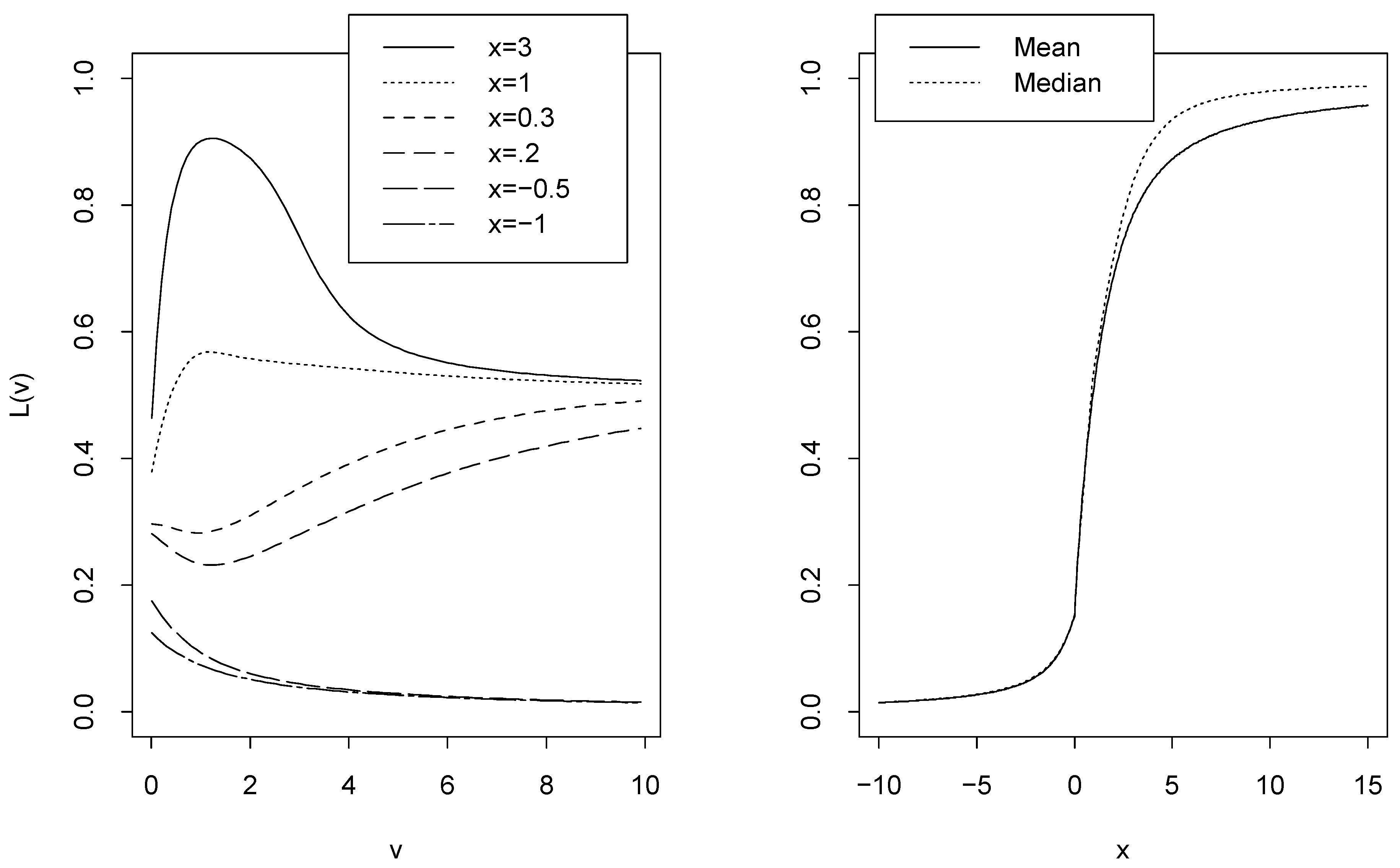
In Theorem 1, we prove that ${\tilde{F}}_X$(x) is an increasing function. In the proof of this theorem we do not use the monotonicity property of L(ν) = F_X|$𝒱$(x|ν) wrt ν.Forexample (called Example C), assume that

be mixture cdf of an exponential and a Cauchy cdf with parameter ν > 0. Figure 3-left shows the graphs of L(ν) = F_X|$𝒱$(x|ν) for different x. L(ν) is not monotone for some of x values in this figure. If we assume that the prior pdf of $𝒱$ is known and is also exponential with parameter 1, then, still median of random variable T is a cdf, see Figure 3-right.

Figure 3. Left: the graphs of L(ν) = F_X|$𝒱$(x|$𝒱$) for different x in Example C. Right: the mean and median of random variable T in Example C.

3 Examples

In what follows, we use the following notations and expressions, [2] pages 427-422:

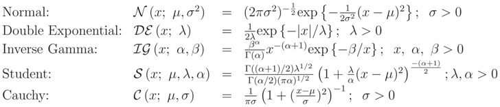Exchangeable Normal: The random vector X = (X₁, … , X_n)′ is said to have an exchangeable normal distribution, $ℰ$$𝒩$ (x; µ, σ², ρ), if its distribution is multivariate normal with the following mean vector and variance-covariance matrix

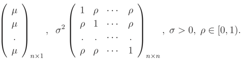It can be shown that $ℰ$$𝒩$ (x; µ, σ², ρ) =

where

3.1 Example 1

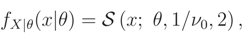
The first example we consider is

where we assume that the mean value ν is the nuisance parameter. Let X₁, … , X_n be an iid copy of X (i.e. X|$𝒱$ = ν, θ) and X = (X₁, … , X_n)′, then:

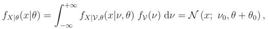
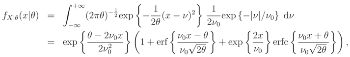
• Prior pdf case f_$𝒱$(ν) = $𝒩$ (ν; ν₀, θ₀):
  Then we have

  

  and

  
• Unique median knowledge case Median {$𝒱$} = ν₀:
  Then, as we could see, by using Lemma 1 and Theorem 2, we have

  

  or equivalently,

  

  Now we can use Theorem 3 for calculating ${\tilde{F}}_{\mathit{X}|\theta }$(x|θ) (because F_X|$𝒱$,θ(x|ν, θ) is a decreasing function wrt ν by Lemma 1), therefore,

  

  (5)

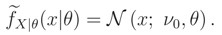  Note that, if f_$𝒱$(ν) = $𝒩$ (ν; ν₀, θ₀) or f_$𝒱$(ν) = $𝒞$ (ν; ν₀, θ₀) then ${\tilde{f}}_{\mathit{X}|\theta }$(x|θ) is given by (5), because the median of these two distributions are equal to ν₀ (see Remark 3).
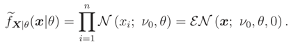
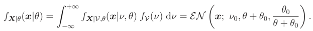
• Moments knowledge case E(|$𝒱$|) = ν₀:
  Then the ME pdf is given by $𝒟$$ℰ$ (ν; ν₀). In this case we cannot obtain an analytical expression for

  

  where We recall that, if we know that E($𝒱$) = ν₀ or Median {$𝒱$} = ν₀ and the support of $𝒱$ is R the ME pdf does not exist.

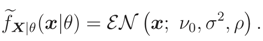
3.2 Example 2

The second example we consider is

where, this time, we assume that ν is the variance and the nuisance parameter. Then:

• Prior pdf case f_$𝒱$(ν) = $ℐ$$𝒢$ (ν; α, β):
  Then, it is easy to show that,

  

  (6)

  but f_X|θ(x|θ) cannot be calculated analytically.
• Unique median knowledge case Median {$𝒱$} = ν₀:
  Then, as we could see, by using Lemma 2 and Theorem 2, we have

  

  It can be shown that F_X|ν,θ(x|ν, θ) is a monotone function wrt ν (by using derivative) and by Theorem 3 we have

  
• Moments knowledge case E(1/$𝒱$) = 1/ν₀:
  Then, knowing that the variance is a positive quantity, the ME pdf f_$𝒱$(ν) is an $ℐ$$𝒢$ (ν; 1, ν₀). In this case we have

  

  and f_X|θ(x|θ) cannot be calculated analytically.

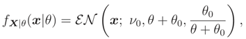
3.3 Example 3

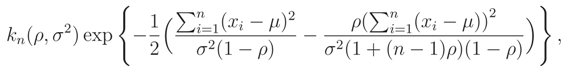
In this example we consider is $ℰ$$𝒩$ (x; ν, σ², ρ), where ν is a nuisance parameter. Noting that, we can write $ℰ$$𝒩$ (x; ν, σ², ρ), as follows (exponential family),

where , can be determined. This pdf is a monotone function wrt θ₃ and so L(ν) is a monotone function. Let θ = (σ², ρ) and the median of prior pdf be ν₀, then

3.4 Comparison of Estimators in Example 1

Suppose we are interested in estimating θ in Example 1. In the case that n = 1

and so the ML estimator (MLE) of θ based on these two pdfs are equal to

respectively. For n > 1 the MLE of θ based on

can be calculated numerically by the following simplified likelihood function,

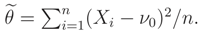
where we assume that θ₀ = 1. The MLE of θ based on , is equal to

Before comparing these two estimators (by considering normal prior for ν), one can predict that, $\hat{\theta }$ is better than $\tilde{\theta }$, because $\hat{\theta }$ uses more information (i.e. known normal prior) than $\tilde{\theta }$ which uses only the median of prior distribution. We may also recall that, f_X|θ(x|θ) is the true pdf of observations obtained using the full prior knowledge on the nuisance parameter, while ${\tilde{f}}_{\mathit{X}|\theta }$(x|θ) is a pseudo pdf which includes only prior knowledge of the median of nuisance parameter.

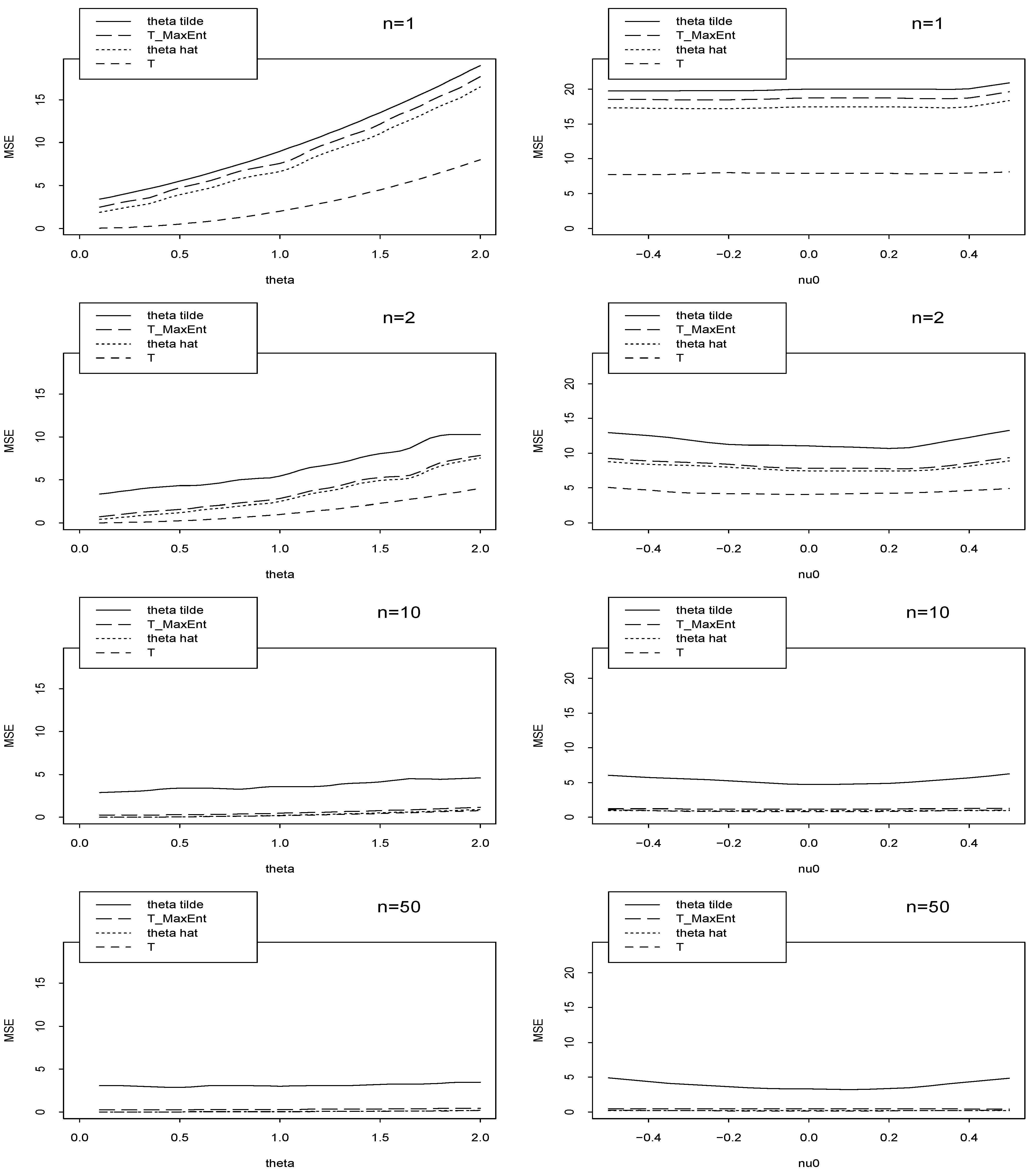
The empirical Mean Square Error (MSE) of 4 estimators are plotted in Figure 4 for different sample sizes n. We note by T the MLE of θ when ν = ν₀, and we note by T_MaxEnt the MLE of θ when the prior mean and variance are known.

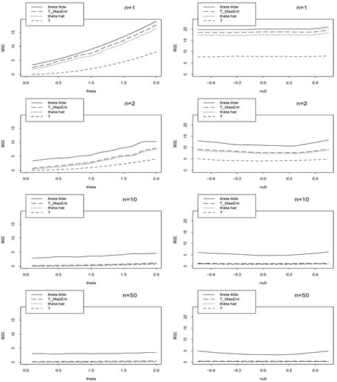
Figure 4. The empirical MSEs of $\tilde{\theta }$, T_MaxEnt, $\hat{\theta }$, and T wrt θ (left) and ν₀ (right, for θ = 2) for different sample sizes n.

In Figure 4-left we plot the graphs of MSE of $\hat{\theta }$, $\tilde{\theta }$, T and T_MaxEnt. In Table 1 we classify these 4 estimators and corresponding assumptions for n = 1. We see that, in Figure 4-left, $\hat{\theta }$ is better than $\tilde{\theta }$, especially for large sample size n, and T is the best.

Table 1. Comparing estimators of variance in four different situations.

Assumptions	pdf of X|θ based on prior information MLE of θ	Simulated data pdf MSE(θ) = E(MLE − θ)2
Known parameter ν = ν0	$𝒩$ (x; ν0, θ) T = (X − ν0)2	$𝒩$ (x; 0, θ) 2θ2
Known prior f$𝒱$(ν) = $𝒩$ (ν; ν0, θ0)	$𝒩$ (x; ν0, θ + θ0) $\hat{\theta }$ = max{(X − ν0)2 − θ0, 0}	$𝒩$ (x; 0, θ + 1) E($\hat{\theta }$ − θ)2
Known moments E($𝒱$) = ν0, V ($𝒱$) = $\frac{{\theta }_0}{2}$	$𝒩$ (x; ν0, θ + $\frac{{\theta }_0}{2}$) TMaxEnt = max{(X − ν0)2 − $\frac{{\theta }_0}{2}$, 0}	$𝒩$ (x; 0, θ + 1) E(TMaxEnt − θ)2
Known unique median Median($𝒱$) = ν0	$𝒩$ (x; ν0, θ) $\tilde{\theta }$ = (X − ν0)2	$𝒩$ (x; 0, θ + 1) 2(θ + 1)2 + 1

In Figure 4-right we plot the graphs of MSE wrt median, ν₀. This is useful for checking robustness of estimators wrt false prior information. We see that $\hat{\theta }$ is more robust than $\tilde{\theta }$ relative to ν₀, but both of them dominated by T. In this case, samples are generated from a normal distribution with random normal mean (median ν₀) when θ = 2, however, we assume that ν has a standard normal prior distribution.

The simulations confirm the following logic: more we have information better will be the estima-tion. In fact for calculating T we have not nuisance parameter; for $\hat{\theta }$, we use all prior distribution information; for T_MaxEnt we use prior mean and prior variance information; and for $\tilde{\theta }$ we use only the median value of prior distribution.

4 Extensions

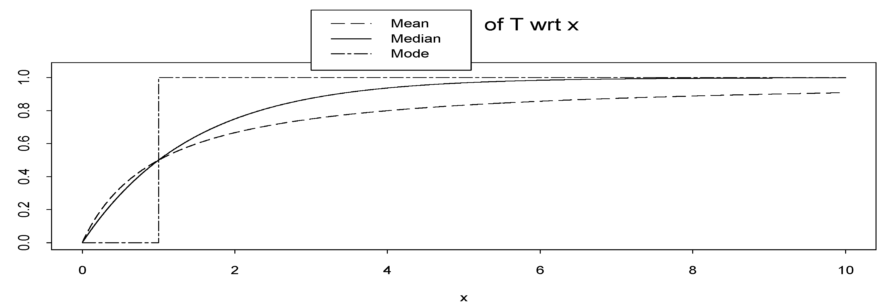
In this section, we show that the suggested new tool can be extended to other functions such as quantiles instead of median, but not to other functions such as mode. For example, mode of the random variable T = T ($𝒱$; x) = F_X|$𝒱$(x|θ) in Definition 1, i.e.,

(7)

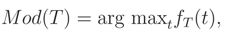is not a cdf in Example A. The mode of T is: (see Figure 1 top)

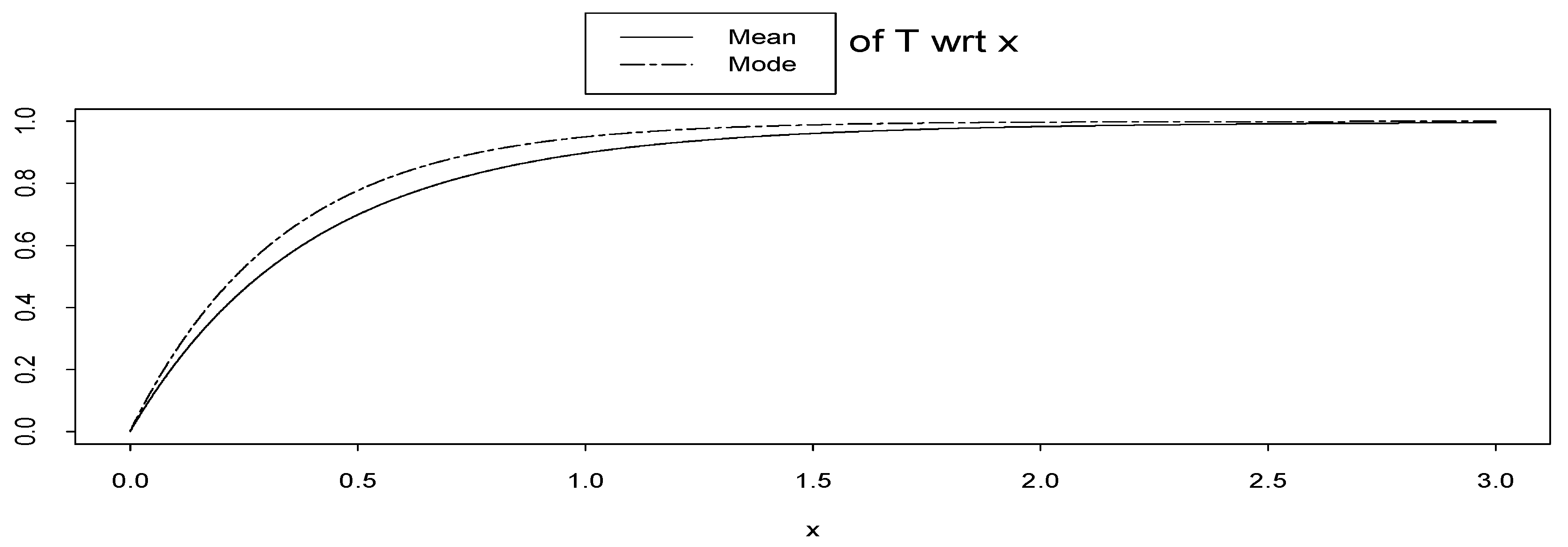
which is not a distribution function. If we assume k = 1, then Mod(T) is a degenerate cdf. In Figure 5 we plot the mean, median and mode of the random variable T. We see that they are cdfs. However, the cdf based on mode is the extreme case of the two others.

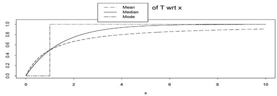
Figure 5. Mean, median and mode of random variable T = T ($𝒱$; x) = F_X|$𝒱$(x|$𝒱$) = 1 − e^−$𝒱$x wrt x.

As noted by one of the referees, the mode of prior pdf is useful for introducing a pseudo cdf similar to our new inference tool, ${\tilde{F}}_{\mathit{X}}$(x). That is, instead of using the result of Theorem 2: ${\tilde{F}}_{\mathit{X}|\theta }$(x|θ) = F_X|ν,θ(x|Med($𝒱$), θ), using ${\tilde{F}}_{\mathit{X}|\theta }^{\mathit{Mod}}$(x|θ) = F_X|ν,θ(x|Mod($𝒱$), θ). This method was used for eliminating the nuisance parameter ν. In this case, Theorem 3, i.e. separability property of pseudo marginal distribution, also holds for ${\tilde{F}}_{\mathit{X}|\theta }^{\mathit{Mod}}$(x|θ). Note that, the mode of the random variable T, defined in (7) is not equal to ${\tilde{F}}_{\mathit{X}|\theta }^{\mathit{Mod}}$(x|θ) and may not be a cdf similar to the above illustration. However, it may be a cdf similar to the following example pointed out by the referee. In Example A, let $𝒱$ − 1 be a binomial distribution with parameters $ℬ$(2, $\frac{3}{4}$), i.e. $𝒱$ is a discrete random variable with support {1, 2, 3}. Then E(T) = 1 − (e^−x + 6e^−2x + 9e^−3x)/16 and Mod(T) = 1 − e^−3x are cdfs see Figure 6.

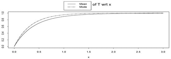
Figure 6. Mean and mode of random variable T = T ($𝒱$; x) = F_X|$𝒱$(x|$𝒱$) = 1 − e^−$𝒱$x wrt x.

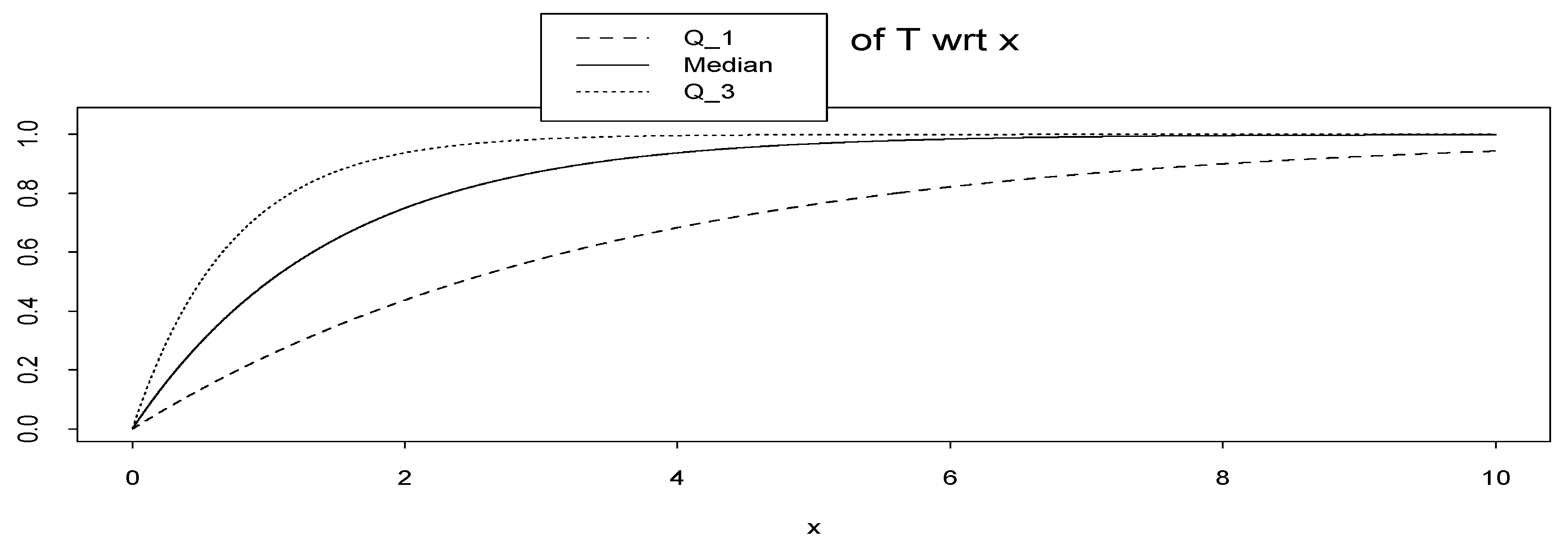
On the other hand, we may extend the method presented in this paper to the class of quantiles (e.g., quartiles or percentiles). To make our point clear we consider the first and third quartiles of random variable T in Example A (instead of median, which is the second quartile). We denote the new inference tools based on first and third quartiles by ${\tilde{F}}_{\mathit{X}|\theta }^{Q_1}$(x) and ${\tilde{F}}_{\mathit{X}|\theta }^{Q_3}$(x) respectively.

They can be calculated such as (2) by

It can be shown that, in Example A, ${\tilde{F}}_X^{Q_1}$(x) = 1 − e^{x ln 0.75} and ${\tilde{F}}_X^{Q_3}$(x) = 1 − e^{x ln 0.25}. In Figure 7 we plot them.

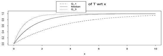
Figure 7. Q₁, median and Q₃ of random variable T = T ($𝒱$; x) = F_X|$𝒱$(x|$𝒱$) = 1 − e^−$𝒱$x wrt x.

In conclusion, it seems that the method can be extended to any quantiles instead of median, but its extension to other functions may need more care.

References

- Berger, J. O. Statistical Decision Theory: Foundations, Concepts, and Methods; Springer: New York, 1980. [Google Scholar]
- Bernardo, J. M.; Smith, A. F. M. Bayesian Theory; Wiley: Chichester, UK, 1994. [Google Scholar]
- Hernández Bastida, A.; Martel Escobar, M. C.; Vázquez Polo, F. J. On maximum entropy priors and a most likely likelihood in auditing. Qüestiió 1998, 22(2), 231–242. [Google Scholar]
- Jaynes, E. T. Information theory and statistical mechanics I,II. Physical review 1957, 106, 620–630. [Google Scholar] and 108, 171–190.
- Jaynes, E. T. Prior probabilities. IEEE Transactions on Systems Science and Cybernetics SSC-4 1968, (3), 227–241. [Google Scholar]
- Lehmann, E. L.; Casella, G. Theory of point estimation, 2nd ed.; Springer: New York, 1998. [Google Scholar]
- Mohammad-Djafari, A.; Mohammadpour, A. On the estimation of a parameter with incomplete knowledge on a nuisance parameter. 2004; Vol. 735, AIP; pp. 533–540. [Google Scholar]
- Mohammadpour, A.; Mohammad-Djafari, A. An alternative criterion to likelihood for parameter estimation accounting for prior information on nuisance parameter. In Soft methodology and Random Information Systems; Springer: Berlin, 2004; pp. 575–580. [Google Scholar]
- Mohammadpour, A.; Mohammad-Djafari, A. An alternative inference tool to total probability formula and its applications. 2004; Vol. 735, AIP; pp. 227–236. [Google Scholar]
- Robert, C. P.; Casella, G. Monte Carlo statistical methods, 2nd ed.; Springer: New York, 2004. [Google Scholar]
- Rohatgi, V. K. An Introduction to Probability Theory and Mathematical Statistics; Wiley: New York, 1976. [Google Scholar]
- Zacks, S. Parametric statistical inference; Pergamon, Oxford, 1981. [Google Scholar]
© 2006 by MDPI (http://www.mdpi.org). Reproduction for noncommercial purposes permitted.