Mechanics and Ensembles.
The conception of Gibbs's ensemble [
1] is known to be the basis of statistical mechanics, with equations of mechanics being used in the form of Liouville's equation. This differential equation in partial derivatives of the first order is equivalent to Hamilton's equations. Still the conception of Gibbs’s ensemble, which proved valid in the equilibrium case, does not lead to satisfactory results in an attempt to generalize it for the general case.
No one has succeeded in finding a non-trivial solution of Liouville's equation up to now. Moreover, a possibility to give a correct definition of entropy for a nonequilibrium case is doubtful. That Gibbs's definition of entropy fails to suit for general case, is clearly seen from considering the distribution function for a canonical ensemble, since temperature of the system in question [
1] enters the formula of Gibbs's entropy in terms of this distribution function. However, in the nonequilibrium case the system can have different temperatures in its diverse parts or it can even be characterized by a temperature field.
The application of Gibbs's ensemble to a part of the system is invalid by the following reason: in constructing the Gibbs's ensemble, the coordinates of external bodies are considered to be equal (and macroscopical) for all the ensemble forming systems. In this case, the system can only exchange work with its environment but not heat, so it is adiabatic. The content of this statement will be lighted up further in the course of interpretation. The Gibbs's ensemble, therefore, is not the most general one, and a view about the canonical Gibbs's distribution as describing the system in the thermostat is not exactly correct. The nature of this discrepancy will be elucidated later. Taking into account the above, it is reasonable from the very beginning to construct the classical statistical mechanics on the conception of ensemble which is more general than the Gibbs's ensemble. Such an ensemble should consist of systems, more exactly of subsystems, exchanging with the environment not only work but also heat.
For this purpose, it is necessary and sufficient to assume that coordinates and momenta of external bodies, i.e. particles surrounding the subsystem under consideration, might have different values for each of the subsystems. Any nonequilibrium thermodynamic system can be presented as consisting of such subsystems being infinitely small in general case. It is implied that all the systems are under similar macroscopical conditions which can be characterized by assigning fields of thermodynamic parameters. If we manage to define the entropy for any subsystem so that it could change owing to exchange of heat with the surrounding subsystems, then the entropy of the whole system can change in integral considering the whole system, similarly to the case with thermodynamic consideration. Hereinafter such an ensemble is referred to as the ensemble of subsystems. Thus, let us consider the ensemble of subsystems and define the equations for its evolution to be described.
To construct the ensemble of subsystems, let us consider any thermodynamic system, whose state is assumed to be given "macroscopically", and take conceptually an infinite number of its copies characterized by the same thermodynamic parameters. Let each system consist of N particles. Mentally single out a subsystem of n particles (1 ≤ n < N) from every system and represent it as a point in the phase space of dimension 6n. In this case we consider coordinates and momenta of external (for the subsystem) particles as assigned, though unknown. Generally speaking, they will be different for each subsystem. With this, the phase volume occupied by the singled out set of phase points in the space of dimension 6n, will change with time. At first glance, this statement is contrary to the well known theorem of the phase volume conservation by Hamiltonian systems.
Actually there is no contradiction, and the use of the mentioned theorem does make the result to be almost obvious. To understand this, one should otherwise approach the construction of the ensemble of subsystems: it may be grasped that the above ensemble presents a projection of section of Gibbs's ensemble of dimension 6N by a hypersurface, on a subspace of dimension 6n. But it in no way follows that the projection area of the singled out part of the section will not change with time
We now proceed to analytical consideration of the problem. Consider the ensemble of subsystems, the evolution of each of them being defined by Hamilton's equations:
where
qα is 3n of generalized coordinates,
pα is 3n of generalized momenta
H = H(q1,…q3N,p1,…p3N,t) is the Hamiltonian of the whole system, which depends on 3N coordinates and momenta of all N particles and, probably, on time t.
Now we are to show that
that is the phase volume calculated at the time point
t0 is not equal to the corresponding phase volume calculated at the time point
t ≠
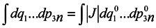
t0. To do this, it would seem possible to use a well-known technique of change from integration with respect to one set of variables to integration with respect to another one using the Jacobian
and to write with denoting the multiple integration by one symbol ∫
To use this formula, however, it is necessary that one-to-one correspondence would exist between the positions of the phase point at moments
t and
t0.
In this case, generally speaking, there is no such a correspondence (which requires a change to a statistical description by itself). Nevertheless, such a correspondence is certain to take place at start time and J0 = 1, i.e. formula (2) holds for the case of subsystems for infinitesimal transformations. Let us show that dJ/dt is not equal to zero identically. To make it obvious, first we consider the simplest case where the initial system involves only two particles executing one-dimensional motion. And we take one particle as the subsystem.
We are going to show that
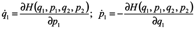
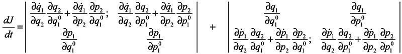
Differentiate
J with respect to time
Using Hamilton's equations:
one can write
and analogous expressions for
![Entropy 07 00122 i008]()
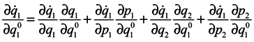
In expression (4) the presence of the third and fourth terms is very essential, which contain partial derivatives with respect to
q2 and
p2, i. e. with respect to coordinates and momenta of surrounding particles. When substituting (4) into (3), either of determinants is divided into the sum of four determinants, with determinants free of partial derivatives with respect to
q2 and
p2 being equal to zero (similarly to the case of Gibbs's ensemble [
1]), and combining the retaining terms we obtain:
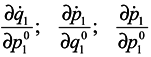
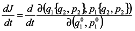
One can write the obtained results by convention in the form:
This notation means merely that differentiation of the kind
![Entropy 07 00122 i011]()
is made by way of intermediate variables
q2 and
p2 and the variables
q1 and
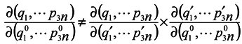
pp are lost. It is seen that in general case
![Entropy 07 00122 i012]()
Similarly. one can consider a more general case with systems of
N particles and subsystems of
n particles Calculations become more unwieldy, but the final result has the same form
where from here on indices
κ mark the numbers of coordinates and momenta of the system particles which don't belong to the subsystem under consideration. The meaning of the result consists in the fact that a contribution to changes of phase volume is made by those changes of
qα and
pα of coordinates and momenta of the subsystem particles, which are caused by interactions of the subsystem particles with environmental particles. It is obvious that in the limiting case of absence of subsystems interaction with the environment, we obtain the Gibbs's ensemble and the phase volume conservation. One can note that it is seen from equations (5) and (6) that a phase volume change for subsystems is not directly related to velocity divergence (see in more detail hereinafter). Moreover, from the above one can easily obtain that for the subsystems
where
are the coordinates at the time point
t′. This proves again that equation (2) is inapplicable in this case.
Introduce now the distribution function
ρn for the ensemble of subsystems of
n particles similarly to the case of Gibbs's statistics. This function defining probability of values of coordinates
qα and momenta
pα of
n subsystem particles can also depend on time
t and parametrically on coordinates
qκ and momenta
pκ of particles surrounding the subsystem. Therefore the total derivative of the distribution function
ρn with respect to time should be written in the form:
Consider now the possibility of applying a continuity equation in 6
n-space of the ensemble of subsystems. The absence of velocity spread in the phase space is the condition of application the continuity equation, i. e. at the infinitely near space points the velocity values are bound to differ by the infinitesimal [
2]. In this case the spreading may appear in the subspace of momenta
pα, for the velocity
in it represents a force acting on the particle. In principle, a situation is possible when at an infinitely small difference in the positions of two points in the 6
n-space, forces acting from the environment differ by a finite quantity due to a finite difference in the positions of surrounding particles. This case, however, can be easily avoided by means of proper choice of subsystems. For this purpose, there must be no discontinuity in the hypersurface intersecting Gibbs's ensemble so as to form an ensemble of subsystems, i. e. the hypersurface must be smooth. This condition is not essentially burdensome and we can use the continuity equation in the 6
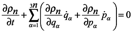
n-space as well, where it takes the form
Using Hamilton's equations and the equality of second mixed derivatives, one can reduce equation (8) to the following form:
From the form of equation (9), it is bound seemingly to follow
, for the second member is equal to zero. Still, since
ρn depends, generally speaking, on 6
N variables and time, 6
N equations will be equations of characteristics for it, from them 6
n equations being of the form
and 6(
N −
n) equations of the form
The index
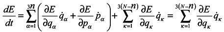
κ relates to coordinates and momenta of external particles, which are not constant but change according to Hamilton's equations. In view of this:
Substituting (9) into (7) we obtain
It is appropriate here to make a small digression and say about the relationship between velocity divergence and volume change. It is well-known Liouville's theorem from the theory of differential equations, according to which, with velocity divergence being equal to zero, the conservation of volumes takes place in mapping. This theorem is proved for the case when dimensionality of a volume whose change is considered in mapping, is equal to the number of variables and to the number of differential equations whose solutions perform mapping of the volume. But in this case we consider mapping of section of dimensionality 6
n, which are less than the total number 6
N of variables and differential equations.
In this case, the above theorem does not already take place. Instead of considering where exactly the conditions of theorem applicability are violated, we illustrate this by means of a simple example.
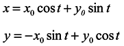
Let us consider a system of two equations and a one-dimensional ensemble in the X-direction
Here y is not a generalized momentum. A velocity divergence in the X-direction calculated from the first equation of the system (11) is equal to 0
And the general solution of the system (11) has the form
Hence, having assumed for simplicity
y0 = 0 we see that the length of any segment X-direction is not constant in time. That is in the one-dimensional ensemble under consideration, the volume is not conserved though the velocity divergence is equal to 0.
After this short digression, we turn again to equation (9), by its form it does not differ from Liouville's equation. There is an important distinction, however, consisting in the fact that terms of the form contain forces acting on particles of the subsystem in question from surrounding particles. Those are "dissipative" forces which on averaging, for example, can give forces proportional to velocity acting on Brownian particles, i.e. the considered approach allows one to build a bridge between Hamiltonian and dissipative systems. The same forces cause energy fluctuations in subsystems. Moreover, they are also responsible for other effects that will be considered below.
We now turn to the search of solutions of the equations. First for simplicity, we shall seek stationary solutions, i.e. those satisfying the condition
. Assume that Hamiltonian of the whole system does not explicitly depend on the time t and represent it in the form
where
H1(
qα,
pα) is energy of the subsystem under consideration without regard for the environment;
Hw(
qα,
qκ) is energy of interaction with the environment of the subsystem;
H2(
qκ,
pκ) is energy of the environment. For simplicity, we have supposed here
Hw as independent of momenta, which is not a principal restriction. Let us denote by
E the expression of the form
Then according to Hamilton's equations
Hence
The last equation is obtained in terms of (12).
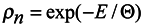
Now it is possible to write the simplest equation for the distribution function
ρn satisfying equations (9) and (10) as well as the condition
where Θ is the parameter, the meaning of which (temperature in energy units) will be revealed below.
Since according to the above assumption
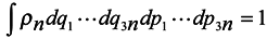
ρn is the distribution function of subsystems in the phase space, then it is subject to normalization to the unit.
where integration is performed over the whole phase space (6
n dim),
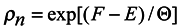
In accordance with the said above, we choose the distribution function in the form
where
F depends on Θ and
qκ , but not on
qα and
pα. So equations (9) and (10) are satisfied by the solution (15). This solution is a local, more exactly quasilocal distribution in the assigned field of temperatures, that depends on the environment. The environmental dependence enters through the interaction energy
Hw which provides fluctuations in an equilibrium case and evolution in a non-equilibrium case.
The limiting transfer to the canonical Gibbs's distribution is obvious. It is also clear that the canonical Gibbs's distribution is merely the limiting case of distribution in a thermostat at Hw → 0
Entropy
Consider expression (15) in more detail. This distribution function contains coordinates qκ as parameters, i.e. it is a conditional distribution function. But the values of qκ are unknown for us. Nevertheless, we can construct an ensemble for a neighboring subsystem and define probability of values of all the coordinates qκ or a part thereof. It is coordinates qα of the first subsystem that will now enter into the distribution function as parameters. We can not generally establish such boundary conditions for a subsystem that they should be independent of the subsystem itself. It is not a drawback of this method but presents a more general case of describing nature. Indeed, when we establish boundary conditions "strictly", we introduce certain idealization neglecting a reverse action of the system under consideration on the surroundings. It is clear that such idealization is not always permissible. Since (15) involves the interaction energy of subsystems, which reflects the fact that the subsystems are not statistically independent, then the distribution function of the whole system can not be obtained by factorization of distribution functions of the subsystems. However, with weak coupling being present, such an approximation is possible. Since in this case subsystem temperatures can differ, the total distribution function will not be symmetrical in respect to a rearrangement of coordinates of particles belonging to two different subsystems. Nevertheless, in rearranging particle coordinates within a subsystem, the distribution function will not change, i.e. a local symmetry takes place.
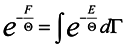
Now turn again to expression (14) and rewrite it taking into consideration (15)
where
dΓ =
dq1 …
dq3ndp1 …
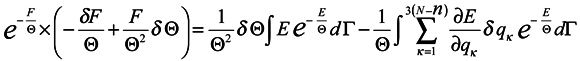
dp3n and take a variation from both sides of (16) in changing the coordinates
qκ and parameter Θ .
In doing this we assume vanishing the distribution function at boundaries of the integration domain:
The expression
![Entropy 07 00122 i034]()
represents the force acting on the environment particles by the subsystem. Now we multiply both sides of the obtained expression by exp(
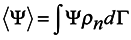
F/Θ) and use the formula for the average over the ensemble
where Ψ is an arbitrary function of the coordinate
qα and momenta
pα.
Then
Hence
Since it follows from (15) that
lnρn = [(
F −
E)/Θ]
then
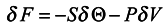
Comparing (17) with the expression for free energy /6/ known from local thermodynamics
we conclude that
S = −〈
lnρn〉 can be interpreted as local entropy in appropriate units, Θ is the subsystem temperature. The second term of expression (17) is related to the expansion work −
PδV where
P is pressure,
δV is the volume variation. A detailed analysis of the expression
![Entropy 07 00122 i040]()
will allow one to understand under what conditions the approximation of local thermodynamics for the expansion work is valid. Turning back to the definition of local entropy
![Entropy 07 00122 i041]()
we see that it is the same in form as the Gibbs's one but has somewhat another content. Now entropy is a dynamical variable changing in accordance with a change of
qκ and it is not a strictly additive value. In integral consideration of the whole nonequilibrium system, its entropy can increase. This problem requires further investigation. One circumstance, however, deserves mentioning. In the literature (e.g. [
6]) one can find a statement that in the local-equilibrium distribution the entropy can not increase. In our opinion, this statement is not true and is based on the fact that energy of interaction with the environment of the considered part of the system has not been properly taken into account. Moreover, from the above consideration it should be clear that for the mechanical substantiation of the second law of thermodynamics, there is no need in a non- physical assumption on discrepancy of calculated and measured trajectories, which was made in a widely cited paper by N. S. Krylov [
7].
Devoid of grounds is also the conclusion made by J. Prigogine in paper [
8] concerning the fact that in thermodynamic systems the basic concepts of classical and quantum mechanics cease to conform to experimental data.
Many manuals on statistical mechanics contain a derivation of hydrodynamical equations from Boltzmann's equation. Let us consider it in detail, following the work [
3]. Boltzmann's equation has the form
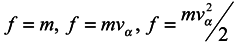
where
f =
f(
xα,
vα,
t) is one-particle distribution function,
xα are the particle coordinates,
vα are velocities,
Fα are components of a volume force affecting the particle.
Jc is the collision integral, the particular form of which is not very important for us. Now essential is just the fact that in this term, and only in it, all the interactions of the particle under consideration with the environment are taken into account.
The left-hand side of (18) represents a one-particle Liouville's equation for a molecule of the ideal gas. Equation (18) is transformed in a standard manner [
3] to Maxwell's transfer equation containing an arbitrary function
f of coordinates, time and velocities.
In the cases
![Entropy 07 00122 i043]()
the right-hand side of the transfer equation, which takes the
particle interaction into account, vanishes [
3]. In this connection we shall obtain the same equation that we would obtain if we initially began the derivation from the one-particle Liouville's equation in which account has been taken of only volume forces and by no means particle interaction forces have been taken into account, which being "dissipative" in averaging. Therefore, hydrodynamic equations obtained from Boltzmann's equation are those for ideal liquid. Accordingly, an expression for viscous stress tensor used in this derivation is formal and inexact. Also incorrect, in our opinion, is the conclusion based on this definition, that in an equilibrium state all the gases are non-viscous. One could equally well allege that masses of all the bodies at rest are equal to zero.


 is made by way of intermediate variables q2 and p2 and the variables q1 and pp are lost. It is seen that in general case


 represents the force acting on the environment particles by the subsystem. Now we multiply both sides of the obtained expression by exp(F/Θ) and use the formula for the average over the ensemble


 will allow one to understand under what conditions the approximation of local thermodynamics for the expansion work is valid. Turning back to the definition of local entropy
  we see that it is the same in form as the Gibbs's one but has somewhat another content. Now entropy is a dynamical variable changing in accordance with a change of qκ and it is not a strictly additive value. In integral consideration of the whole nonequilibrium system, its entropy can increase. This problem requires further investigation. One circumstance, however, deserves mentioning. In the literature (e.g. [6]) one can find a statement that in the local-equilibrium distribution the entropy can not increase. In our opinion, this statement is not true and is based on the fact that energy of interaction with the environment of the considered part of the system has not been properly taken into account. Moreover, from the above consideration it should be clear that for the mechanical substantiation of the second law of thermodynamics, there is no need in a non- physical assumption on discrepancy of calculated and measured trajectories, which was made in a widely cited paper by N. S. Krylov [7].
 the right-hand side of the transfer equation, which takes the