Entropy Analysis in Pipe Flow Subjected to External Heating

Abstract

In the present study, heat transfer and entropy analysis for flow through a pipe system is considered. The Reynolds number and the pipe wall temperature effects on entropy distribution and total entropy generation in the pipe are investigated. Numerical scheme employing a control volume approach is introduced when solving the governing equations. Steel is selected as pipe material, while water is used as fluid. It is found that increasing pipe wall temperature and Reynolds number increases the entropy production rate, in which case, entropy generation due to heat transfer dominates over that corresponding to fluid friction.

Introduction

Flow through pipes finds wide applications in industry. The flow and heat transfer characteristics can be further improved through studying irreversibilities associated in the flow system. The flow through pipes in thermal environment suffers from frictional and heat transfer losses; in which case, friction reduces the pressure; while heat transfer lowers the thermal efficiency of the piping system.

From the industrial application point of view, flow through piping system is turbulent which requires appropriate modeling to predict the flow properties. Considerably research studies were carried out to investigate the flow and heat transfer characteristics of pipe flow. Numerical simulation of transitional flow and heat transfer in smooth pipe was carried out by Huiren and Songling [1]. They indicated that in the fully developed region, flow and heat transfer were not affected by inlet turbulence intensities, and the agreement between the predictions and data for the friction coefficient was good. The behavior of friction and heat transfer coefficients of water flowing turbulently in a relatively long pipe was investigated by Choi and Cho [2]. They proposed a new turbulent heat transfer correlation for the local Nusselt number. Pressure drop and heat transfer in turbulent duct flow were studied by Ghariban et al [3] using a two parameter variational method. They showed that the analysis lead to development of a Green’s function; which was useful in solving a variety of conjugate heat transfer problems. An experimental study of turbulent water flow through abrupt contractions was carried out by Bullen et al [4]. They showed that the pressure loss coefficient was Reynolds number dependent, which increased with decreasing Reynolds number. Heat transfer in turbulent flow was investigated by Thakre and Joshi [5]. They introduced different versions of low Reynolds number k-ε turbulence models. They indicated that the k-ε models performed relatively better than the Reynolds stress models for predicting the mean axial temperature and the Nusselt number. The extensive study for turbulent pipe and channel flows was out by Wosnik et al [6]. They indicated that for pipe and channel flows the influence of boundary layer was important; however, the Reynolds number had less influence on the frictional losses as Reynolds number increased further.

Irreversibility associated with pressure drop and heat transfer gives insight into the energy destructed in the thermal systems. Considerable research studies were carried out to investigate the entropy generation in the flow and thermal systems. Bejan [7] applied second law analysis to the thermal energy storage system. His approach was based on minimizing the destruction of thermodynamic availability as apposed to maximizing the total amount of thermal energy storage. The irreversible extension of the Carnot cycle of maximum mechanical work delivered from a system of finite resources was investigated by Sieniutycz [8]. He showed that bounds of the classical availability should be replaced by stronger bounds for finite time process. Demirel and Sandler [9] studied linear-nonequilibrium thermodynamic model for coupled heat and mass transfer process. They presented the phenomenological equations with resistance coefficients, which were capable of reflecting the extend of the interactions between heat and mass flows. Entropy generation during laser heating process was investigated by Yilbas [10]. He indicated that the entropy generation number was influenced by the laser pulse length. Entropy generation in pipe flow with internal resistance was investigated by Yilbas et al [11]. They showed that entropy generation due to heat transfer dominates over its counterpart corresponding to fluid friction.

Since the entropy analysis provides insight into the irreversibility associated in a thermal system, the present study in conducted to investigate the entropy generation in the pipe flow. Moreover, in a previous study [12], the Reynolds number was kept constant as well as pipe wall heating flux was fixed. Consequently, investigation into influence of the Reynolds number and pipe wall temperature on the entropy generation is necessary. In the analysis, different pipe wall temperatures and flow Reynolds numbers are considered to examine comprehensively the affecting parameters for the entropy generation.

Mathematical Modeling

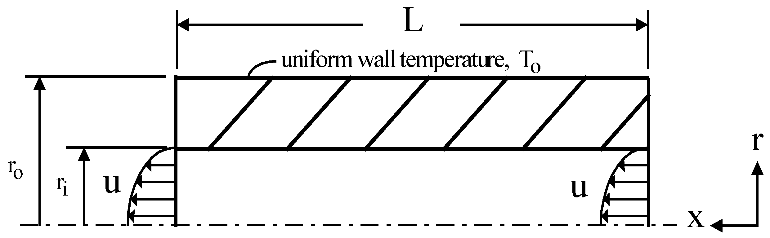
The flow situation in the present study is involved with an incompressible flow through a pipe, which is externally heated at different temperatures. The pipe is shown schematically in Figure 1. The flow field is assumed to be axisymmetric and a uniform outer wall temperature is assumed along the pipe length.

The equations governing the flow field are simplified after the consideration of Boussinesque approximations, in which case k-ε turbulence model can be used to account for the turbulence characteristics. In cylindrical polar coordinates the conservation equations are written as:

Continuity:

(1)

Momentum:

(2)

Energy:

(3)

where Pr and Pr_t are laminar and turbulent Prandtl numbers respectively.

In order to determine the turbulent viscosity and the Prandtl number, the k-ε turbulence model is used. The constitutive equations for the turbulent viscosity are as follows:

(4)

where k and ε are the turbulent kinetic energy generation and the dissipation variables respectively. The transport equation for k is:

(5)

where

(6)

The transport equation for ε is:

(7)

The generation of turbulence kinetic energy, ε and its dissipation at the inner wall of the pipe (r = r_i) is zero. The Prandtl numbers in transport equations of kinetic energy generation and dissipation are Pr_k and Pr_ε, respectively. The Prandtl number varies with Reynolds number [13]. The values in

Table 1. The turbulent Prandtl numbers and the resulting Nusselt numbers for the validation and the present study cases.

Laminar Reynolds Number (Re)	Turbulent Prandtl Numbers		Nusselt Number (Nu)		Abs. % Diff.
	Prt (k)	Prt (ε)	Reference No. (13)	Present Study
10000	0.097	0.097	80	77.5	3.1
30000	0.117	0.117	215	206	4.3
50000	0.128	0.128	338	341	0.9

are employed during the simulations, since each simulation is carried out for a fixed Reynolds number.

In order to minimize computer storage and run times, the dependent variables at the walls were linked to those at the first grid from the wall by equations, which are consistent with the logarithmic law of the wall. Consequently, the resultant velocity parallel to the wall in question and at a distance y₁ (where y⁺≤30) from it corresponding to the first grid node was assumed to be represented by the law of the wall equations [14], i.e.:

(8)

where, κ is a universal von-Karman constant and e is a universal turbulence parameters and their values are κ = 0.417 and e = 9.37, from which the wall shear stresses were obtained in solving the momentum equations. The constants used in the transport equations are [14]:

A radial step length of approximately two viscous sub-layer thickness (y⁺ = 5), where y⁺ = y [(τ_w/$\mathsf{\rho }$) ^1/2/(μ/$\mathsf{\rho }$)] is employed. In the axial and radial directions, the grid contains 64×300 nodes in the fluid region and 64×100 nodes in the solid region, employed to obtain the grid independent solution. The grid nodes are distributed to give a high concentration lines near the wall provided that the wall adjacent nodes are positioned at y⁺ ≈ 5. The grid independency tests were carried out by using the different grid nodes and the grid distribution tests were also conducted and based on the findings, the grids giving optimum solution is ensured as consistent with the early work [13]. The Nusselt number (Nu) predicted from the present study and the results of the previous study [13] are shown with Reynolds number in table 1. It can be observed from the table that the present predictions for Nu agree well with the previous results. However, small discrepancies are observed between both results at high Reynolds numbers. This may be due to slightly over predicting the turbulent kinetic energy generation at high Reynolds number by the turbulent model (k-ε model) introduced in the present study. However, this difference is small.

Since the fluid flow in the pipe and the external heating of the pipe take place at steady-state, the conduction in the solid is:

(9)

The boundary conditions:

The relevant boundary conditions for the conservative equations of flow and solid are:

1)

At pipe axis (r = 0):

2)

At inner solid wall (r = r_i):

No-slip conditions are considered, i.e.: u_w = 0 and v_w = 0

3)

At pipe inlet (x=0):

Uniform flow and uniform temperature were assumed.

4)

At pipe outlet (x=L):

All the gradients of the variables were set to zero, i.e.: ∂ϕ/∂η = 0

where φ is the fluid property and η is any arbitrary direction.

5)

At outer surface of the pipe (r = r₀):

Uniform surface temperature is assumed, i.e.: T = T₀ (K)

6)

At solid-fluid interface (r = r_i), i.e.:

Entropy Analysis

The irreversibility involved in the thermal system due to momentum and energy transport, results in continuous entropy production in the system. The local entropy generation per unit volume for an incompressible Newtonian flow system is [15]:

(10)

where the first term represents the entropy generation due to heat transfer while the second term is the entropy generated due to viscous dissipation in the flow system. In polar coordinates the viscous dissipation (Φ) can be written as:

(11)

where u is the axial velocity and v is the radial velocity.

Total entropy generation rate over the volume is:

(12)

and the rate or irreversibility is:

(13)

Eq. (10) is used to determine the volumetric entropy generation rate while Eq.(13) is used for the irreversibility rate.

Results and Discussion

Flow through a heated pipe and entropy generation in the flow system is presented for three outer wall temperatures (500 K, 750 K and 1000K) and three Reynolds numbers (10000, 30000 and 50000). The pipe used in the study is 4 meter long. For computer storage reasons, it is difficult to use longer pipes. To generate enough entropy in the pipe and to study the influence of temperature distribution in the pipe on entropy distribution, large values of pipe outer wall temperatures (in the range form 500 K to 1000 K) are used in the study. It should also be noted that the water temperature selected was excessive, which required pressurized water. The pipe diameter is taken as 0.08 meter and the pipe thickness as 0.024 meter. In this study, the temperature distribution in the pipe is presented in a non-dimensional form (T^*), which is calculated as:

(14)

where T_inlet is the pipe inlet temperature and T_mean is the mean temperature of all grid points.

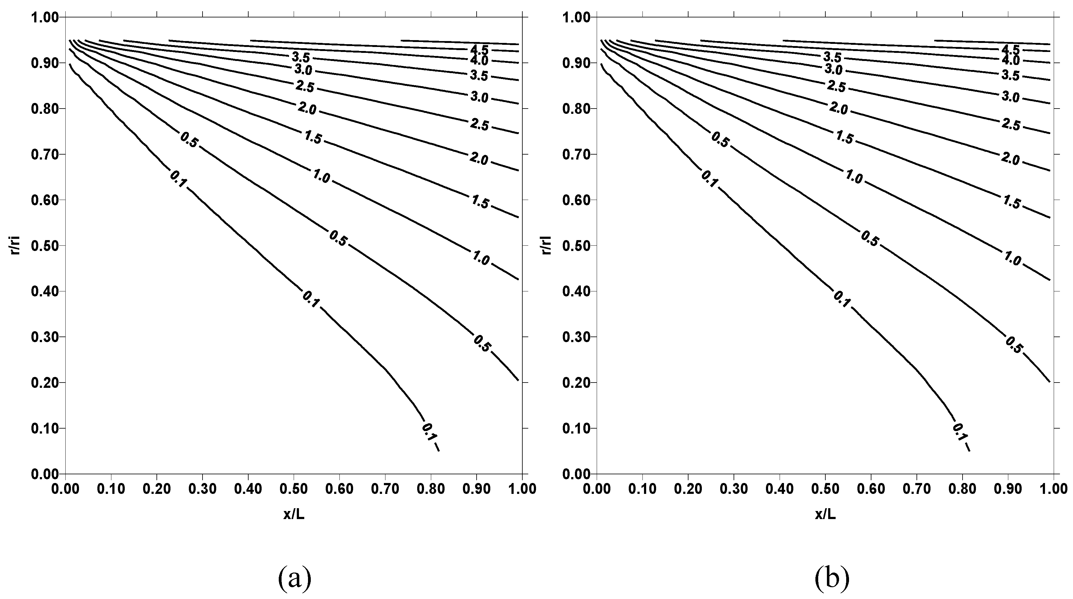
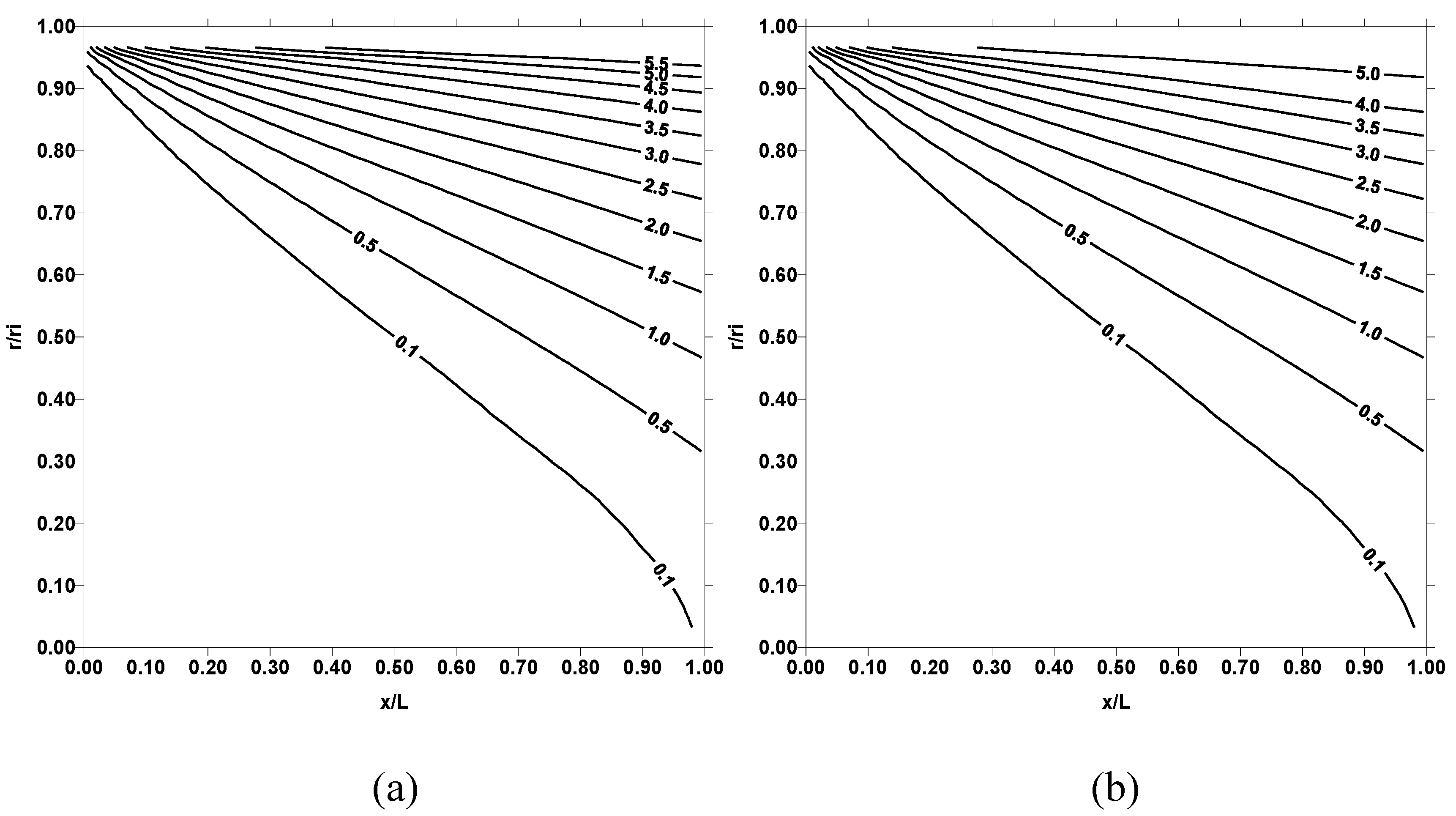
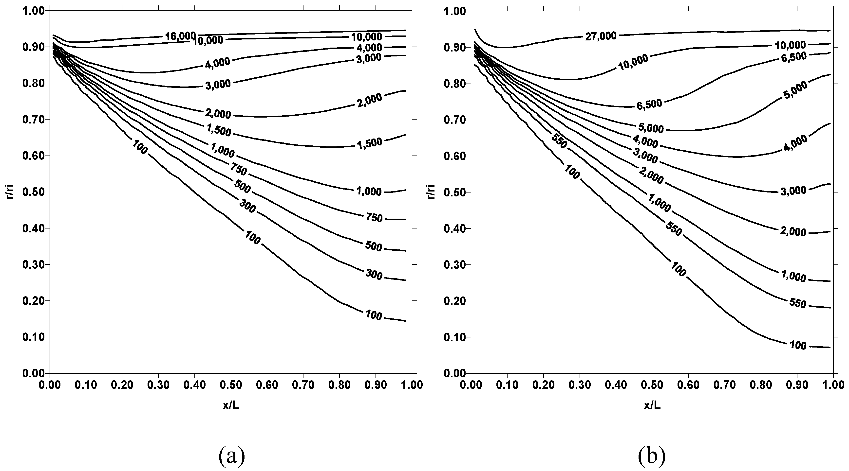
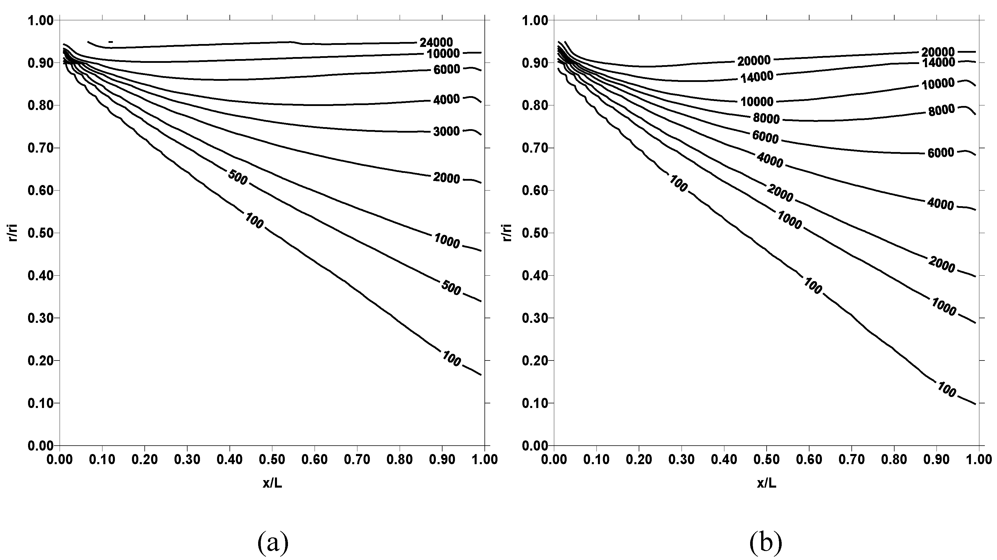
Figure 2 shows dimensionless temperature (T^*) contours in the fluid for two pipe wall temperatures and Reynolds number of 10000. Dimensionless temperature (T^*) contours show similar behavior for all the pipe wall temperatures employed (500 K and 1000 K). In general, at pipe inlet where x/L is less, dimensionless temperature attains low values. In this case, the fluid entering into the pipe does not have enough duration to gain thermal energy from the pipe wall. Consequently, constant temperature contour extends further inside the fluid in this region. As the pipe length extends, high temperature contours are developed in the region close to the pipe wall. This is because of the convective heating of the fluid in the vicinity of the pipe wall. In the case of entropy production, as seen from Figure 3, entropy contours do not follow the temperature contours. This is because of the entropy is proportional to the temperature gradient rather than temperature. When comparing the entropy contours obtained for 500 K and 1000K, the contours differ significantly in the two cases. This is more pronounced in the region close to the pipe wall. This is because of the losses due to fluid friction in the wall region as well as high fluid temperature gradient due to elevated wall temperature, which enhances heat transfer rates from the wall to fluid.

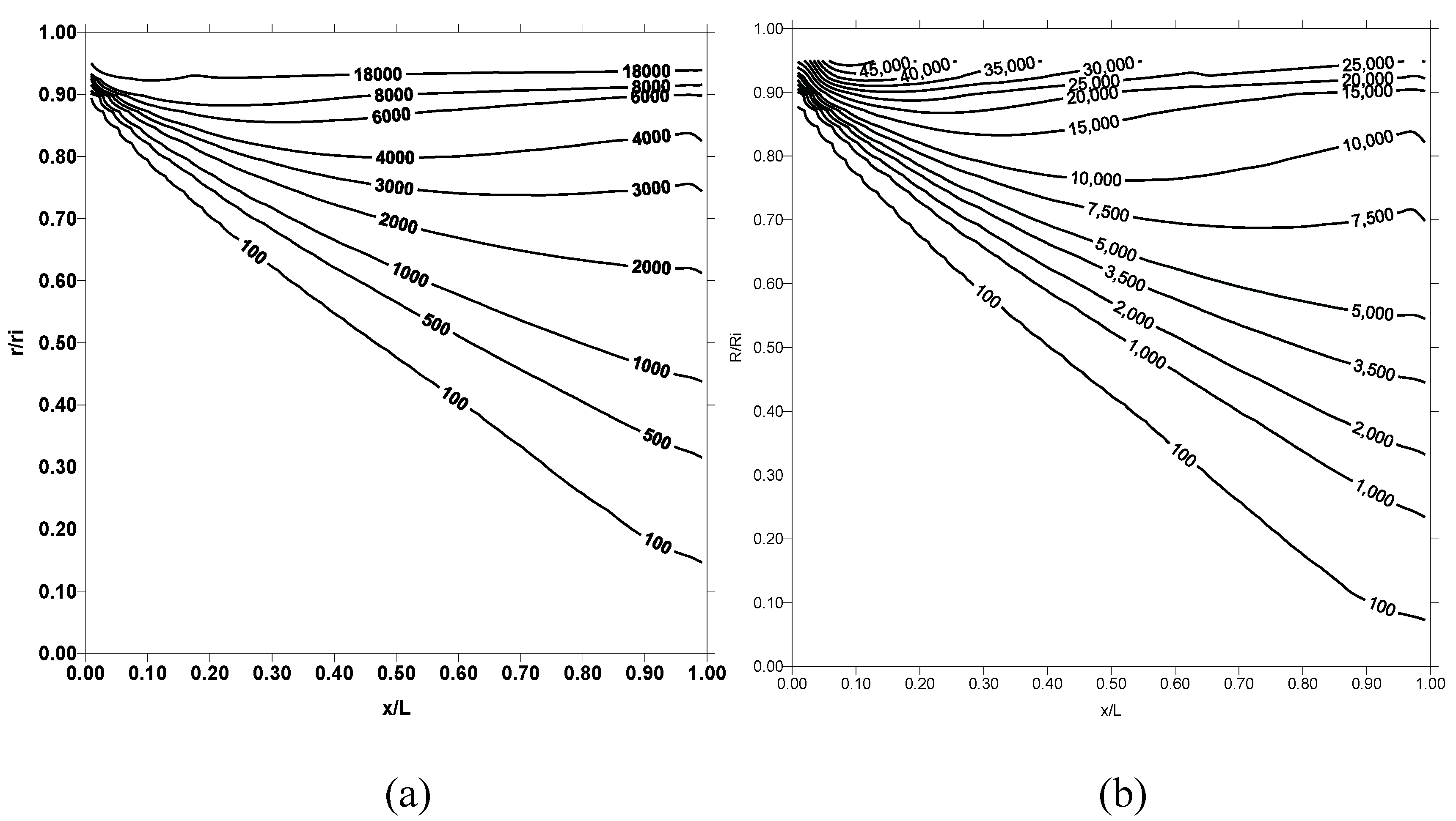
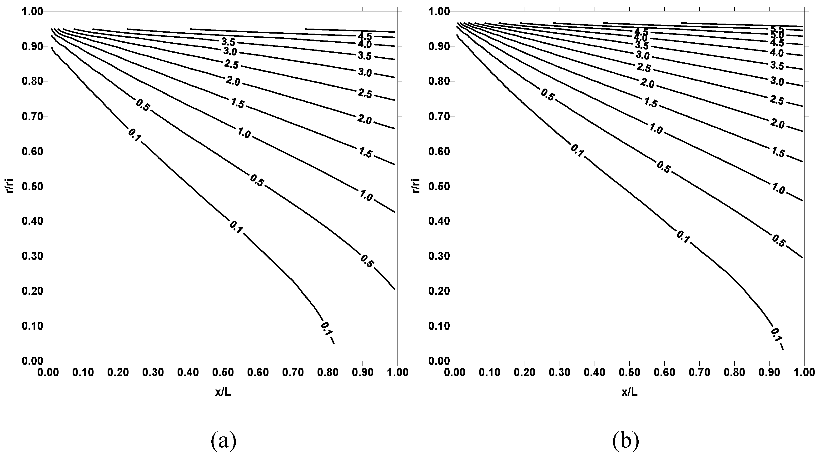
Figure 4 shows dimensionless temperature (T^*) contours for three pipe wall temperatures and Reynolds number of 30000, while Figure 5 shows corresponding entropy contours. Temperature contours behave similar to those obtained for Reynolds number 10000, provided that the magnitude of temperature contours in the surface region increases. This occurs because of the high convective heat transfer rates, which enhances with increasing Reynolds number. Entropy contours change for the Reynolds number 30000 as compared to their corresponding to 10000. This is more pronounced for pipe wall temperature 1000 K. It should be noted that the frictional losses due to viscous dissipation reduces as Reynolds number increases for the turbulent flow. Despite this fact, entropy contours attain high values for Reynolds number of 30000. This is because of the entropy generation due to heat transfer rates, which improve considerably at high Reynolds number.

Figure 6 shows dimensionless temperature (T^*) contours for three outer wall temperatures and Reynolds numbers of 50000, while Figure 7 shows corresponding entropy contours. Temperature contours in the vicinity of the pipe wall increases further as compared to those shown in Figure 4 because of the high convective heat transfer rates from the pipe wall to fluid. Entropy contours differ significantly from those presented in Figure 3 and Figure 5, particularly for temperature 1000 K. Consequently, increasing Reynolds number and pipe wall temperature enhances the heat transfer rates, which in turn results in high rate of entropy production.

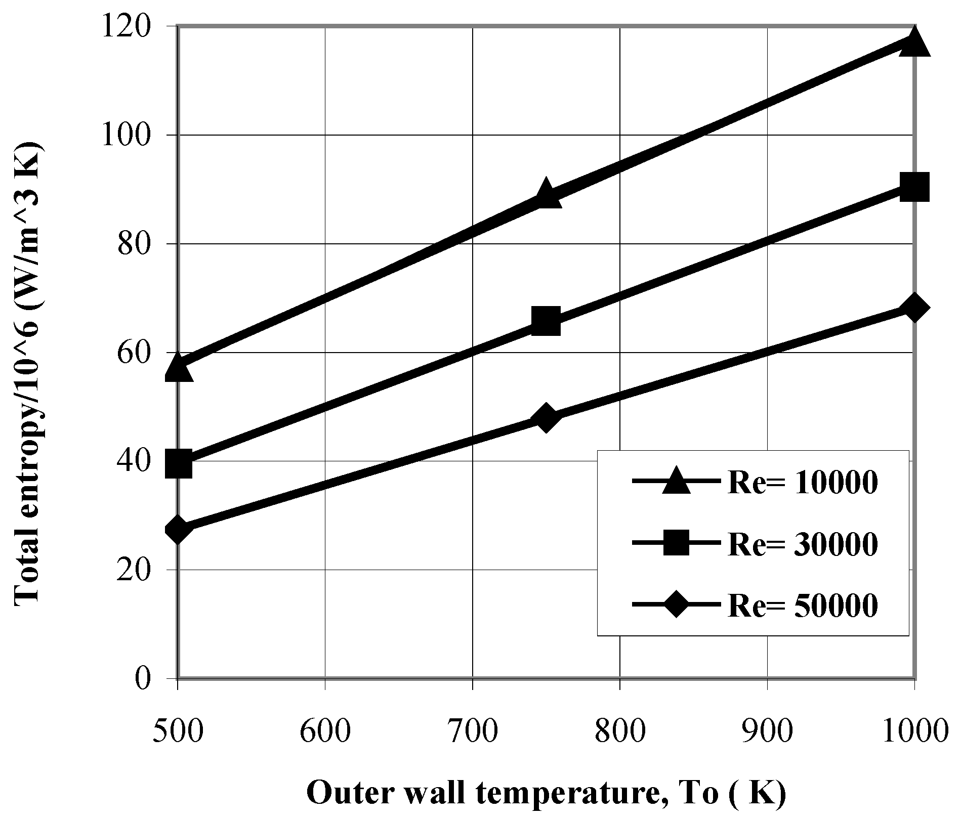
Figure 8 shows total entropy rate produced in the fluid system with wall temperature as Reynolds number is variable. Entropy production rate increases considerably with increasing pipe wall temperature and Reynolds number. This situation indicates that entropy generation due to heat transfer dominates over its counterpart corresponding to fluid friction. This is because of increasing Reynolds number in turbulent flow lowers the frictional losses; therefore, the entropy production rate is lowered. Consequently, increasing entropy production rate at high Reynolds number is because of heat transfer process only. It can be observed from Figure 8 that entropy generation can be minimized by reducing the pipe wall temperature, while increasing the Reynolds number.

Conclusions

Heat transfer and entropy analysis for flow through pipe system are carried out. A numerical method using a control volume approach is employed in the computations. Steel pipe is selected as pipe material, while water is considered as fluid. The simulations are repeated for three Reynolds numbers and three pipe wall temperatures. It is found that entropy contours do not follow the temperature profiles. Entropy production rate is low at the pipe inlet and as the pipe length increases it signifies. Moreover, entropy production rate is high in the region close to the pipe wall, which is more pronounced for high wall temperature. This is because of high temperature gradient in this region. Increasing Reynolds number enhances the entropy production rate. This is because of the enhanced heat transfer rates, i.e. convective heating of the fluid enhances at high Reynolds number. This indicates that entropy production due to heat transfer dominates over the entropy production due to fluid friction, since frictional losses reduce with increasing Reynolds number in the pipe flow.