Since the metric signature is not a continuous variable its dynamics can not be described by differential equations. To see this consider the multi-dimensional metric.
is the signature of the metric with viel-bein indices
= 0, 1, 2, 3, 5, 6,···.
xA are the coordinates on the total space of the principal bundle with a structural group
, and
C, D are the multidimensional (MD) coordinate indices. The metric on the total space of the principal bundle (we will consider gravity on the principal bundle) can be rewritten
,
are the viel-bein indices for the fibre of the principal bundle, and
c, d are the coordinate indices on the fibre;
,
and
α, β play the same role for the 4D base of the principal bundle. For the continuous quantities,
, we have gravitational equations, but
are discrete (non-differentiable) quantities without dynamical equations. Thus the dynamics of the metric signature,
, can not be described by differential equations. We will instead apply a quantum-like description for these degrees of freedom. This description will be stochastic along the general lines of ’t Hooft’s proposition that quantum gravity may be a stochastic phenomenon [
7]. The gravitational field equations on the principal bundle are deduced in
Appendix (A). In the following subsection (4.1) we take Λ
1,2 = 0.
4.1 The 5D Fluctuating Universe
In this subsection we consider the scenario where at the origin of the Universe a fluctuation between Euclidean and Lorentzian metrics occurs. This is a modification of an idea initially proposed by Hawking where there may be regions of the Universe with Euclidean or Lorentzian signatures. The boundary between these two regions represents some quantum fluctuation between the different metric signatures. Such transitions between metric signatures could occur in the very Early Universe on the scale of Planck length.
We start with a vacuum 5D Universe with the metric
here
σ = ±1 for the Euclidean and Lorentzian signatures respectively. The 3D space metric
describes the Hopf bundle with an
S1 fibre over an
S2 base. In the 5-bein formalism we have
here
,
are the 5-bein indices and
According to the following theorem [
4]
Let G be a structural group of the principal bundle. Then there is a one-to-one correspondence between the G-invariant metricson the total space and the triples .
Here gµν is the 4D metric on the base; are the gauge fields of the group G (the off-diagonal components of the multidimensional metric); dl2 =
σaσa is the symmetric metric on the fibre a = 5, ··· , dim
G is the index on the fibre and µ = 0, 1, 2, 3
is the index on the base. the metric in Eq. (16) has the following electromagnetic potential
For this potential the Maxwell tensor is
which yields an electrical field like
and a magnetic field like
The 5D, vacuum Einstein equations [
6] resulting from Eq. (16) are
where
is the Einstein tensor. Our basic assumption is that
at the Planck scale there can exist regions where a quantum fluctuation between Euclidean and Lorentzian metric signatures occurs. There are two copies of the classical equations (24): one with
σ = +1 and another with
σ = −1. It is this quantity σ which we take as having quantum fluctuations between its two discrete values. The basic question under this assumption is how to calculate the relative probability for each pair of equations from (24) (the ones with
σ = +1 versus the ones with
σ = −1).
We will define the probability for each pair of equations in terms of the algorithmic complexity of each pair. We can diagrammatically represent the fluctuations between the Euclidean and Lorentzian versions of Einstein’s equations in the following way
The signs ± indicates if the equation belongs to the Euclidean or Lorentzian mode. Expression (25) sums up the idea that treating
σ as a quantum quantity leads to quantum fluctuations between the classical equations:
or
. The probability connected with each pair of equations (
or
)
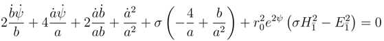
is determined by the AC of each equation. The
equation in the Euclidean and Lorentzian modes is respectively
Let us consider the
ψ = 0 case (below we will see that this is consistent with the
equation). It is easy to see that Eq. (26a) can be deduced from the instanton condition
The second equation (26b) does not have a similar simplification via the instanton condition (27). This is just the well known fact that instantons can exist only in Euclidean space. Based of this simplification from a second order equation (26a) to a first order equation (27) we consider the Euclidean equation (26a) simpler from an algorithmic point of view than the Lorentzian equation (26b). To a first, rough approximation we can take the probability of the Euclidean mode as
and for the Lorentzian mode as
. Strictly the exact definition for each
is
where
is the AC for the
or
equation. For
we have
and
.
The expression for the probability in Eq. (28) can be seen as the discrete variable analog of the Euclidean path integral transition probability. For a continuous variable the Euclidean path integral gives the probability for the variable to evolve from some initial configuration to some final configuration as being proportional to the exponential of minus the action (∝ e−S). Eq. (28) is similar, but with the AC replacing the action. The denominator normalizes the probability (it is a sum rather than integral since we are dealing with a discrete variable).
The
equation in the Euclidean and Lorentzian modes is respectively
The Lorentzian mode (29b) has a trivial solution
provided the instanton condition (
i.e. ) holds. Thus for this equation we take the Lorentzian mode as having a smaller AC, and in the contrast with the previous subsection, the Lorentzian mode has the greater probability. Again to a first, rough approximation the probability of the Euclidean mode is
and consequently for the Lorentzian mode
.
Taking into account (30) we can write these equations as
For the Euclidean mode (
σ = +1) with the instanton condition (27)) one can have
b =
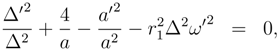
a (an isotropic Universe) which reduces the two equations of (31) to
only one equation
For the Lorentzian mode
(an anisotropic Universe) there are still two equations
Thus under the instanton condition (27) and ψ = 0 we find that the Euclidean mode (32) effectively reduces to one, second order equation which corresponds to an isotropic Universe; the Lorentzian mode (33) still has two, second order equations which describe an anisotropic Universe. Thus we assign the Euclidean mode the smaller AC and as for the previous equations make the rough approximation for the Euclidean mode, for the Lorentzian mode.
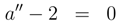
The equation
has the following form
Assuming all the previous conditions (the instanton condition,
ψ = 0, and
b =
a) the Euclidean mode equations become
while the Lorentzian mode equations become
The instanton condition again implies that the Euclidean mode has a smaller AC. Thus to a first, rough approximation we take
and
.
Mixed system of the equations Under the approximation where the probability associated with each of the equations in (24) is
p ≈ 0 or 1 the
mixed system of equations which describe a Universe
fluctuating between Euclidean and Lorentzian modes
here
b =
a,
ψ = 0 and the instanton condition are all assumed to hold. This system of mixed Euclidean and Lorentzian equations has the following simple solution
The mixed origin of the Universe The following model for the quantum birth of Universe has been advanced by Hawking : one begins with an Euclidean space of the Planck size (R4, S4 or some other smooth non-singular Euclidean space); then a Lorentzian Universe emerges from a boundary of this initial Euclidean piece. In this scenario the Euclidean and Lorentzian spaces are connected by a hypersurface with a mixed signature.
In this section we present a variation of this picture for the quantum mechanical origin of the Universe. We assume that the Universe begins as a quantum fluctuating system between Euclidean and Lorentzian modes. Then at some point in time there is a quantum transition to the Lorentzian mode.
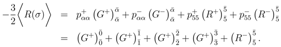
To support these statements mathematically we begin by calculating the average of the Ricci scalar
where
p+ and
p− are the probabilities for the scalar curvature with
σ = +1 and
σ = −1 respectively. Using
and averaging gives
Thus for the mixed system of equations we find
In this toy model the Universe originates from an empty, multidimensional, non-singular (in the sense that
), spacetime of Planck scale size (
τ τPl). In our model the spacetime is
M4 ×
S1, with
M4 being a space with fluctuating metric signature: Euclidean ↔ Lorentzian. At some point a quantum transition to the Lorentzian mode occurs, and at the same or later time the 55 component of the metric becomes a non-dynamical quantity. Thus the fluctuation of the metric signature of the original Planck scaled, 5D Universe leads to a 4D Lorentzian Universe
and a “frozen” or non-dynamical 5
th dimension.
4.2 The 7D Fluctuating Universe
In this subsection we study a 7D cosmological solution with a fluctuating metric signature as in the last subsection. We take the gauge group of the EDs as
=
SU(2), with the 7D metric taking the form
Most of the calculational details for this 7D metric are given in
Appendix (A).
The total space of the principal bundle is denoted as
E; the structural group is denoted as
. The factor-space
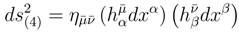
is the base of the principal bundle, and is described by the 4D metric
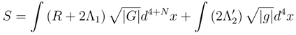
which is the last term in Eq. (43). We now insert a 4D cosmological constant term into the MD action
R is the Ricci scalar and
![]()
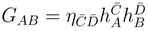
is the MD metric on the total space;
![]()
is the 4D metric on the base of the principal bundle;
![]()
is the metric on
;
G, g and
γ are the appropriate metric determinates; Λ
1,2 are the MD and 4D Λ-constants;
. The MD action of Eq. (45) has several points in common with the 4D EYM action considered in Ref. [
17] (non-zero cosmological constants and effective SU(2) “Yang-Mills” gauge fields). Eq. (45) also has a connection to the action for the Non-gravitating Vacuum Energy Theory [
18]. In Ref. [
18] Guendelman considers an action which has degrees of freedom which are independent of the metric, with the resulting action having two measures of integration (involving metric and nonmetric degrees of freedom). Eq. 45 incorporates two distinct degrees of freedom : the continuous variables,
, and the discrete variables,
. In Ref. [
18] both the metric and non-metric degrees of freedom were continuous.
The independent,
continuous degrees of freedom are: the vier-bein
, the gauge potential
and the scalar field
b(
xα).
is defined as
xb are the coordinates on the group
;
are the 1-forms satisfying
are the structural constants of SU(2). Varying the action in Eq. (45) with respect to
,
and
b leads to (see the
Appendix for details)
Eq. (48a) are the Einstein vacuum equations with Λ-terms; Eq. (48b) are the “Yang-Mills” equations; Eq. (48c)is reminiscent of Brans-Dicke theory since the metric on each fibre is symmetric and has only one degree of freedom - the scalar factor
b(
xµ).
We now investigate Eqs. (48a)-(48c) using the ansatz
σ = ±1 describes the possible quantum fluctuation of the metric signature between Euclidean and Lorentzian modes,
are SU(2) gauge potentials,
is the metric on the unit
S3 sphere and
x0 =
t, x1 =
χ, x2 =
θ, x3 =
φ, x5 =
α, x6 =
β, x7 =
γ. (
α, β, γ are the Euler angles for the SU(2) group)
The off-diagonal components of the MD metric take the instanton-like form [
19] [
20]
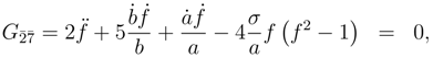
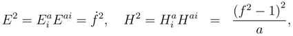
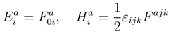
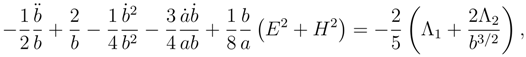
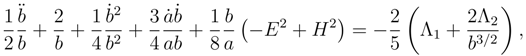
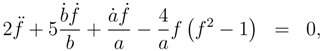
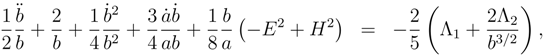
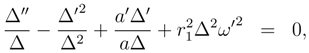
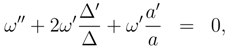
Substituting into Eqs. (48a)-(48c) gives
;
i = 1, 2, 3 are space indices; the “electromagnetic” fields are
is the field strength tensor for the non-Abelian gauge group. The wormhole instanton of Ref. [
17] had a vanishing “electric” field. In contrast the solution studied here has both non-vanishing “electric” and “magnetic” fields.
As in the 5D case we assume a quantum fluctuation between Euclidean and Lorentzian modes which can be described by a diagram similar to Eq. (25))
As in the 5D case we will estimate the probability for each pair of equations in (54).
This equation in the Euclidean mode is
which has the instanton solution
where
Eq. (56) implies the instanton condition
In the Lorentzian mode
and the instanton solution (58) is not a solution of (59), since the non-singular, instanton solution exists only in the Euclidean case. Thus in terms of the AC criteria the Euclidean equation (55) is simpler than Lorentzian equation (59), since it is equivalent to the first order differential equation (56).
To a first, rough approximation we set the probability of the equation for the Euclidean mode to and the Lorentzian mode to . The exact definition for each probability is given in Eq. (28). If we have and .
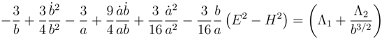
This equation in the Euclidean and Lorentzian modes is respectively
The Lorentzian mode equation is simpler because the two last terms annihilate as a consequence of the instanton condition (58). To a first rough approximation we set the probability of the
equation for the Euclidean mode to
and the Lorentzian mode to
.
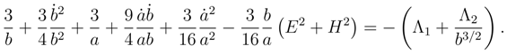
This equation in the Euclidean mode and Lorentzian mode is respectively
In this case because of the instanton condition (58) the Euclidean equation is simpler and therefore in the first rough approximation we can set the probability of the
equation for the Euclidean mode to
and the Lorentzian mode to
.
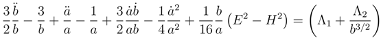
This equation in the Euclidean mode and Lorentzian mode is respectively
As in the previous paragraph, as a consequence of the instanton condition (58), the Euclidean mode is simpler. Therefore in the first rough approximation we set
and
.
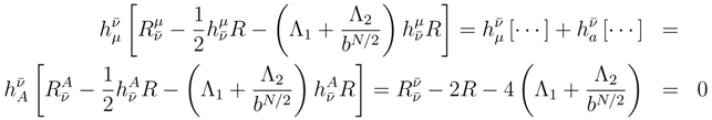
Mixed system of equations The mixed system of equations for the 7D spacetime with fluc-tuating metric signature is
The solution for this system is
The existence of this solution is somewhat surprising ! Normally in any dimension the Bianchi identities are satisfied. Therefore some gravitational field equations are not independent of the others. Ordinarily the superfluous equations are associated with initial conditions (i.e. Eq. (63c) above). In our case the mixed system above comes from a model with a varying metric signature. As a consequence the Bianchi identities are not correct and this system should be unsolvable. Evidently the solution is a condition for the solvability of the mixed system which uniquely defines the Λ-constants. If the solution in Eqs. (64) is unique then it must be absolutely stable.
The physical meaning of this solution is:
Eq. (64a) implies a flat 4D Einstein spacetime that is not effected by matter.
Eq. (64b) implies a Polyakov - ’t Hooft instanton gauge field configuration which is not effected by gravity.
Eq. (64c) implies a frozen ED.
Eqs. (64d)-(64e) imply that the dynamical equations uniquely determine the Λ1,2-constants.
It is interesting to note that the effective cosmological constant terms on the right hand side of Eqs. (48a) (48c) (
i.e. Λ
1 and Λ
2/b3/2) are inversely proportional to the size of the ED,
b0. Thus in order to have a small cosmological constant term one needs to have a large ED. This could be seen as supporting the large extra dimensions scenarios [
14].


 is the MD metric on the total space;
 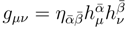 is the 4D metric on the base of the principal bundle;
 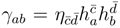 is the metric on ; G, g and γ are the appropriate metric determinates; Λ1,2 are the MD and 4D Λ-constants; . The MD action of Eq. (45) has several points in common with the 4D EYM action considered in Ref. [17] (non-zero cosmological constants and effective SU(2) “Yang-Mills” gauge fields). Eq. (45) also has a connection to the action for the Non-gravitating Vacuum Energy Theory [18]. In Ref. [18] Guendelman considers an action which has degrees of freedom which are independent of the metric, with the resulting action having two measures of integration (involving metric and nonmetric degrees of freedom). Eq. 45 incorporates two distinct degrees of freedom : the continuous variables, , and the discrete variables, . In Ref. [18] both the metric and non-metric degrees of freedom were continuous.