Article

New Modified Generalized Inverted Exponential Distribution and Its Applications

by
Zakeia A. Al-Saiary
1,* and
Hana H. Al-Jammaz
1,2
1
Department of Mathematics and Statistics, College of Science, University of Jeddah, Jeddah 22254, Saudi Arabia
2
Department of Statistics and Operations Research, College of Science, Qassim University, Buraydah 51482, Saudi Arabia
*
Author to whom correspondence should be addressed.
Entropy 2026, 28(2), 161; https://doi.org/10.3390/e28020161
Submission received: 2 December 2025 / Revised: 19 January 2026 / Accepted: 26 January 2026 / Published: 31 January 2026
(This article belongs to the Special Issue Statistical Inference: Theory and Methods)

Abstract

In this paper, a statistical model with three parameters is proposed which is called New Modified Generalized Inverted Exponential Distribution (MGIE). In addition, several statistical characteristics of the MGIE distribution are obtained, including quantile function, median, moments, mode, mean deviation, harmonic mean, reliability, hazard and odds functions and Rényi entropy. Moreover, the estimators of parameters are found using the maximum likelihood estimation method. A simulation study using the Monte Carlo method is performed to assess the behavior of the parameters. Finally, three real data sets are applied to demonstrate the importance of the proposed distribution.

1. Introduction

Given the data revolution and its importance in the modern era, and because traditional distributions cannot accurately represent the behavior of many data sets across various fields, statistical researchers have resorted to generat new distributions by creating families in order to provide greater flexibility and relevance. This highlights the importance of the widespread adoption of these families.
There are several examples of these families. A novel class of exponentiated generalized distributions was introduced by [1]. Type II power Topp–Leone-G family was proposed by [2]. The Lomax-G was generated by [3]. In 2020, a novel class of heavy-tailed distributions, which is referred to as a new extended family of heavy-tailed distribution, was found by [4]. A new Modified-X family was derived by [5]. The BurrXII-log-logistic family was introduced by [6]. In 2022, A new modified-G (NModi-G) family, utilizing a new statistical technique, was studied by [7]. Based on the previous group, we established our new modified model.
The cumulative distribution function (CDF) of the NModi-G family is given by
G ( x ; σ , ϕ ) = F ( x ; ϕ ) σ [ σ 1 + F ( x ; ϕ ) ] ,
where σ 1 , σ 1 , x R , and F ( x ; ϕ ) is a baseline CDF and ϕ represents the parameters of the baseline distribution.
The probability density function (PDF) of (1) is given by
g ( x ; σ , ϕ ) = f ( x ; ϕ ) σ [ σ 1 + 2 F ( x ; ϕ ) ] .
Recently, many statisticians have shown interest in generalized inverted exponential distribution (GIED), which was introduced by [8]. For example, Topp–Leone generalized inverted exponential distribution (TLGIE) [9], type II Topp–Leone generalized inverted exponential distribution (TIITLGIE) [10]. Various approaches were discussed to find estimates of the shape and scale parameters by [11]. A new model of bivariate exponentiated generalized inverted exponential distribution was proposed by [12], and parameters were estimated when the data involved were censored samples of the first type by [13].
The GIED has the following PDF:
f ( x ) = ( θ λ x 2 ) e λ x [ 1 e λ x ] θ 1 , x > 0 , λ , θ > 0 ,
and the CDF is given by:
F ( x ) = 1 [ 1 e λ x ] θ , x > 0 , λ , θ > 0 ,
where θ is a shape parameter and λ is a scale parameter.
Although our model is based on the general framework of the NModi-G model family, it introduces specific modifications that were not found in previous work by depending on generalized inverted exponential distribution as a baseline. In particular, it provided better flexibility and suitability when we added the proposed distribution compared to other families, such as the exponential family and the Topp–Leone family. This is clearly demonstrated through applications on real data.
We chose the generalized inverted exponential (GIE) distribution as the baseline because of its diverse risk function shapes, which support a wide range of risk profiles. It also provides heavier tails and greater flexibility than the standard inverted exponential and demonstrated strong experimental performance in lifetime data modeling. These features make it a suitable and efficient baseline for developing the proposed model.
The rest of this paper is organized into the following sections. In Section 2, the PDF and CDF of MGIE will be presented. In addition, the major statistical properties of our model, such as the quantile function, moments, reliability function, hazard function, mean, median, and mode can be found in Section 3. Furthermore, Rényi entropy is derived in Section 4. In Section 5, we estimate the parameters of the model. Also, we perform a simulation study in Section 6. Finally, bio-sciences data sets are applied in Section 7. These data sets were primarily chosen because they are widely used in the evaluation of new statistical models and provide suitable data characteristics for testing the statistical performance of the proposed distribution. Also, the basic family from which the proposed distribution originated was designed to fit this type of data, as mentioned in [7].

2. The Modified Generalized Inverted Exponential Distribution

In this section, we introduce modified generalized inverted exponential distribution which contains three parameters ( θ , λ , σ ) . The PDF and CDF of MGIE distribution is obtained by substituting Equations (3) and (4) in Equations (1) and (2):
g ( x ) = ( θ λ x 2 ) e λ x ( 1 e λ x ) θ 1 ( 1 + 1 σ 2 σ ( 1 e λ x ) θ ) ,
and
G ( x ) = 1 ( 1 e λ x ) θ ( 1 σ + 1 1 σ ( 1 e λ x ) θ ) ,
where θ is a shape parameter and λ , σ are scale parameters.
Using the following series:
( 1 x ) n = i = 0 n n i ( 1 ) i ( x ) i ( 1 ) n i ,
we can reformat PDF and CDF as follows:
g ( x ) = ψ 1 ( x ) 2 e λ x ( i + 1 ) + ψ 2 ( x ) 2 e λ x ( j + 1 ) ,
where
ψ 1 ( i , θ , λ , σ ) = ( 1 + 1 σ ) ( θ λ ) i = 0 θ 1 i ( 1 ) i ,
ψ 2 ( j , θ , λ , σ ) = ( 2 σ ) ( θ λ ) j = 0 2 θ 1 j ( 1 ) j ,
and
G ( x ) = 1 [ ζ 1 e λ x i ζ 2 e λ x j ] ,
where
ζ 1 ( i , θ , σ ) = ( 1 σ + 1 ) i = 0 θ i ( 1 ) i ,
ζ 2 ( j , θ , σ ) = ( 1 σ ) j = 0 2 θ j ( 1 ) j .
These formulas that involve infinite series allow for an accurate representation of the theoretical properties of the proposed distribution and are also common in the literature on generated distributions. From a practical standpoint, these expressions can be efficiently evaluated numerically using available statistical packages like R and Mathematica.

Some Ideal Sub Models as Special Cases from the Proposed Distribution

  • For θ = 1 , the proposed distribution in (5) transforms to Modified Inverse Exponential distribution (MIE) and it is given as follows:
    g ( x ) = λ x 2 e λ x ( 1 1 σ + 2 σ e λ x ) .
  • For θ = 1 and λ = 1 , the proposed distribution transforms to Modified Standard Inverse Exponential distribution (MSIE) and it is given as
    g ( x ) = 1 x 2 e 1 x ( 1 1 σ + 2 σ e 1 x ) .
  • For λ = 1 , the proposed distribution transforms to Modified Generalized Standard Inverse Exponential distribution (MGSIE) and it is given as
    g ( x ) = θ x 2 e 1 x ( 1 e 1 x ) θ 1 ( 1 + 1 σ 2 σ ( 1 e 1 x ) θ ) .
  • For σ = , the proposed distribution transforms to Generalized Inverted Exponential distribution (GIED) and it is given as
    g ( x ) = ( θ λ x 2 ) e λ x ( 1 e λ x ) θ 1 .
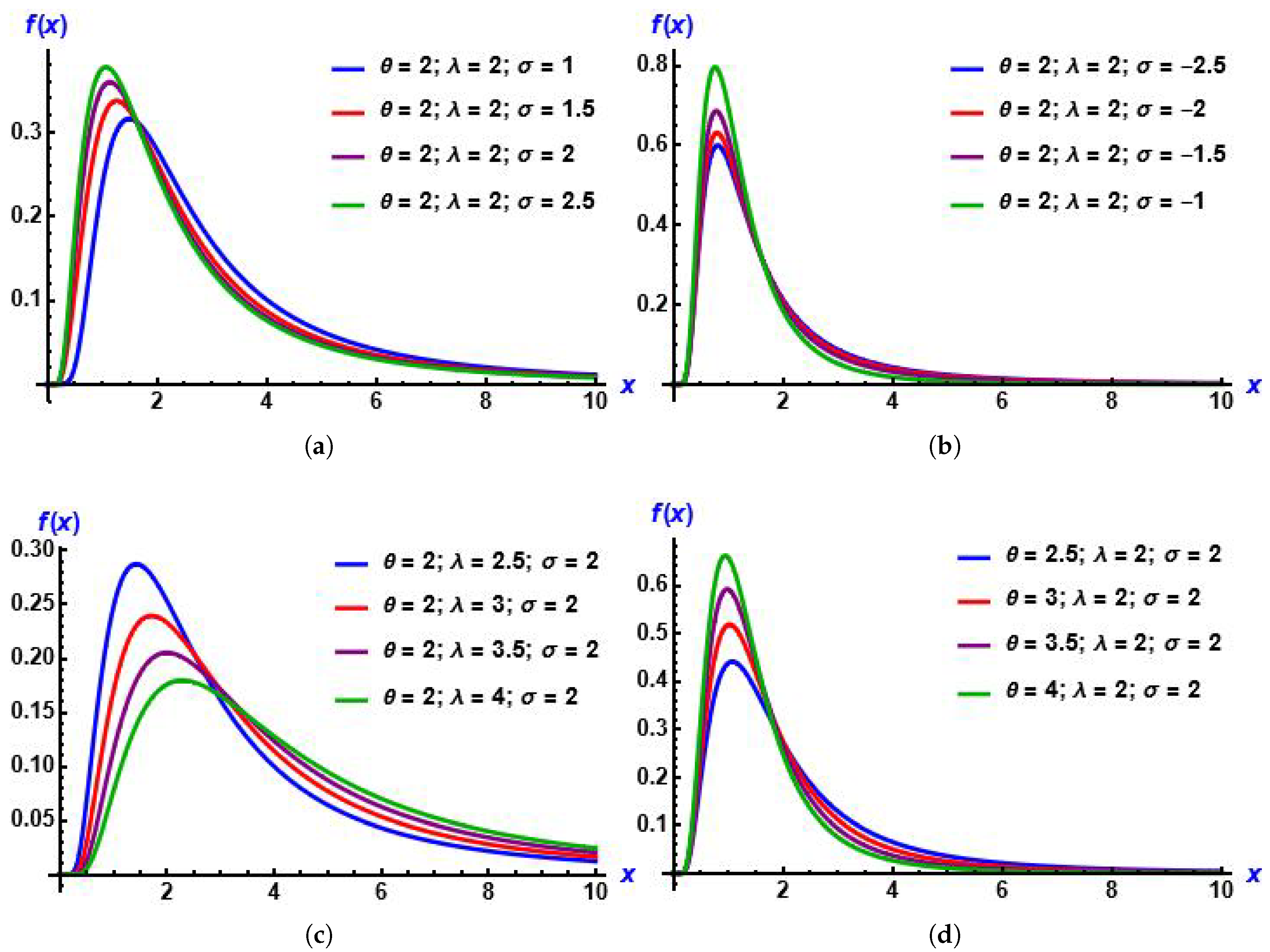
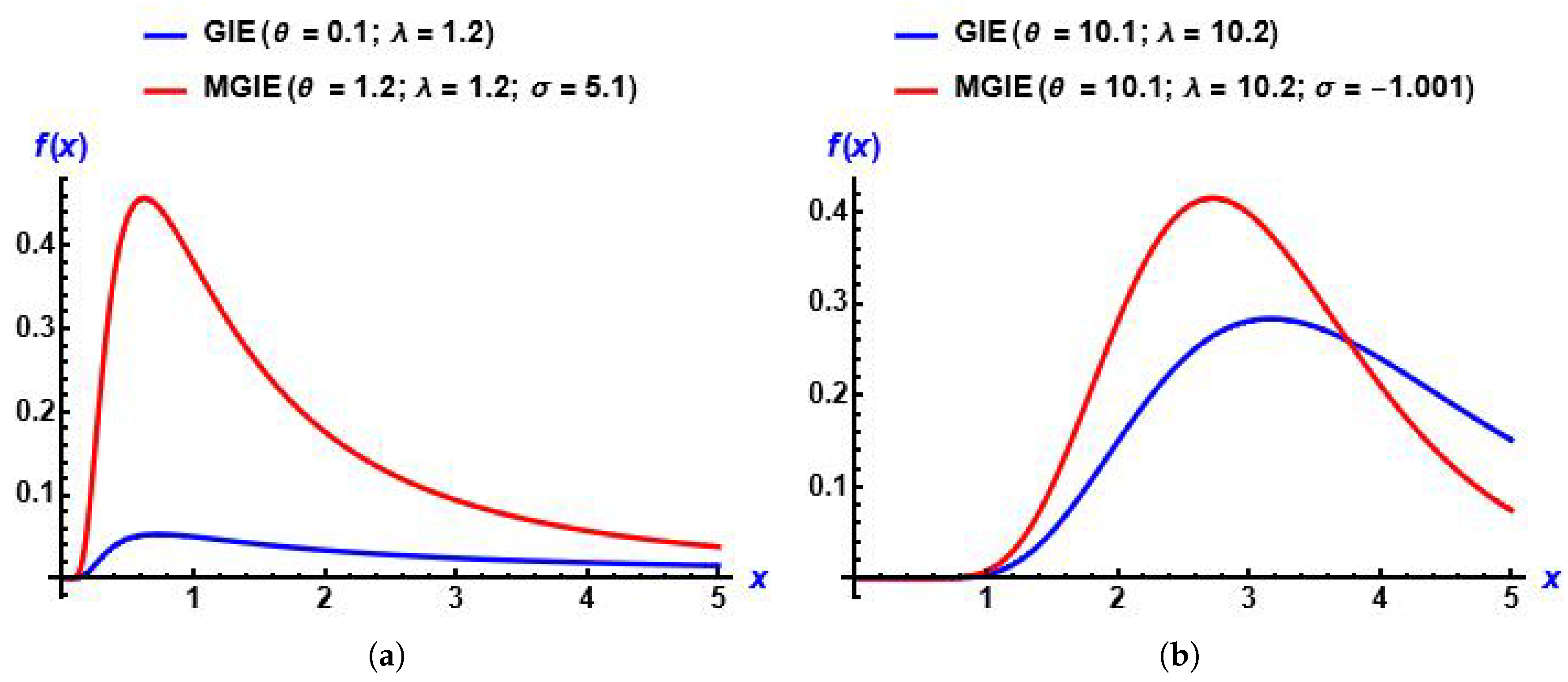
From plots in Figure 1, we can see that the MGIE distribution is skewed to the right and unimodal. Also, Figure 2 shows the effect of the added parameter on the baseline distribution.

3. Properties of MGIE Distribution

3.1. Quantile and Median

We can get the quantile function as follows:
x = Q ( u ) = G 1 ( u ) = F 1 ( k ) ,
where k is the solution of ( σ 1 ) k + k 2 σ u . See [5]
The quantile function of the MGIE distribution is given by
Q ( u ) = λ L o g [ ( 1 ( 1 1 2 ( 1 σ + 1 2 σ + 4 u σ + σ 2 ) ) 1 θ ) ] .
By putting U = 0.5 in the previous equation, we deduce the median of the MGIE distribution as
m = λ L o g [ ( 1 ( 1 1 2 ( 1 σ + 1 2 σ + 4 ( 0.5 ) σ + σ 2 ) ) 1 θ ) ] .

3.2. The r t h Moment

To find the r t h moment for x which has the MGIE distribution, we use the following equation:
μ r ´ = E ( x r ) = x r g ( x ) d x ,
by substituting Equation (7) in the previous equation:
μ r ´ = 0 x r [ ψ 1 ( x ) 2 e λ x ( i + 1 ) + ψ 2 ( x ) 2 e λ x ( j + 1 ) ] d x ,
where ψ 1 , ψ 2 are given in Equations (8) and (9), respectively.
Let
u = λ x ( i + 1 ) , w = λ x ( j + 1 ) ,
therefore, we get the r t h Moment of the MGIE distribution:
μ r ´ = [ ( ψ 1 ( λ ) r 1 ( i + 1 ) r 1 ( n = 0 ( 1 ) n ( n r + 1 ) n ! + E r ( 1 ) ) ] + [ ( ψ 2 ( λ ) r 1 ( j + 1 ) r 1 ( n = 0 ( 1 ) n ( n r + 1 ) n ! + E r ( 1 ) ) ] , n > r 1 ,
note that the E r ( 1 ) is generalized exponential integral [9]. It is given by
E n ( z ) = 1 e z t t n d t ,
and ψ 1 , ψ 2 are given in Equations (8) and (9), respectively.
Furthermore, we can find the mean of the MGIE distribution by equating r to 1:
μ = [ ( ψ 1 ( n = 0 ( 1 ) n n n ! + E 1 ( 1 ) ) ] + [ ( ψ 2 ( n = 0 ( 1 ) n n n ! + E 1 ( 1 ) ) ] ,
by substituting Equation (20) in the following formula:
M x ( t ) = r = 0 t r r ! E ( x r ) ,
we obtain the moment generating function (MGF) of the MGIE distribution:
M x ( t ) = r = 0 t r r ! [ ( ψ 1 ( λ ) r 1 ( i + 1 ) r 1 ( n = 0 ( 1 ) n ( n r + 1 ) n ! + E r ( 1 ) ) ] + [ ( ψ 2 ( λ ) r 1 ( j + 1 ) r 1 ( n = 0 ( 1 ) n ( n r + 1 ) n ! + E r ( 1 ) ) ] , n > r 1 .

3.3. Skewness and Kurtosis

The skewness and kurtosis are important statistical measures. Bowley’s coefficient of skewness is also known as quartile skewness [14] and it is given by:
B = Q ( 3 4 ) 2 Q ( 1 2 ) + Q ( 1 4 ) Q ( 3 4 ) Q ( 1 4 ) .
We can derive Moors’ coefficient of kurtosis by using octileis [15], which separate the dataset into evenly sized divisions. It has the following formula:
M = Q ( 7 8 ) Q ( 5 8 ) + Q ( 3 8 ) Q ( 1 8 ) Q ( 6 8 ) Q ( 2 8 ) ,
where Q(.) is given in (18).

3.4. Reliability Function

The reliability function is familiar as a survival function. It is used to determine the probability that the object of our interest will not fail over time. It is given by:
R ( x ) = 1 G ( x ) ,
Therefore, the reliability function for the MGIE distribution can be derived by substituting Equation (6) in Equation (24):
R ( x ) = τ ( ( 1 σ + 1 ) 1 σ τ ) ,
where
τ ( x ; θ , λ ) = ( 1 e λ x ) θ .
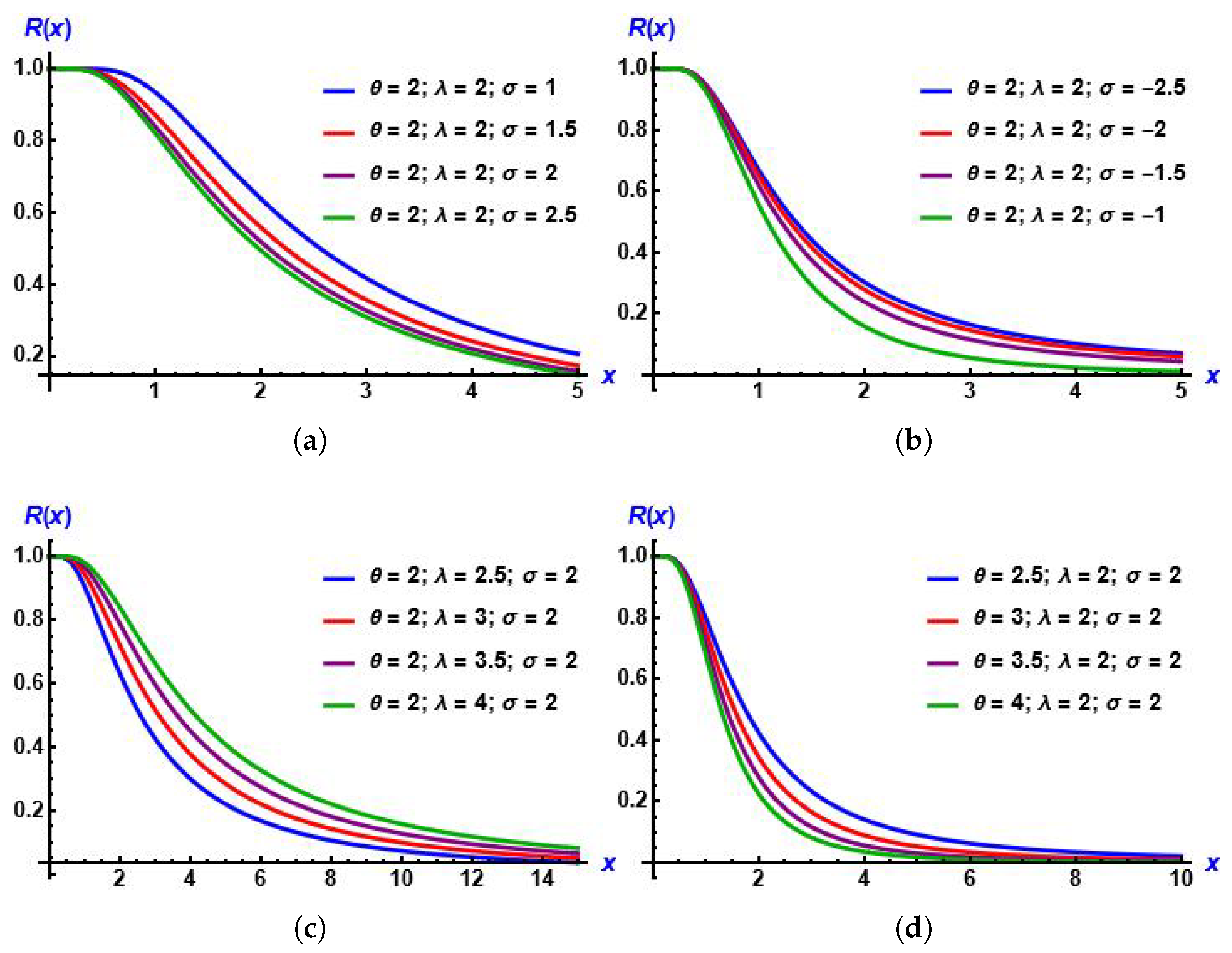
From plots in Figure 3, it is obvious that for any value of all parameters, the reliability function of the MGIE distribution decreases.

3.5. Hazard Function

The hazard function characterizes failure at a given time x, supposing that the object has survived up to that time. It is defined mathematically as
h ( x ) = g ( x ) 1 G ( x ) ,
Thus, the hazard function for the MGIE distribution can be obtained by substituting Equations (5) and (6) in Equation (27):
h ( x ) = θ λ x 2 e λ x ( 1 + 1 σ 2 σ ( 1 e λ x ) θ ) ( 1 e λ x ) ( 1 σ + 1 1 σ ( 1 e λ x ) θ ) .
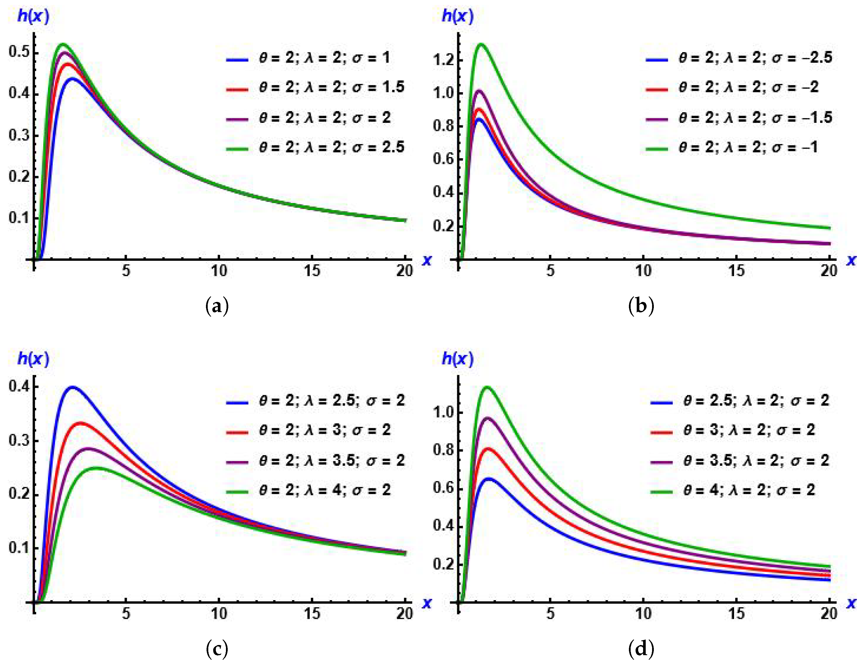
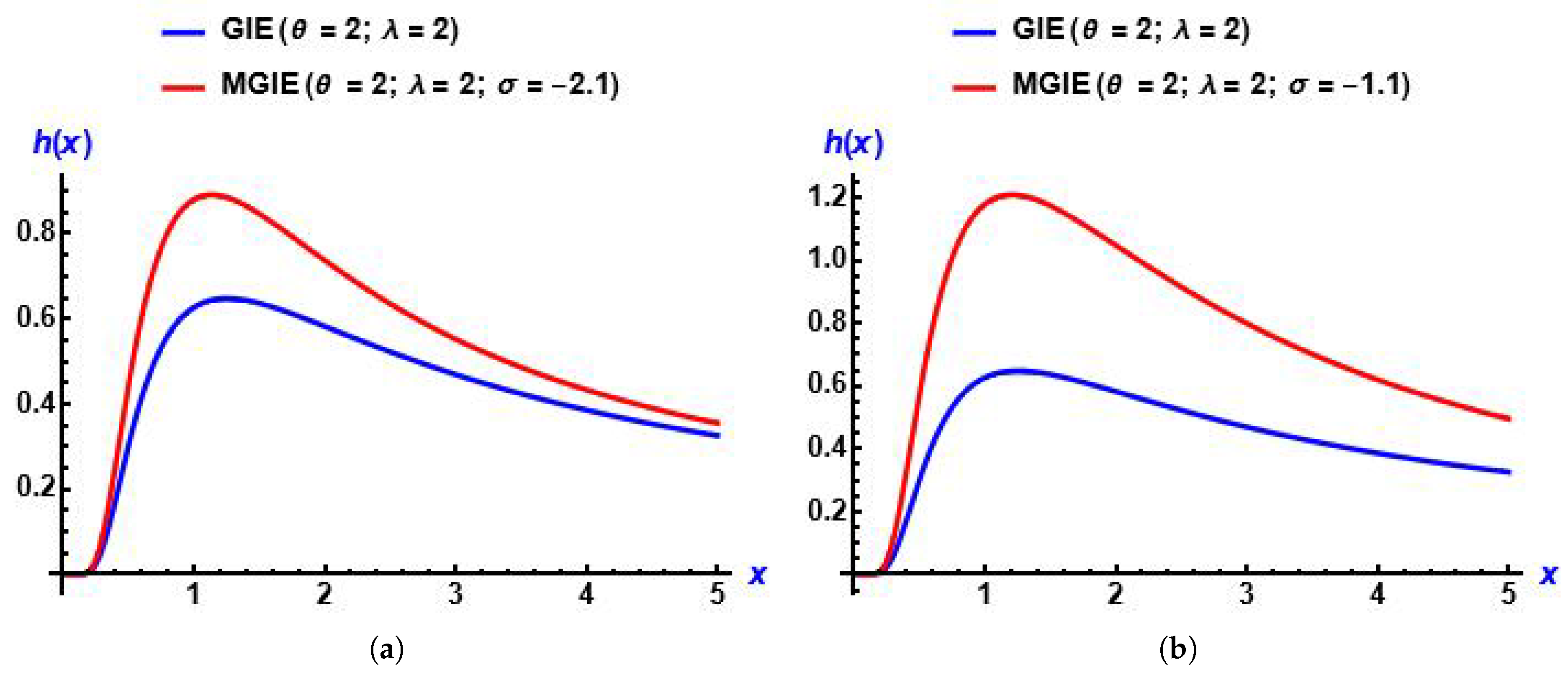
From plots in Figure 4, we can recognize that from several values of parameters, the curves of the hazard function are upside-down bathtub-shaped. Also, they increase then decrease, which is advantageous in survival analysis. In addition, Figure 5 shows the effect of the added parameter on the baseline distribution.

3.6. Mode

The mode can be found by deriving the PDF of the MGIE distribution with respect to x as follows:
d g ( x ) d x = 0 ,
By substituting Equation (5) in the previous equation, we obtain
f ( x ) [ 2 x + λ x 2 ( λ x 2 ( θ 1 ) e λ x ( 1 e λ x ) 1 ) + 2 θ λ σ x 2 e λ x ( 1 e λ x ) θ 1 ( 1 + 1 σ 2 σ ( 1 e λ x ) θ ) 1 ] = 0 ,
which gives
2 x + λ x 2 ( λ x 2 ( θ 1 ) e λ x ( 1 e λ x ) 1 ) + 2 θ λ σ x 2 e λ x ( 1 e λ x ) θ 1 ( 1 + 1 σ 2 σ ( 1 e λ x ) θ ) 1 = 0 .
As we can see, it is a non-linear equation. Therefore, we will use the Newton–Raphson method to solve this equation.

3.7. Odds Function

The odds function describes the ratio of an event to its non-occurrence. It is given by
O ( x ) = G ( x ) R ( x ) ,
by substituting Equations (6) and (25) with the previous equation:
O ( x ) = 1 [ ζ 1 e λ x i ζ 2 e λ x j ] τ ( ( 1 σ + 1 ) 1 σ τ ) ,
where ζ 1 , ζ 2 and τ are given in Equations (11), (12) and (26), respectively.
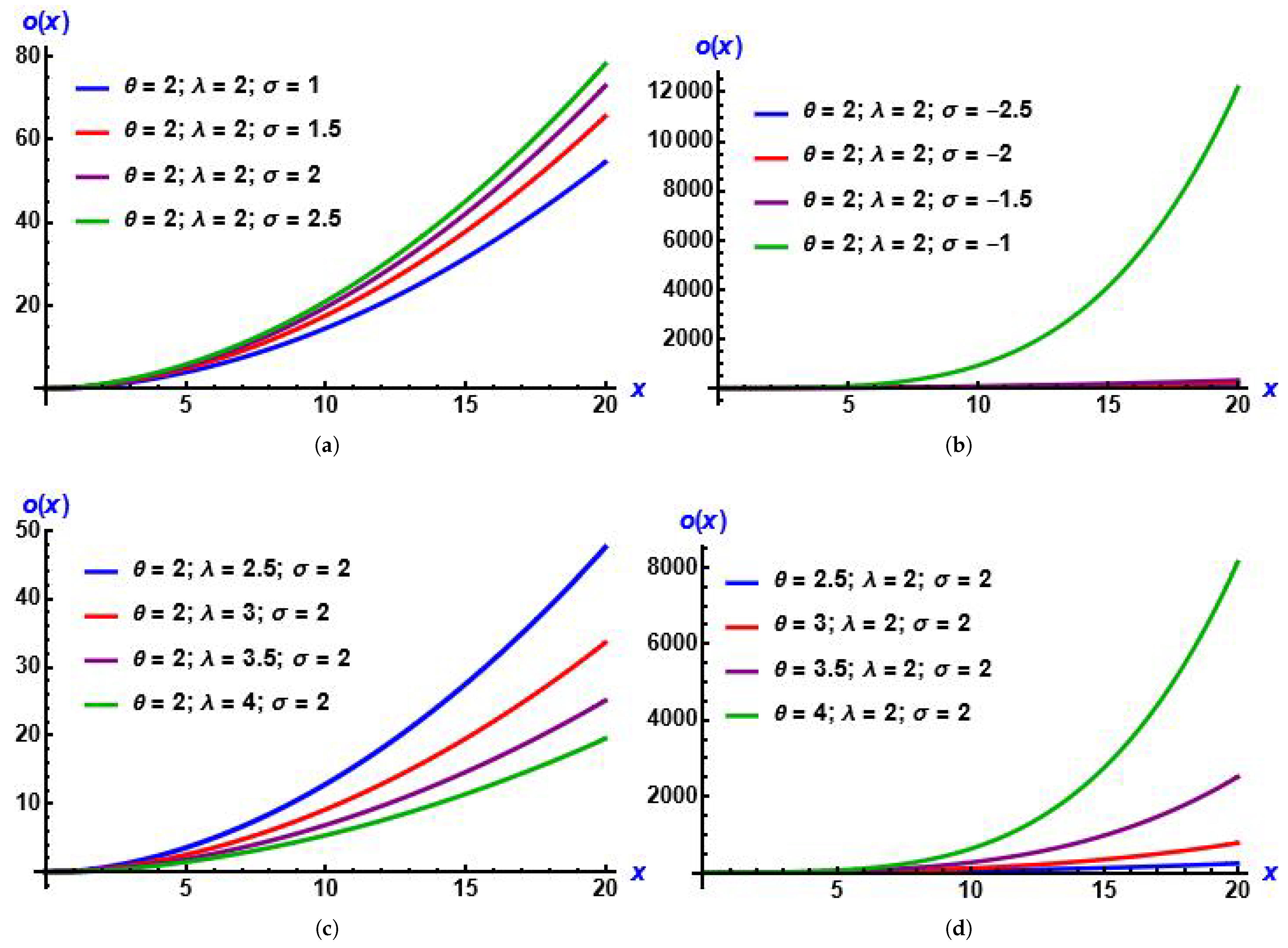
From Figure 6, we find that for various values of parameters, the odd function increases.

3.8. Harmonic Mean

If we have the adverse of a set of values x 1 , x 2 , , x n , the inverse of its arithmetic mean is known as the harmonic mean. It is defined by
H m ( x ) = 1 E ( 1 x ) = 1 0 x 1 g ( x ) d x ,
let
I = 0 x 1 g ( x ) d x ,
to derive the harmonic mean of the MGIE distribution, we use Equation (7) in the previous equation:
I = ψ 1 0 x 3 e λ x ( i + 1 ) d x + ψ 2 0 x 3 e λ x ( j + 1 ) d x ,
let
u = λ x ( i + 1 ) , w = λ x ( j + 1 ) ,
Thus, we get the harmonic mean of the MGIE distribution:
H m ( x ) = [ 1 λ 2 ( ψ 1 ( i + 1 ) 2 + ψ 2 ( j + 1 ) 2 ) ] 1 .
From Table 1, it is obvious that the alteration values of parameters of the MGIE distribution influence the behavior of its properties. Moreover, the MGIE distribution is unimodal and skewed to the right because, for any parameter values, the mode is less than the median and the median is less than mean. It is clear that if θ and σ increase, the mean, median, mode, harmonic mean, skewness, and kurtosis decrease. If λ increases, the mean, median, mode, and harmonic mean decrease, while the values of skewness and kurtosis do not change.

3.9. The Mean Deviation and the Median Deviation

The mean deviation and the median deviation are measures of dispersion that present data deviation from the mean and median. They can be found as follows:

3.9.1. The Mean Deviation About the Mean

We can derive the mean deviation about the mean as follows:
D ( μ ) = E x μ = 0 x μ g ( x ) d x .
To derive the mean deviation of the MGIE distribution, substitute Equation (10) in Equation (33); then, we get
D ( μ ) = 2 0 μ [ 1 ( ζ 1 e λ x i ζ 2 e λ x j ) ] d x = 2 [ μ ( ζ 1 ( μ 2 λ i e λ μ i ) ζ 2 ( μ 2 λ j e λ μ j ) ) ] ,
where ζ 1 and ζ 2 are given in Equations (11) and (12) respectively.

3.9.2. The Mean Deviation About the Median

We can derive the mean deviation about the median as follows:
D ( m ) = E x m = 0 x m g ( x ) d x ,
To derive the median deviation of the MGIE distribution, substitute Equation (10) in Equation (35); then, we get
D ( m ) = μ m + 2 0 m [ 1 ( ζ 1 e λ x i ζ 2 e λ x j ) ] d x = μ m + 2 [ m ( ζ 1 ( m 2 λ i e λ m i ) ζ 2 ( m 2 λ j e λ m j ) ) ] ,
where ζ 1 and ζ 2 are given in Equations (11) and (12), respectively.

3.10. Order Statistics

For a random sample x 1 , x 2 , , x n have the MGIE distribution with PDF g(x) and CDf G(x). The order statistics show that we should arrange these values in ascending order x 1 x 2 x n , and then the PDF of x j is defined as
g ( x j ) = n ! ( j 1 ) ! ( n j ) ! g ( x ) G ( x ) j 1 [ 1 G ( x ) ] n j ,
By substituting Equations (5) and (6) in the previous equation, we get the PDF of the order statistic x j :
g ( x j ) = n ! ( j 1 ) ! ( n j ) ! θ λ x j 2 e λ x j ( 1 e λ x j ) θ 1 [ 1 + 1 σ 2 σ ( 1 e λ x j ) θ ] × [ 1 ( 1 e λ x j ) θ ( 1 σ + 1 1 σ ( 1 e λ x j ) θ ) ] j 1 × [ 1 [ 1 ( 1 e λ x j ) θ ( 1 σ + 1 1 σ ( 1 e λ x j ) θ ) ] ] n j , x j > 0 .
We can find the PDF of the largest order statistic by using this formula:
g ( x n ) = n g ( x ) [ G ( x ) ] n 1 ,
thus
g ( x n ) = n θ λ x n 2 e λ x n ( 1 e λ x n ) θ 1 [ 1 + 1 σ 2 σ ( 1 e λ x n ) θ ] × [ 1 ( 1 e λ x n ) θ ( 1 σ + 1 1 σ ( 1 e λ x n ) θ ) ] n 1 , x n > 0 .
The smallest order statistic is given by using the following formula:
g ( x 1 ) = n g ( x ) [ 1 G ( x ) ] n 1 ,
thus
g ( x 1 ) = n θ λ x 1 2 e λ x 1 ( 1 e λ x 1 ) θ 1 [ 1 + 1 σ 2 σ ( 1 e λ x 1 ) θ ] × [ 1 [ 1 ( 1 e λ x 1 ) θ ( 1 σ + 1 1 σ ( 1 e λ x 1 ) θ ) ] ] n 1 , x 1 > 0 .

4. Rényi Entropy of the MGIE Distribution

Rényi entropy was introduced by [16]. It is considered to be one of the generalizations of Shannon’s entropy [17]. Entropy is used in many fields like physics and engineering. In physics, entropy is defined as the second law of thermodynamics. A thermodynamic system is considered to be a measure of the system’s disorder and that varies directly with any reversible change in heat in the system and inversely with the temperature of the system. In statistical mechanics, entropy is a measure of uncertainty, which remains relevant to a system after its macroscopic properties, such as temperature, pressure, and volume, have been observed.
Theorem 1.
The Rényi entropy of MGIE is given by
R δ ( x ) = 1 1 δ × l o g [ λ ( θ λ ) δ i = 0 n j = 0 n δ i ( θ 1 ) δ + θ i j ( 1 ) i + j ( 2 σ ) i ( 1 + 1 σ ) δ i ( Γ ( δ + 1 ) ( δ + j ) δ + 1 ) ] ,
The proof is given in Appendix A.1.

5. Parameters Estimation

5.1. Maximum Likelihood Estimation

This subsection extracts the maximum likelihood estimation, which is used to find estimators of parameters. Let x 1 , x 2 , , x n be a random sample from the MGIE distribution, then we can define the likelihood function by
L = i = 1 n g ( x i ) ,
The log-likelihood function is defined by
L = ( θ λ ) n i = 1 n ( x i ) 2 × e i = 1 n λ x i × i = 1 n ( 1 e λ x i ) θ 1 × i = 1 n ( 1 + 1 σ 2 σ ( 1 e λ x i ) θ ) ,
l = log L = n log ( θ ) + n log ( λ ) 2 i = 1 n log ( x i ) i = 1 n λ x i + ( θ 1 ) i = 1 n log ( 1 e λ x i ) + i = 1 n log ( 1 + 1 σ 2 σ ( 1 e λ x i ) θ ) ,
Differentiate the previous Equation (l) with respect to the parameters of our model θ , λ and σ , respectively.
All differentials are given in Appendix A.2.

5.2. Fisher Information

The Fisher method is used to obtain information for an unknown parameter by measuring another random, measurable variable.
Let ε ̲ = ( θ ^ , λ ^ , σ ^ ) is a community of parameters for the MGIE distribution. Then, the Fisher information matrix is given as
I ^ n 1 ( ε ^ ̲ ) = v a r ( θ ^ ) c o v ( θ ^ , λ ^ ) c o v ( θ ^ , σ ^ ) c o v ( λ ^ , θ ^ ) v a r ( λ ^ ) c o v ( λ ^ , σ ^ ) c o v ( σ ^ , θ ^ ) c o v ( σ ^ , λ ^ ) v a r ( σ ^ ) ,
I ^ n 1 ( ε ^ ̲ ) = ( ( 2 l o g l ε i ε j ) ) ε = ε ^ ,
To find this matrix, we need to find the second partial differentials of maximum likelihood estimation for all the parameters related to the distribution.
All differentials are given in Appendix A.3.

6. Simulation Study

To assess the efficiency of maximum likelihood estimators, in this section, we will find the estimates of the distribution parameters using the Mathematica (13.0) program and conduct simulations for different sample sizes, n = 10, 30, 50, 100, 150 and 200 from MGIE distribution. We will repeat the simulation N = 1000 and provide the maximum likelihood estimate (MLE), bias, mean squared error (MSE) and standard error (SE).
From Table 2 and Table 3, it is obvious that the maximum likelihood estimator is efficient and consistent, as we find that the MLE values approach the initial parameter with increasing sample size. In addition, we note that the bias, MSE, and SE become as low as possible.

7. Application

We will show the importance of the MGIE distribution by applying three real data points from bio-sciences fields. A method was used to estimate unknown parameters for the maximum likelihood estimation. To calculate this, we used Mathematica (13.0). We compared the suitability of the proposed distribution, which is the MGIE distribution with TIITLGIE distribution, exponentiated generalized inverted exponential distribution (EGIE) [18], Log-normal distribution [19], and Weibull distribution [20].
The comparison was performed according to the following criteria, so that the best distribution was the one with a lower value than the other distributions. The criteria were the Akaike information criterion (AIC) [21], Bayesian information criterion (BIC) [22], Corrected Akaike information criteria (CAIC) [23] and Hannan–Quinn information criterion (HQIC) [24].

7.1. Data Set 1

In this subsection, we show data from Saudi Arabia which consists of the number of deaths due to COVID-19 on 83 days, from 30 May to 20 August [25]: 17, 22, 23, 22, 24, 30, 32, 32, 34, 36, 34, 37, 36, 38, 36, 39, 40, 39, 41, 39, 48, 45, 46, 37, 40, 39, 41, 41, 46, 37, 40, 48, 50, 49, 54, 50, 56, 58, 52, 49, 42, 41, 51, 30, 42, 20, 40, 42, 45, 37, 40, 39, 37, 34, 44, 34, 37, 31, 30, 27, 29, 27, 26, 24, 21, 30, 32, 35, 36, 35, 38, 37, 37, 32, 34, 36, 34, 35, 31, 39, 28, 34, 36.
We will calculate the descriptive statistics for this data as shown in the Table 4.
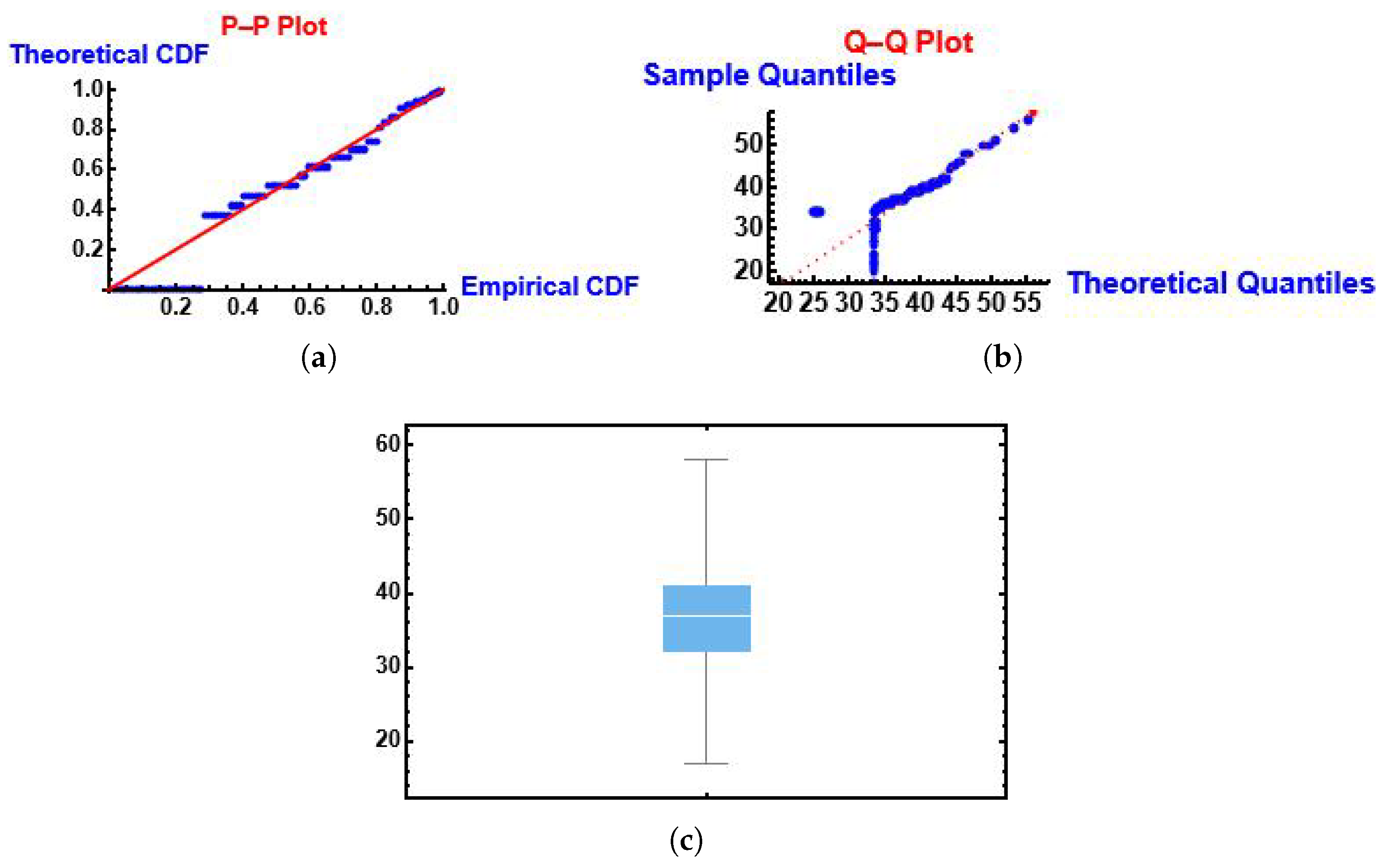
From Figure 7 we can see that the MGIE distribution follows the fitted PP (probability-probability) and QQ (quantile-quantile) functions. Also, we can see the box plot.
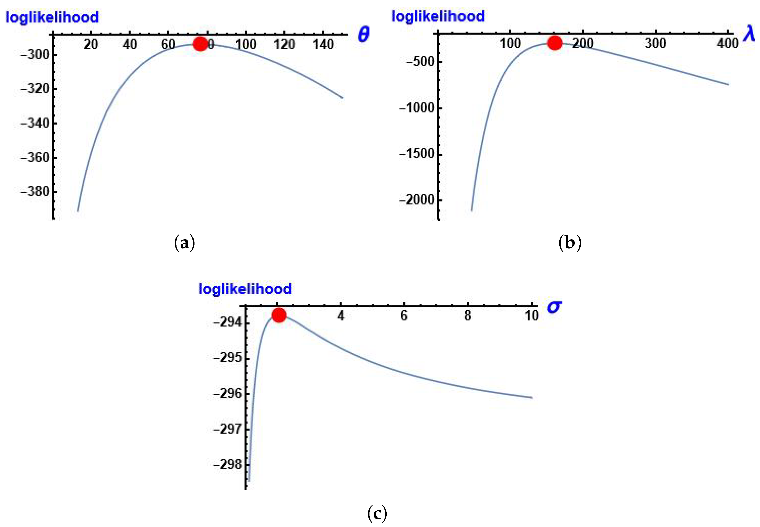
Figure 8 shows the log-likelihood function of the parameters of MGIE distribution θ , λ and σ using this data.
Table 5 presents the Kolmogorov-Smirnov test to determine the goodness of fit and the p-value for MGIE distribution and competing models.
From Table 6 we note that the MGIE distribution consistently outperforms competitive distributions in all the criteria used for the study. This gives the MGIE distribution practically significant and supports its use as a flexible and effective alternative.
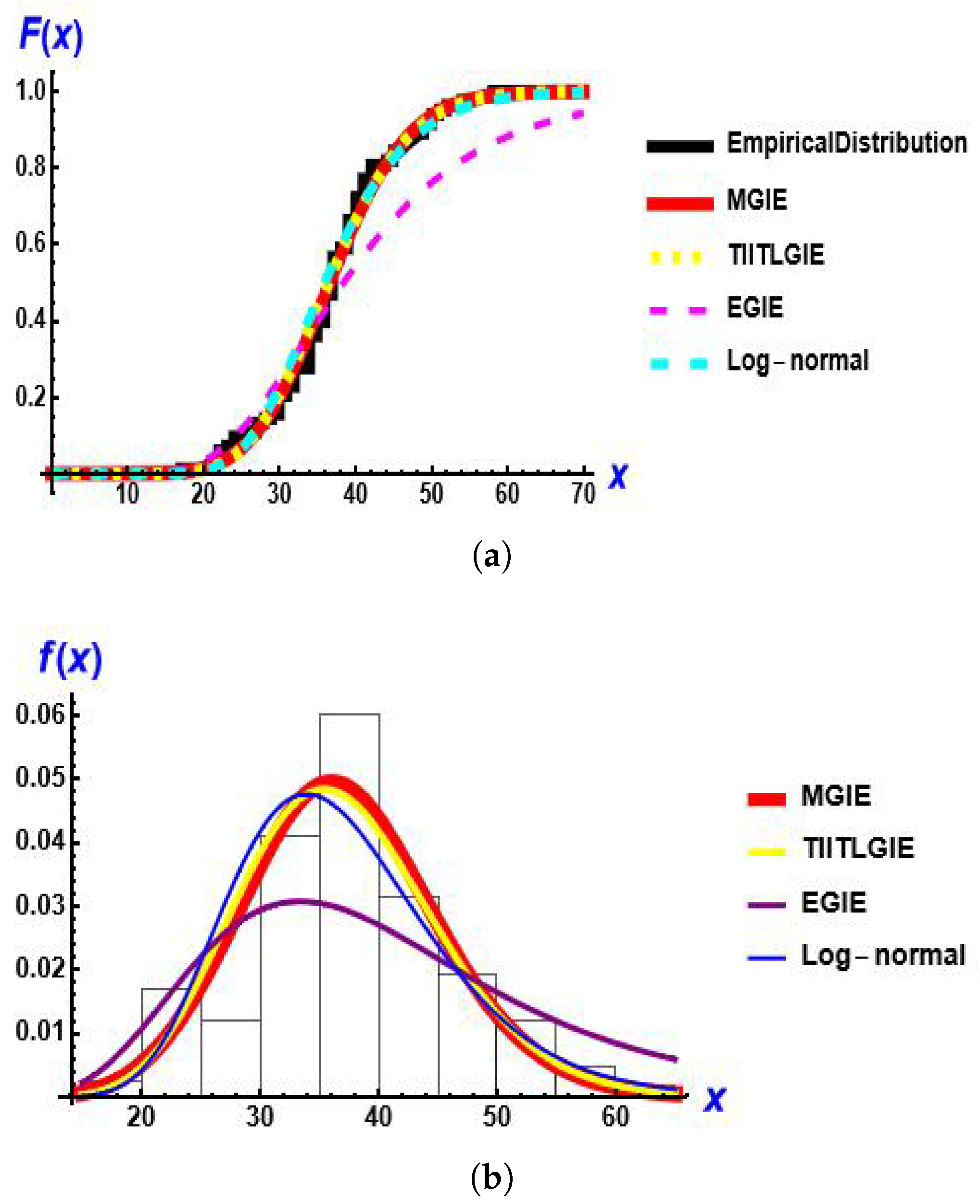
Figure 9 presents the empirical distribution, estimated CDF and estimated PDF for the models for this data set.

7.2. Data Set 2

This data shows the rainfall recorded in Los Angeles (30 June–1 July) in the period (1962–2012) [10]: 3.21, 4.42, 7.17, 7.22, 7.35, 7.66, 7.77, 7.93, 8.08, 8.11, 8.38, 8.69, 8.98, 9.08, 9.09, 9.24, 10.43, 10.71, 11.47, 11.57, 12.31, 12.32, 12.4, 12.46, 12.48, 12.82, 13.19, 13.53, 13.69, 14.35, 14.92, 16.36, 16.49, 16.58, 17.86, 17.94, 19.67, 20.2, 20.44, 21.0, 21.26, 22.0, 24.35, 26.98, 27.36, 27.47, 31.01, 31.25, 33.44, 37.25
We will calculate the descriptive statistics for this data as shown in the Table 7.
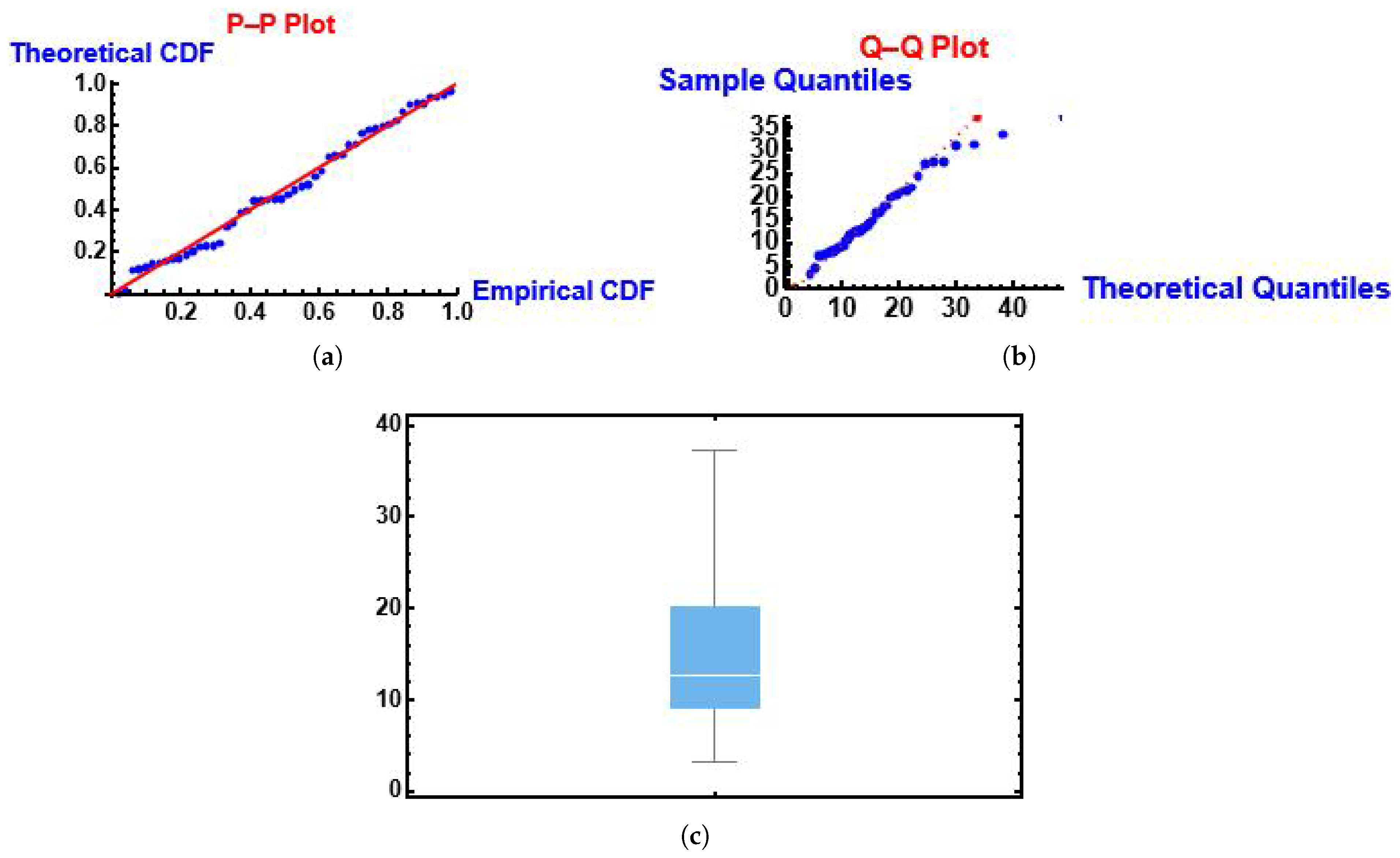
From Figure 10 we can see that the MGIE distribution follows the fitted PP (probability-probability) and QQ (quantile-quantile) functions. Also, we can see the box plot.
Table 8 presents the Kolmogorov-Smirnov test to determine the goodness of fit and the p-value for MGIE distribution and competing models.
From Table 9 we note that the MGIE distribution consistently outperforms competitive distributions in all the criteria used for the study. This gives the MGIE distribution practically significant and supports its use as a flexible and effective alternative.
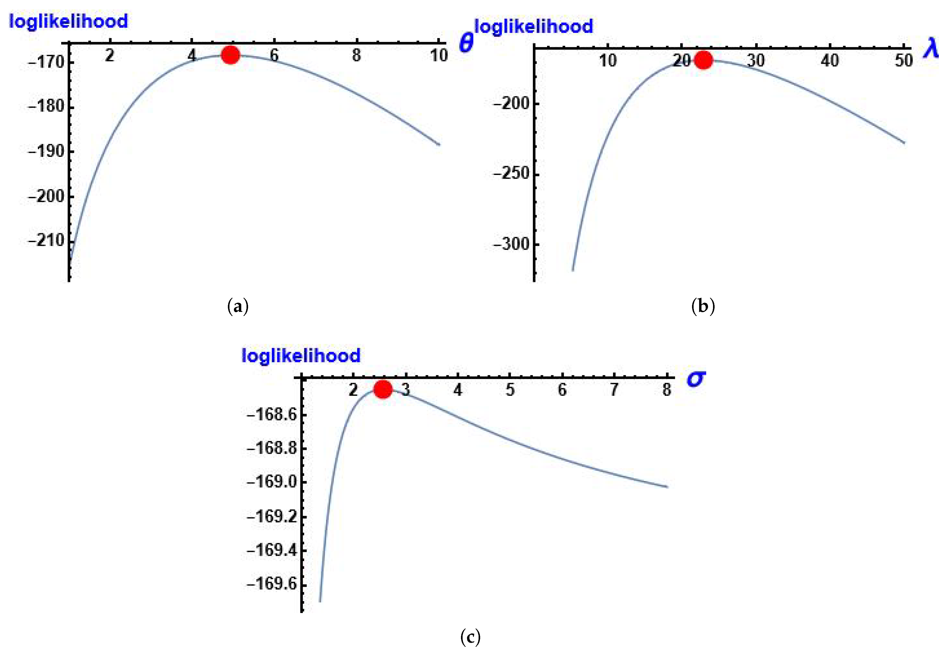
Figure 11 shows the log-likelihood function of the parameters of MGIE distribution θ , λ and σ using this data.
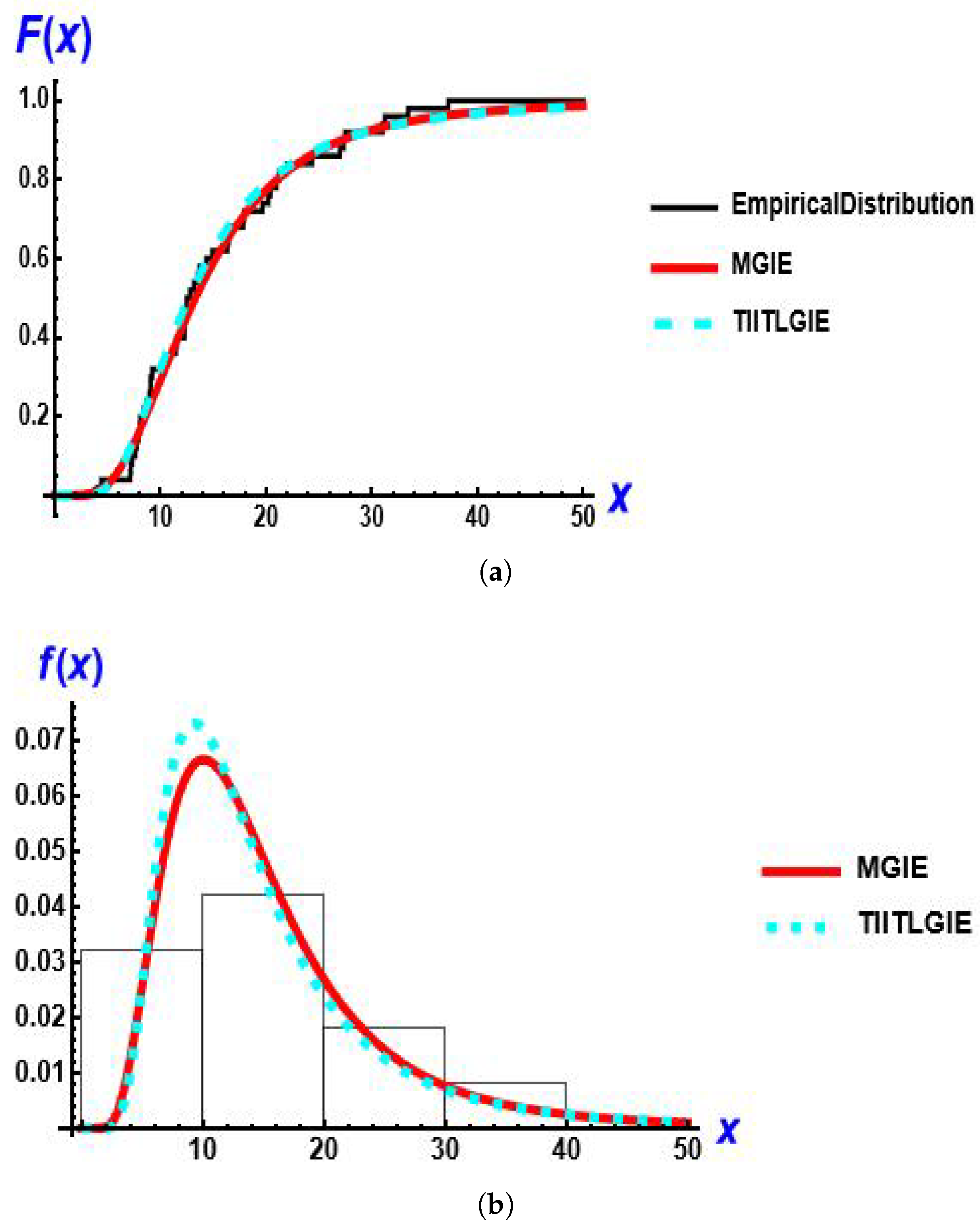
Figure 12 presents the empirical distribution, estimated CDF and estimated PDF for the models for this data set.

7.3. Data Set 3

This data shows the lifespans of patients undergoing analgesic treatment [26]: 1.4, 1.1, 1.7, 1.3, 1.8, 1.9, 2.2, 1.6, 2.7, 1.7, 1.8, 4.1, 1.2, 1.5, 3, 1.4, 2.3, 1.7, 2.0, 1.6.
We will calculate the descriptive statistics for this data as shown in the Table 10.
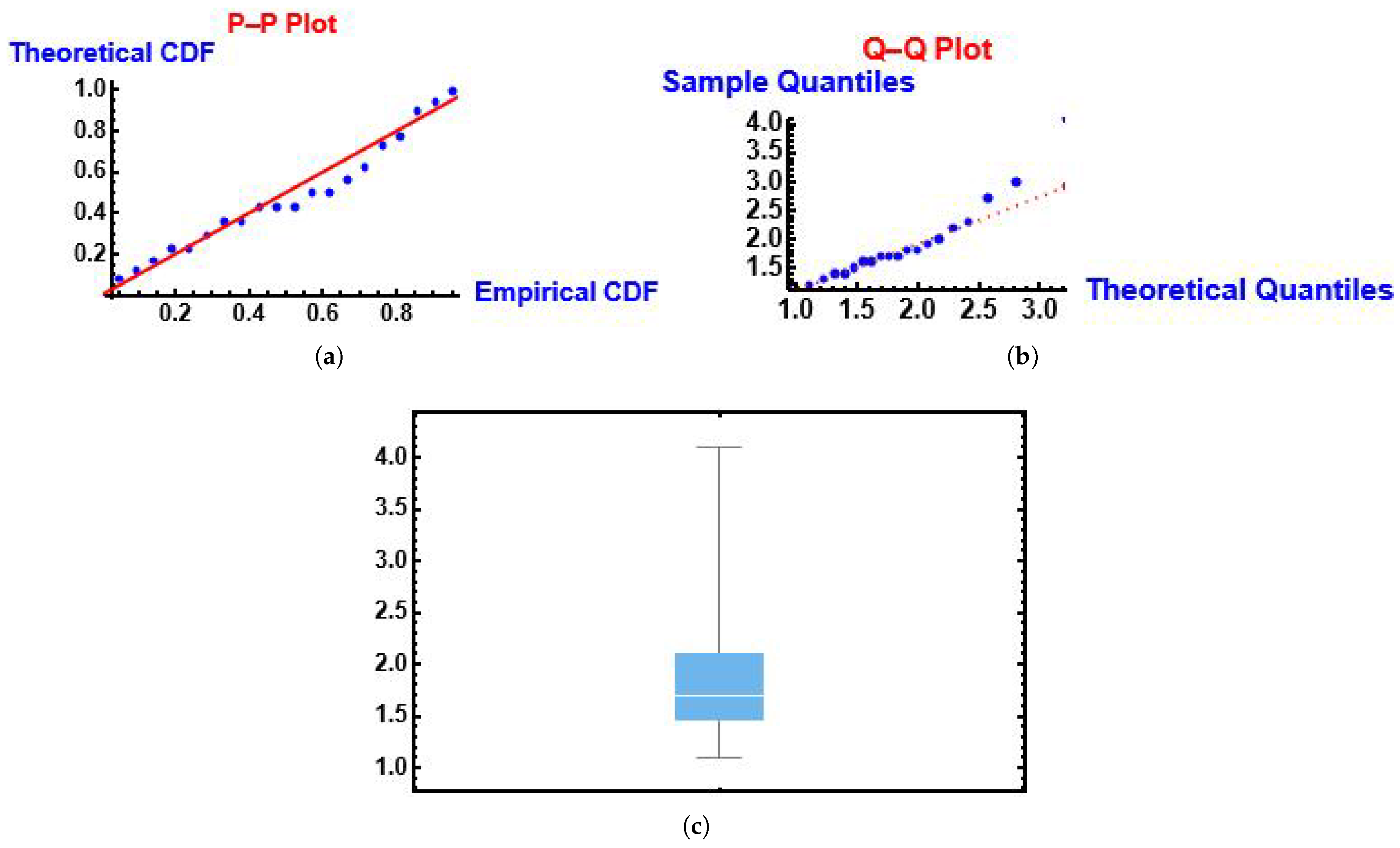
From Figure 13 we can see that the MGIE distribution follows the fitted PP (probability-probability) and QQ (quantile-quantile) functions. Also, we can see the box plot.
Table 11 presents the Kolmogorov-Smirnov test to determine the goodness of fit and the p-value for MGIE distribution and competing models.
From Table 12 we note that the MGIE distribution consistently outperforms competitive distributions in all the criteria used for the study. This gives the MGIE distribution practically significant and supports its use as a flexible and effective alternative.
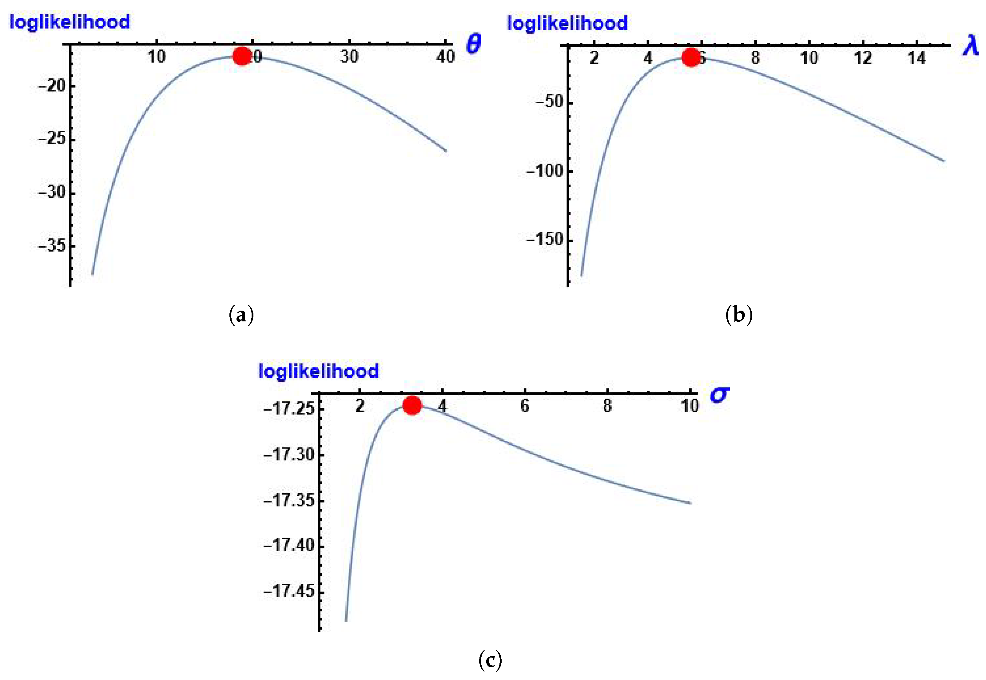
Figure 14 shows the log-likelihood function of the parameters of MGIE distribution θ , λ and σ using this data.
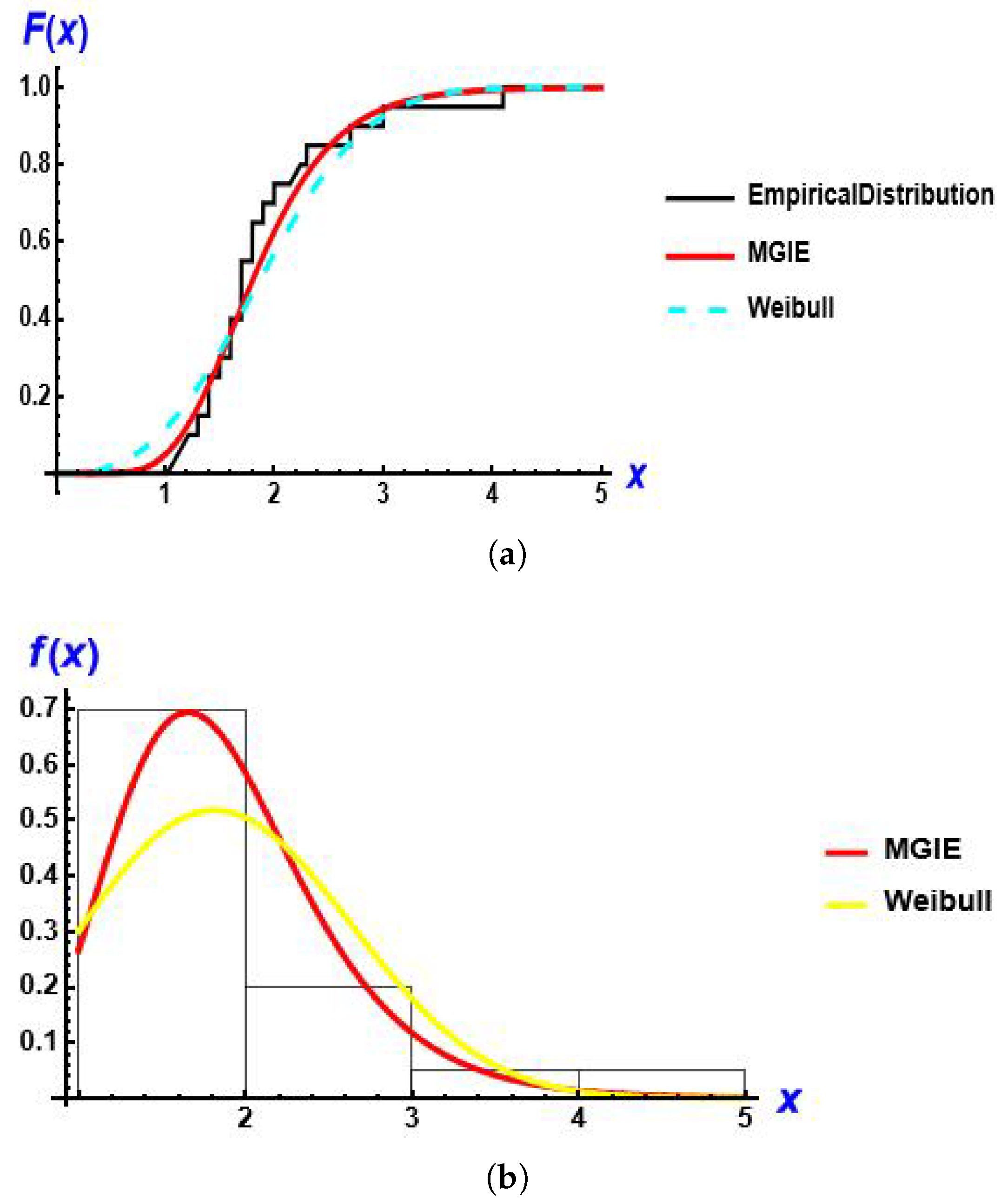
Figure 15 presents the empirical distribution, estimated CDF and estimated PDF for the models for this data set.

8. Conclusions

In this research, we presented a three-parameter Modified Generalized Inverted Exponential Distribution. Also, some important statistical properties are studied. The unknown parameters are estimated. In addition, we performed a simulation study to study the behavior of the estimators and present an application using real data from bio-sciences fields. As is clearly evident, our suggested distribution is more suitable than other related distributions.
Also, we present several propositions that can be helpful in future work, such as using the Bayesian methods to estimate the parameters of MGIED, estimating the three parameters of MGIED under several kinds of censored samples, and applying the model to different data areas in the field of bio-sciences data and in other fields.

Author Contributions

Methodology, Z.A.A.-S.; Software, H.H.A.-J.; Validation, Z.A.A.-S.; Resources, H.H.A.-J.; Writing—original draft, H.H.A.-J.; Writing—review & editing, H.H.A.-J.; Visualization, H.H.A.-J.; Supervision, Z.A.A.-S. All authors have read and agreed to the published version of the manuscript.

Funding

This work was funded by the University of Jeddah, Jeddah, Saudi Arabia, under grant No. (UJ-22-DR-36). The authors, therefore, acknowledge with thanks the University of Jeddah for its technical and financial support.

Institutional Review Board Statement

Not applicable.

Data Availability Statement

The original contributions presented in this study are included in the article. Further inquiries can be directed to the corresponding authors.

Conflicts of Interest

The authors declare no conflict of interest.

Abbreviations

The following abbreviations are used in this manuscript:
NModi-GNew modified-G (NModi-G) family
CDFCumulative Distribution Function
PDFProbability Density Function
GIEDGeneralized Inverted Exponential Distribution
TLGIETopp–Leone Inverted Exponential Distribution
TIITLGIEType II Topp-Leone Generalized Inverted Exponential Distribution
MGIEModified Generalized Inverted Exponential
G ( y ; σ , ϕ ) CDF of NModi-G family
g ( y ; σ , ϕ ) PDF of NModi-G family
F ( x ) CDF of GIED
f ( x ) PDF of GIED
G ( x ) CDF of MGIE
g ( x ) PDF of MGIE
MIEModified Inverse Exponential
MSIEModified Standard Inverse Exponential
MGSIEModified Generalized Standard Inverse Exponential
Q(u)Quantile Function
mMedian
μ r ´ The r t h Moment
E r ( 1 ) Generalized Exponential Integral Function
M x ( t ) Moment-Generating Function (MGF)
BBowley’s Coefficient of Skewness
MMoors’ Coefficient of Kurtosis
R(x)Reliability Function
h(x)Hazard Function
O(x)Odds Function
H m ( x )        Harmonic Mean
D ( μ ) Mean Deviation
D ( m ) Median Deviation
g ( x j ) Order Statistics
g ( x n ) Largest Order Statistic
g ( x 1 ) Smallest Order Statistic
R δ ( x ) Rényi entropy
LLikelihood Function
lLog-Likelihood Function
IEInverted Exponential Distribution
EExponential Distribution
EGIEExponentiated generalized inverted exponential distribution
AICAkaike Information Criterion
BICBayesian Information Criterion
CAICCorrected Akaike Information Criteria
HQICHannan–Quinn information criterion
MLElikelihood estimate
MSEMean squared error
SEStandard Error
SDStandard deviation

Appendix A

Appendix A.1

Proof of Theorem 1.
Suppose the g ( x ) is the pdf of the MGIE distribution, then the Rényi entropy is derived as follow:
R δ ( x ) = 1 1 δ ( l o g [ J ( δ ) ] ) ,
such that the:
J ( δ ) = 0 g δ ( x ) d x ; δ > 0 and δ 1 ,
by using Equation (5) in the previous equation:
J ( δ ) = 0 ( θ λ x 2 ) δ e λ x δ ( 1 e λ x ) ( θ 1 ) δ ( 1 + 1 σ 2 σ ( 1 e λ x ) θ ) δ d x ,
suppose
u = λ x ,
therefore
J ( δ ) = 0 λ ( θ u 2 λ ) δ e u δ ( 1 e u ) ( θ 1 ) δ [ 1 + 1 σ 2 σ ( 1 e u ) θ ] δ 1 u 2 d u ,
we derived the following equation by using binomial expansion
J ( δ ) = 0 λ ( θ u 2 λ ) δ e u δ ( 1 e u ) ( θ 1 ) δ × [ i = 0 n δ i ( 1 ) i ( 2 σ ( 1 e u ) θ ) i ( 1 + 1 σ ) δ i ] 1 u 2 d u ,
J ( δ ) = λ ( θ λ ) δ i = 0 n δ i ( 1 ) i ( 2 σ ) i ( 1 + 1 σ ) δ i 0 e u δ ( 1 e u ) ( θ 1 ) δ + θ i u δ d u ,
we derive the Rényi entropy for MGIE distribution as follow:
R δ ( x ) = 1 1 δ × l o g [ λ ( θ λ ) δ i = 0 n j = 0 n δ i ( θ 1 ) δ + θ i j ( 1 ) i + j ( 2 σ ) i ( 1 + 1 σ ) δ i ( Γ ( δ + 1 ) ( δ + j ) δ + 1 ) ] ,

Appendix A.2

l θ = n θ + i = 1 n log ( 1 e λ x i ) 2 σ i = 1 n ( 1 e λ x i ) θ log ( 1 e λ x i ) 1 + 1 σ 2 σ ( 1 e λ x i ) θ = 0 ,
l λ = n λ i = 1 n 1 x i + ( θ 1 ) i = 1 n e λ x i x i ( 1 e λ x i ) 2 θ σ i = 1 n e λ x i ( 1 e λ x i ) θ 1 x i ( 1 + 1 σ 2 σ ( 1 e λ x i ) θ ) = 0 ,
l σ = i = 1 n 1 σ 2 + 2 σ 2 ( 1 e λ x i ) θ 1 + 1 σ 2 σ ( 1 e λ x i ) θ = 0 .
Mathematica (13.0) will be used to find the maximum likelihood estimates of our parameters θ ^ , λ ^ and σ ^ numerically.

Appendix A.3

2 l o g l θ 2 = n θ 2 2 σ i = 1 n [ ( 1 e λ x i ) θ l o g ( 1 e λ x i ) 2 1 + 1 σ 2 σ ( 1 e λ x i ) θ 2 σ ( 1 e λ x i ) 2 θ l o g ( 1 e λ x i ) 2 ( 1 + 1 σ 2 σ ( 1 e λ x i ) θ ) 2 ] ,
2 l o g l λ 2 = n λ 2 + ( θ 1 ) i = 1 n [ e λ x i x i 2 ( 1 e λ x i ) e 2 λ x i x i 2 ( 1 e λ x i ) 2 ] 2 θ σ i = 1 n [ e λ x i ( ( θ 1 ) e λ x i ( 1 e λ x i ) θ 2 ( 1 e λ x i ) θ 1 ) x i 2 ( 1 + 1 σ 2 σ ( 1 e λ x i ) θ ) 2 θ σ e 2 λ x i ( 1 e λ x i ) 2 θ 2 x i 2 ( 1 + 1 σ 2 σ ( 1 e λ x i ) θ ) 2 ] ,
2 l o g l σ 2 = i = 1 n [ 2 σ 3 4 σ 3 ( 1 e λ x i ) θ 1 + 1 σ 2 σ ( 1 e λ x i ) θ ( 1 σ 2 + 2 σ 2 ( 1 e λ x i ) θ ) 2 ( 1 + 1 σ 2 σ ( 1 e λ x i ) θ ) 2 ] ,
2 l o g l θ λ = i = 1 n [ e λ x i x i ( 1 e λ x i ) ] 2 σ i = 1 n [ ( 1 e λ x i ) θ 1 e λ x i ( θ l o g ( 1 e λ x i ) + 1 ) x i ( 1 + 1 σ 2 σ ( 1 e λ x i ) θ ) 2 θ σ e λ x i ( 1 e λ x i ) 2 θ 1 l o g ( 1 e λ x i ) x i ( 1 + 1 σ 2 σ ( 1 e λ x i ) θ ) 2 ] ,
2 l o g l σ θ = i = 1 n [ 2 σ 2 ( 1 e λ x i ) θ l o g ( 1 e λ x i ) ( 1 + 1 σ 2 σ ( 1 e λ x i ) θ ) ( 1 σ 2 + 2 σ 2 ( 1 e λ x i ) θ ) ( 2 σ ( 1 e λ x i ) θ l o g ( 1 e λ x i ) ) ( 1 + 1 σ 2 σ ( 1 e λ x i ) θ ) 2 ] ,
2 l o g l σ λ = i = 1 n [ 2 θ σ 2 ( 1 e λ x i ) θ 1 e λ x i x i ( 1 + 1 σ 2 σ ( 1 e λ x i ) θ ) ( 1 σ 2 + 2 σ 2 ( 1 e λ x i ) ) ( 2 θ σ ( 1 e λ x i ) θ 1 e λ x i ) x i ( 1 + 1 σ 2 σ ( 1 e λ x i ) θ ) 2 ] .

References

  1. Cordeiro, G.M.; Ortega, E.M.; da Cunha, D.C.C. The exponentiated generalized class of distributions. J. Data Sci. 2022, 11, 1–27. [Google Scholar] [CrossRef]
  2. Bantan, R.A.R.; Jamal, F.; Chesneau, C.; Elgarhy, M. Type II power Topp-Leone generated family of distribution with statistical inference and applications. Symmetry 2020, 12, 75. [Google Scholar] [CrossRef]
  3. Cordeiro, G.M.; Ortega, E.M.; Popovi, B.V.; Pescim, R.R. The Lomax generator of distributions: Properties, minification process and regression model. Appl. Math. Comput. 2014, 247, 465–486. [Google Scholar] [CrossRef]
  4. Arif, M.; Khan, D.M.; Khosa, S.K.; Aamir, M.; Aslam, A.; Ahmad, Z. Modelling insurance losses with a new family of heavy-tailed distributions. Comput. Mater. Contin. 2020, 66, 537–550. [Google Scholar] [CrossRef]
  5. Alshawarbeh, E. A New Modified-X family of distributions with applications in modeling biomedical data. Alex. Eng. J. 2024, 93, 189–206. [Google Scholar] [CrossRef]
  6. Al-Shomrani, A.A.; Shawky, A.I. A New Family of Distributions: Properties and Applications. Adv. Appl. Stat. 2024, 91, 257–300. [Google Scholar] [CrossRef]
  7. El-Morshedy, M.; Ahmad, Z.; tag-Eldin, E.; Almaspoor, Z.; Eliwa, M.S.; Iqbal, Z. A new statistical approach for modeling the bladder cancer and leukemia patients data sets: Case studies in the medical sector. Math. Biosci. Eng. 2022, 19, 10474–10492. [Google Scholar] [CrossRef]
  8. Abouammoh, A.M.; Alshingiti, A.M. Reliability estimation of generalized inverted exponential distribution. J. Stat. Comput. Simul. 2009, 79, 1301–1315. [Google Scholar] [CrossRef]
  9. Al-Saiary, Z.A.; Bakoban, R.A. The Topp-Leone generalized inverted exponential distribution with real data applications. Entropy 2020, 22, 1144. [Google Scholar] [CrossRef] [PubMed]
  10. Al-Saiary, Z.A.; Al-Jadaani, S.H. Type II Topp Leone generalized inverted exponential distribution with real data applications. Asian J. Probab. Stat. 2022, 16, 37–51. [Google Scholar] [CrossRef]
  11. Zhang, H.; Wu, J.; Gui, W. Inferences on the Generalized Inverted Exponential Distribution in Constant Stress Partially Accelerated Life Tests Using Generally Progressively Type-II Censored Samples. Appl. Sci. 2024, 14, 6050. [Google Scholar] [CrossRef]
  12. Sarhan, A.M.; Gomaa, R.S.; Magar, A.A.; Alsadat, N. Bivariate exponentiated generalized inverted exponential distribution with applications on dependent competing risks data. AIMS Math. 2024, 9, 29439–29473. [Google Scholar] [CrossRef]
  13. Abo-Kasem, O.E.; Abu-El AzmWael, W.S.; Sherif, B.K. Estimation of Generalized Inverted Exponential Distribution under Generalized Hybrid Censoring Scheme. J. Bus. Res. 2025, 47, 224–261. [Google Scholar]
  14. Kenney, J.F.; Keeping, E.S. Mathematics of Statistics, 3rd ed.; Van Nostrand: New York, NJ, USA, 1962; p. 101. [Google Scholar]
  15. Keller, A.Z.; Kamath, A.R.R.; Perera, U.D. Reliability analysis of CNC machine tools. Reliab. Eng. 1982, 3, 449–473. [Google Scholar] [CrossRef]
  16. Rényi, A. On the dimension and entropy of probability distributions. Acta Math. Acad. Sci. Hung. 1959, 10, 193–215. [Google Scholar] [CrossRef]
  17. Shannon, C.E. A Mathematical theory of communication. Bell Syst. Tech. J. 1948, 27, 379–423. [Google Scholar] [CrossRef]
  18. Oguntunde, P.E.; Adejumo, A.; Balogun, O.S. Statistical Properties of the Exponentiated Generalized Inverted Exponential Distribution. Appl. Math. 2014, 4, 47–55. [Google Scholar]
  19. Moral de la Rubia, J. Lognormal distribution for social researchers: A probability classic. Int. J. Psychol. Couns. 2024, 16, 10–25. [Google Scholar]
  20. Weibull, W. A statistical distribution function of wide applicability. J. Appl. Mech. 1951, 18, 293–297. [Google Scholar] [CrossRef]
  21. Akaike, H. A New Look at the Statistical Model Identification. IEEE Trans. Autom. Control 1974, 19, 716–723. [Google Scholar] [CrossRef]
  22. Schwarz, G. Estimating the Dimension of a Model. Ann. Stat. 1978, 6, 461–464. [Google Scholar] [CrossRef]
  23. Hurvich, C.M.; Tsai, C.L. A corrected Akaike information criterion for vector autoregressive model selection. J. Time Ser. Anal. 1993, 14, 271–279. [Google Scholar] [CrossRef]
  24. Hannan, E.J.; Quinn, B.G. The determination of the order of an autoregression. J. R. Stat. Soc. Ser. B 1979, 41, 190–195. [Google Scholar] [CrossRef]
  25. Al-Saiary, Z. A new extended “A” distribution with real data applications. Adv. Appl. Stat. 2023, 90, 257–287. [Google Scholar] [CrossRef]
  26. Shah, Z.; Abdalla, G.S.S.; Khan, D.M.; Rao, G.S.; Jamal, F.; Almetwally, E.M. A logarithmic exponent power half Logistic-G family of distributions: Repetitive acceptance sampling plan and applications to engineering and radiation sectors. J. Radiat. Res. Appl. Sci. 2025, 18, 101797. [Google Scholar] [CrossRef]
Figure 1. Plots of the PDF of the MGIE distribution for diverse values of the parameters. (a) σ increases; (b) σ decreases; (c) λ increases; (d) θ increases.
Entropy 28 00161 g001
Figure 2. Plots of the PDF of the GIED and MGIE distributions for diverse values of the parameters. (a) σ is positive; (b) σ is negative.
Entropy 28 00161 g002
Figure 3. Plots of reliability function of the MGIE distribution for diverse values of the parameters. (a) σ increases; (b) σ decreases; (c) λ increases; (d) θ increases.
Entropy 28 00161 g003
Figure 4. Plots of hazard function of the MGIE distribution for diverse values of the parameters. (a) σ increases; (b) σ decreases; (c) λ increases; (d) θ increases.
Entropy 28 00161 g004
Figure 5. Plots of hazard function of the GIED and MGIE distributions for diverse parameter values. (a) σ is negative; (b) σ is negative.
Entropy 28 00161 g005
Figure 6. Plots of odds function of the MGIE distribution for diverse values of the parameters. (a) σ increases; (b) σ decreases; (c) λ increases; (d) θ increases.
Entropy 28 00161 g006
Figure 7. PP, QQ and box plots of the MGIE distribution using the number of deaths due to COVID-19 data. (a) PP plot; (b) QQ plot; (c) box plot.
Entropy 28 00161 g007
Figure 8. The profile of the log-likelihood function of the parameters using data about the number of deaths due to COVID-19. (a) log-likelihood function of θ ; (b) log-likelihood function of λ ; (c) log-likelihood function of σ .
Entropy 28 00161 g008
Figure 9. The fitted CDF and PDF Plots of the MGIE distribution compared to other distributions using data on the number of deaths due to COVID-19. (a) estimated CDF; (b) estimated PDF.
Entropy 28 00161 g009
Figure 10. PP, QQ and box plots of the MGIE distribution using rainfall data. (a) PP plot; (b) QQ plot; (c) box plot.
Entropy 28 00161 g010
Figure 11. The profile of the log-likelihood function of the parameters using rainfall data. (a) log-likelihood function of θ ; (b) log-likelihood function of λ ; (c) log-likelihood function of σ .
Entropy 28 00161 g011
Figure 12. The fitted CDF and PDF plots of the MGIE distribution compared to other distributions using rainfall data. (a) estimated CDF; (b) estimated PDF.
Entropy 28 00161 g012
Figure 13. PP, QQ and box plots of the MGIE distribution using data of lifespans of patients undergoing analgesic treatment. (a) PP plot; (b) QQ plot; (c) box plot.
Entropy 28 00161 g013
Figure 14. The profile of the log-likelihood function of the parameters using data on the lifespans of patients undergoing analgesic treatment. (a) log-likelihood function of θ ; (b) log-likelihood function of λ ; (c) log-likelihood function of σ .
Entropy 28 00161 g014
Figure 15. The fitted CDF and PDF plots of the MGIE distribution compared to other distributions using data of lifespans of patients undergoing analgesic treatment. (a) estimated CDF; (b) estimated PDF.
Entropy 28 00161 g015
Table 1. The mean, median, mode, harmonic mean, skewness, and kurtosis of the MGIE distribution.
θ λ σ MeanMedianModeHarmonic MeanSkewnessKurtosis
2214.185992.566961.493852.181820.3200471.58616
221.53.714852.24051.267991.80.3159471.58364
2223.479292.078091.141251.655170.3172131.58293
222.53.337951.982351.06981.578950.3191891.58359
22−2.52.207231.352010.8099421.153850.316161.59818
22−22.065891.296610.7989971.116280.3061281.58218
22−1.51.830321.215430.7843721.058820.284251.53551
22−11.359191.088020.7639370.960.2301641.39708
22.524.349112.597611.426562.068970.3172131.58293
2325.218933.117131.711872.482760.3172131.58293
23.526.088753.636651.997182.896550.3172131.58293
2426.958574.156172.282493.310340.3172131.58293
2.5222.537521.752991.079381.450440.2787661.49894
3222.066381.546751.028241.311480.2509951.44738
3.5221.781531.403110.9854621.210140.2297591.41264
4221.589451.296610.9491551.132460.212851.3877
Table 2. The MLE Estimates, bias, MSE and SE of MGIE for the unknown parameters θ ^ , λ ^ and σ ^ with the initial values ( θ = 0.2, λ = 0.7, σ = 1.5).
θ = 0.2, λ = 0.7, σ = 1.5
nParameters MLE Bias MSE SE
10 θ ^ 0.2369090.03690950.008075380.00259226
λ ^ 1.594470.8944748.814760.0895695
σ ^ 1.514590.01459330.4433110.0210604
30 θ ^ 0.2107930.01079260.001324440.00109962
λ ^ 0.8173890.1173890.3311740.0178245
σ ^ 1.572230.07222690.4986650.0222248
50 θ ^ 0.2076480.007648130.0007903270.000855901
λ ^ 0.7975760.09757590.2101050.0141699
σ ^ 1.597250.09724870.4658880.0213749
75 θ ^ 0.199697−0.000303430.0007785370.000882737
λ ^ 0.7537870.05378740.1384750.0116498
σ ^ 1.661740.1617380.4702340.0210836
100 θ ^ 0.2015080.001508260.0003976910.000629136
λ ^ 0.688347−0.01165310.09744990.00986973
σ ^ 1.552080.05208380.397110.0198694
150 θ ^ 0.2024350.002434590.0002607340.000505036
λ ^ 0.659425−0.04057530.0785730.00877517
σ ^ 1.602640.1026440.5104320.0223696
200 θ ^ 0.198672−0.001328070.0002088360.000455279
λ ^ 0.7099070.00990710.04954770.00703555
σ ^ 1.730480.2304780.4124190.0189647
Table 3. The MLE Estimates, bias, MSE and SE of MGIE for the unknown parameters θ ^ , λ ^ and σ ^ with the initial values ( θ = 2, λ = 2, σ = 3).
θ = 2, λ = 2, σ = 3
n Parameters MLE Bias MSE SE
10 θ ^ 2.918470.9184665.022860.0646797
λ ^ 2.265760.2657581.01190.0306956
σ ^ 2.51685−0.4831471.001990.0277367
30 θ ^ 2.246740.2467440.4180580.0189085
λ ^ 2.033330.03333240.2170580.0147025
σ ^ 2.57251−0.4274890.9654690.0279912
50 θ ^ 2.160940.1609380.2382890.0145808
λ ^ 1.99578−0.004224030.139160.0118018
σ ^ 2.65198−0.3480190.9483370.0287758
75 θ ^ 2.077180.07718430.1303410.0111583
λ ^ 1.94481−0.05519440.1014140.00992298
σ ^ 2.64109−0.3589090.9450280.0285837
100 θ ^ 2.66646−0.333540.942240.0288413
λ ^ 1.94512−0.05487840.08341110.00897106
σ ^ 1.552080.05208380.397110.0198694
150 θ ^ 2.028610.02860720.06062040.00773705
λ ^ 1.93442−0.06557510.06273440.00764806
σ ^ 2.71742−0.2825760.9636230.0297432
200 θ ^ 2.026280.02628320.04261760.00647833
λ ^ 1.94182−0.05817840.04936480.00678425
σ ^ 2.71902−0.2809770.8824710.0283607
Table 4. Descriptive statistics using the number of deaths due to COVID-19 data.
Max.Min.MeanMedianVarianceSESDSkewnessKurtosisQ1Q3
581736.93983770.39880.9209668.39040.0904873.0383241
Table 5. The values of the Kolmogorov–Smirnov test and p-value of the fitted models using the data for the number of deaths due to COVID-19.
MGIETIITLGIEEGIELog-Normal
Kolmogorov-Smirnov0.09409780.1060650.2111070.131228
p-value0.428150.2871720.0.001005670.104689
Table 6. Estimated parameters for some distributions using data on the number of deaths due to COVID-19.
ModelParametersLLAICBICCAICHQIC
θ ^ λ ^ σ ^
MGIE76.5019
SE (36.9912)
160.742
SE (23.9075)
2.04754
SE (1.45686)
−293.79593.58600.837593.884596.495
TIITLGIE2.4711995.906324.1311−294.494594.989602.245595.293597.904
EGIE10.944496.48911.37449−309.413624.826632.082625.13627.741
log-normal3.581950.239803−296.555597.11601.948597.26599.054
Table 7. Descriptive statistics using rainfall data.
Max.Min.MeanMedianVarianceSESDSkewnessKurtosisQ1Q3
37.253.2115.198812.6563.96711.131087.997950.9549923.180198.9820.2
Table 8. The values of the Kolmogorov–Smirnov test and p-value of the fitted models using rainfall data.
MGIETIITLGIE
Kolmogorov–Smirnov0.08021980.0818563
p-value0.8788820.863851
Table 9. Estimated parameters for some distributions using rainfall data.
ModelParametersLLAICBICCAICHQIC
θ ^ λ ^ σ ^
MGIE4.73508
SE (107.522)
23.2537
SE (1212.61)
2.48083
SE (775.005)
−168.453342.906348.642343.427345.09
TIITLGIE2.5160114.84641.50485−169.152344.304350.04344.825346.488
Table 10. Descriptive statistics using data of the lifespans of patients undergoing analgesic treatment.
Max.Min.MeanMedianVarianceSESDSkewnessKurtosisQ1Q3
4.11.11.91.70.4957890.1574470.7041231.719755.924111.42.0
Table 11. The values of the Kolmogorov–Smirnov test and p-value of the fitted models using data on the lifespans of patients undergoing analgesic treatment.
MGIEWeibull Distribution
Kolmogorov-Smirnov0.1515880.18497
p-value0.6924870.447221
Table 12. Estimated parameters for some distributions using data of the lifespans of patients undergoing analgesic treatment.
ModelParametersLLAICBICCAICHQIC
θ ^ λ ^ σ ^
MGIE18.816
SE (26.4035)
5.61195
SE (0.953952)
3.26565
SE (4.49962)
−17.245340.490643.477841.990641.0737
weibull distribution2.787032.12998−20.586445.172847.164345.878745.5616
Disclaimer/Publisher’s Note: The statements, opinions and data contained in all publications are solely those of the individual author(s) and contributor(s) and not of MDPI and/or the editor(s). MDPI and/or the editor(s) disclaim responsibility for any injury to people or property resulting from any ideas, methods, instructions or products referred to in the content.