Abstract
At the interface dividing two media, an area appears that has its own physical characteristics which differ from the properties of the bulk materials. The small width of the interface area permits considering this area as a two-dimensional median surface with the specified physical characteristics. The fundamental solutions to the Cauchy problem as well as to the source problem are considered for fractional heat conduction in two joint half-lines under conditions of nonperfect thermal contact. The specific example of classical heat conduction is also investigated.
1. Introduction
The usual heat conduction, based on the standard Fourier law, is in many cases quite acceptable. Nevertheless, in media with complex internal structure (porous, granular, random, and fractal materials, glasses, polymers, semiconductors, living tissues, etc.) the classical approach is insufficient. In these instances, fractional calculus is an excellent mathematical tool for the description of complicated physical processes [1,2,3,4,5,6,7,8,9,10].
At the interface dividing two media, an area appears that has its own physical characteristics which differ from the properties of the bulk materials. The small width of the interface area permits considering this area as a two-dimensional median surface with the specified physical characteristics (reduced heat capacity, reduced thermal conductivity, and reduced thermal resistance). This approach results in the conditions of nonperfect thermal contact between two media. There is a voluminous literature on reducing the three-dimensional heat conduction problem to the two-dimensional analog, both for the standard Fourier law and for more general nonclassical theories. The interested reader is referred, for example, to the discussion of the methods of such reducing in [9,11].
Recall the generalized boundary conditions of nonperfect thermal contact for time-fractional heat conduction. Consider a body composed of three parts marked by the indices 1, 2, and 0 for two contacting areas and the interfacial region between them, respectively. Heat conduction in each domain is described by the time-fractional equation:
Here, C denotes the heat capacity and k is the thermal conductivity coefficient. The operators of fractional differentiation are explained in Appendix A.
Assuming perfect thermal contact conditions at the boundaries between the contact bodies and the intermediate region and taking into account a small constant width h of the intermediate layer, the following boundary conditions of nonperfect thermal contact can be achieved at the median surface [9,11]:
where is the surface Laplace operator, z is the coordinate normal to the median surface, denotes the reduced heat capacity, means the reduced thermal conductivity coefficient, and stands for the reduced thermal resistance of the median surface.
In the instance of classical heat conduction when , Equations (4) and (5) lead to the conditions of nonperfect contact obtained by Podstrigach [12]. When the reduced thermal properties of the median surface are equal to zero, Conditions (4) and (5) give the perfect thermal contact conditions for describing fractional heat conduction [9,13].
In the present paper, we study the fundamental solutions to the Cauchy problem as well as to the source problem for fractional heat conduction in two joint half-lines under conditions of nonperfect thermal contact. The specific example of classical heat conduction is also investigated.
2. Fundamental Solution to the Cauchy Problem
For problems with one spatial coordinate, the surface Laplace operator equals zero, as the contact plane is normal to the x-axis. Hereinafter, we restrict ourselves to the particular case when , . Hence, we have the time-fractional heat conduction equations
under the initial conditions
and under the boundary conditions
The conditions at infinity are also adopted:
The Laplace integral transform with respect to time t leads to the following equations:
and the corresponding boundary conditions
At this stage, we introduce two unknown functions:
The Fourier cosine transforms with respect to the spatial coordinate x in the domains and give
Here, the tilde denotes the Fourier transform; is the transform variable.
The inverse Fourier cosine transforms result in
and, after taking into account that [14]
we arrive at the expressions for temperature in the Laplace transform domain:
It follows from Equations (25) and (26) that, at the boundary,
and, from Conditions (17) and (18), we obtain a system of linear equations for determining two unknown functions and :
having the solution
Taking into account the formulae for the inverse Laplace transform [15,16,17]
and using the convolution theorem, we finally obtain
Here, is the Mittag-Leffler-type function in two parameters [17,18]
and the Mainardi function is introduced by the series representation [15,16,17]
Below, we present two particular cases of the obtained solution.
Classical heat conduction ():
Ballistic heat conduction ():
where is the Heaviside step function.
The dependence of temperature on distance is depicted in Figure 1 for typical values of the order of fractional derivative ( in Figure 1a and in Figure 1b). In numerical simulation, we have utilized the following nondimensional quantities:
and have taken the values
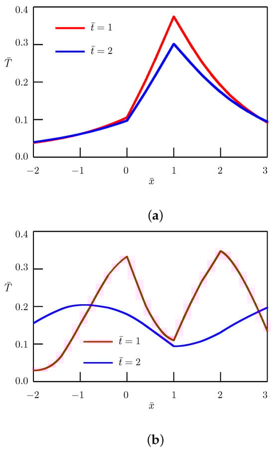
Figure 1.
Fundamental solution to the Cauchy problem. Dependence of temperature on distance for —(a) and —(b).
3. Fundamental Solution to the Source Problem
We solve the time-fractional heat conduction equations
under the zero initial conditions
and under the boundary conditions of nonperfect thermal contact in (12) and (13).
The Laplace integral transform with respet to time t and the Fourier cosine transforms with respect to the spatial coordinates x result in the expressions for temperature in the Laplace transform domain:
Now, we use Equation (36) and the following equation for the inverse Laplace transform: [15,16]
where the Wright function is expressed as [15,16,17,18,19]
In such a way, we arrive at the solution
In the case of ballistic heat conduction (), we have
The dependence of the solution on distance is depicted in Figure 2 and Figure 3 for different values of the order of fractional derivative. In numerical simulations, we have utilized the nondimensional temperatures
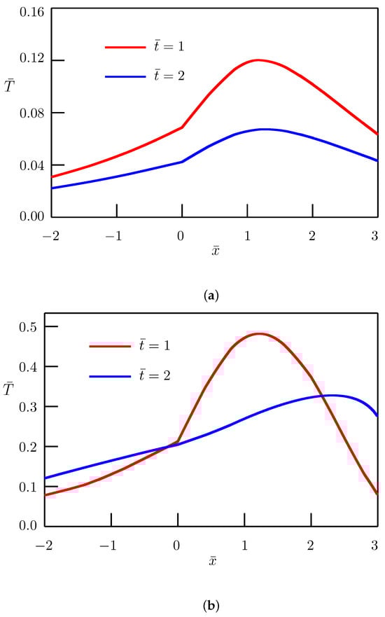
Figure 2.
Fundamental solution to the source problem. Dependence of temperature on distance for —(a), —(b).
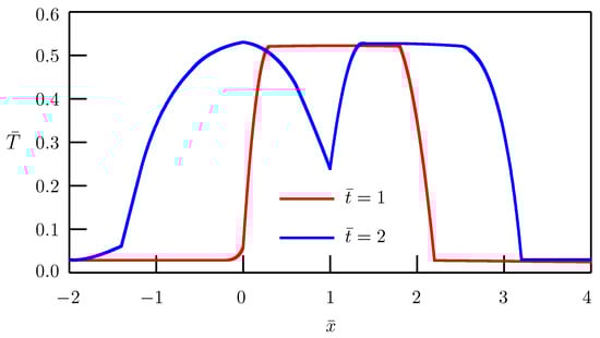
Figure 3.
Fundamental solution to the source problem. Dependence of temperature on distance for .
Other nondimensional quantities are the same as in Equation (46).
4. Concluding Remarks
We have studied the fundamental solutions to the Cauchy problem along with the source problem for time-fractional heat conduction equations in a composite solid under conditions of nonperfect thermal contact. For an arbitrary function describing the initial condition or the source term, the solution can be obtained as a convolution of the corresponding fundamental solution and this function. It should be emphasized that, in the case of classical heat conduction (), the fundamental solutions to the Cauchy problem and to the source problem coincide, whereas, in the case of fractional heat conduction, they are essentially different.
The fundamental solutions were obtained in terms of the generalized Mittag-Leffler, Mainardi, and Wright functions. In numerical simulations, we used the algorithms [20,21] for the calculation of these functions.
For the order of time-fractional derivative , the fractional heat conduction equation interpolates between the elliptic-type Helmholtz equation and the standard heat conduction equation of the parabolic type. When the order of time-fractional derivative , the fractional heat conduction equation interpolates between the classical heat conduction equation and the hyperbolic wave equation. In the instant of ballistic heat conduction (), the wave fronts appear at and for and at , where and can be interpreted as speeds of heat wave propagation in contacting solids. Figure 3 shows how these wave fronts are approximated when the order of fractional derivative approaches 2.
Author Contributions
Conceptualization, Y.P. and T.K.; methodology, Y.P. and T.K.; validation, V.D. and A.Y.; formal analysis, V.D. and A.Y.; investigation, Y.P., T.K., and V.D.; software, T.K. and A.Y.; vizualization, T.K. and A.Y.; supervision, Y.P.; project administrator, Y.P.; writing—original draft preparation, T.K. and A.Y.; writing—review and editing, Y.P. and V.D. All authors have read and agreed to the published version of the manuscript.
Funding
This research received no external funding.
Institutional Review Board Statement
Not applicable.
Data Availability Statement
Data are contained within the article.
Conflicts of Interest
The authors declare no conflicts of interest.
Appendix A. Fractional Integrals and Derivatives
Integral and differential operators of non-integer order are defined as follows [17,19]: the Riemann–Liouville fractional integral:
the Riemann–Liouville fractional derivative:
the Caputo fractional derivative:
Recall the Laplace transform rules for fractional integrals and derivatives:
Here, the asterisk denotes the transform and s is the Laplace transform variable.
References
- Tarasov, V.E. Fractional Dynamics: Applications of Fractional Calculus to Dynamics of Particles, Fields and Media; Higher Education Press: Beijing, China; Springer: Berlin/Heidelberg, Germany, 2010. [Google Scholar]
- Uchaikin, V.V. Fractional Derivatives for Physicists and Engineers; Higher Education Press: Beijing, China; Springer: Berlin/Heidelberg, Germany, 2013. [Google Scholar]
- Atanacković, T.M.; Pilipović, S.; Stanković, B.; Zorica, D. Fractional Calculus with Applications in Mechanics: Vibrations and Diffusion Processes; John Wiley & Sons: Hoboken, NJ, USA, 2014. [Google Scholar]
- Tarasov, V.E. Heat transfer in fractal materials. Int. J. Heat Mass Transf. 2016, 93, 427–430. [Google Scholar] [CrossRef]
- Pagnini, G. Fractional kinetics in random/complex media. In Handbook of Fractional Calculus with Applications, Volume 5: Applications in Physics, Part B; De Gruyter: Berlin, Germany, 2019; pp. 183–205. [Google Scholar]
- Zhmakin, A.I. Heat conduction beyond the Fourier law. Techn. Phys. 2021, 66, 1–22. [Google Scholar] [CrossRef]
- Zhmakin, A.I. Non-Fourier Heat Conduction: From Phase-Lag Models to Relativistic and Quantum Transport; Springer: Berlin/Heidelberg, Germany, 2023. [Google Scholar]
- Zhou, Y. Fractional Diffusion and Wave Equations: Well-Posedness and Inverse Problems; Springer: Cham, Switzerland, 2024. [Google Scholar]
- Povstenko, Y. Fractional Thermoelasticity, 2nd ed.; Springer: Berlin/Heidelberg, Germany, 2024. [Google Scholar]
- Kharrat, M.; Touafek, N.; Krichen, M. (Eds.) Modeling of Discrete and Continuous Systems: Ordinary, Partial and Fractional Derivatives; Springer: Singapore, 2025. [Google Scholar]
- Povstenko, Y.; Kyrylych, T. Fractional heat conduction in solids connected by thin intermediate layer: Nonperfect thermal contact. Continuum Mech. Thermodyn. 2019, 31, 1719–1731. [Google Scholar] [CrossRef]
- Podstrigach, Y.S. Temperature field in a system of solids conjugated by a thin intermediate layer. Inzh. Fiz. Zhurn. 1963, 6, 129–136. (In Russian) [Google Scholar]
- Povstenko, Y. Fractional heat conduction in infinite one-dimensional composite medium. J. Therm. Stress. 2013, 36, 351–363. [Google Scholar] [CrossRef]
- Prudnikov, A.P.; Brychkov, Y.A.; Marichev, O.I. Integrals and Series, Volume 1: Elementary Functions; Gordon and Breach Science Publishers: Amsterdam, The Netherlands, 1986. [Google Scholar]
- Mainardi, F. The fundamental solutions for the fractional diffusion-wave equation. Appl. Math. Lett. 1996, 9, 23–28. [Google Scholar] [CrossRef]
- Mainardi, F. Fractional relaxation-oscillation and fractional diffusion-wave phenomena. Chaos Solitons Fractals 1996, 7, 1461–1477. [Google Scholar] [CrossRef]
- Podlubny, I. Fractional Differential Equations; Academic Press: San Diego, CA, USA, 1999. [Google Scholar]
- Gorenflo, R.; Kilbas, A.A.; Mainardi, F.; Rogosin, S.V. Mittag-Leffler Functions, Related Topics and Applications, 2nd ed.; Springer: Berlin/Heidelberg, Germany, 2020. [Google Scholar]
- Kilbas, A.A.; Srivastava, H.M.; Trujillo, J.J. Theory and Applications of Fractional Differential Equations; Elsevier: Amsterdam, The Netherlands, 2006. [Google Scholar]
- Gorenflo, R.; Loutchko, J.; Luchko, Y. Computation of the Mittag-Leffler function Eα,β(z) and its derivatives. Fract. Calc. Appl. Anal. 2002, 5, 491–518, Erratum in Fract. Calc. Appl. Anal. 2003, 6, 111–112. [Google Scholar]
- Luchko, Y. Algorithms for evaluation of the Wright function for the real arguments’ values. Fract. Calc. Appl. Anal. 2008, 11, 57–75. [Google Scholar]


Disclaimer/Publisher’s Note: The statements, opinions and data contained in all publications are solely those of the individual author(s) and contributor(s) and not of MDPI and/or the editor(s). MDPI and/or the editor(s) disclaim responsibility for any injury to people or property resulting from any ideas, methods, instructions or products referred to in the content. |
© 2025 by the authors. Licensee MDPI, Basel, Switzerland. This article is an open access article distributed under the terms and conditions of the Creative Commons Attribution (CC BY) license (https://creativecommons.org/licenses/by/4.0/).