Simulation-Based Two-Stage Scheduling Optimization Method for Carrier-Based Aircraft Launch and Departure Operations


Abstract
1. Introduction
2. Problem Description and Modeling
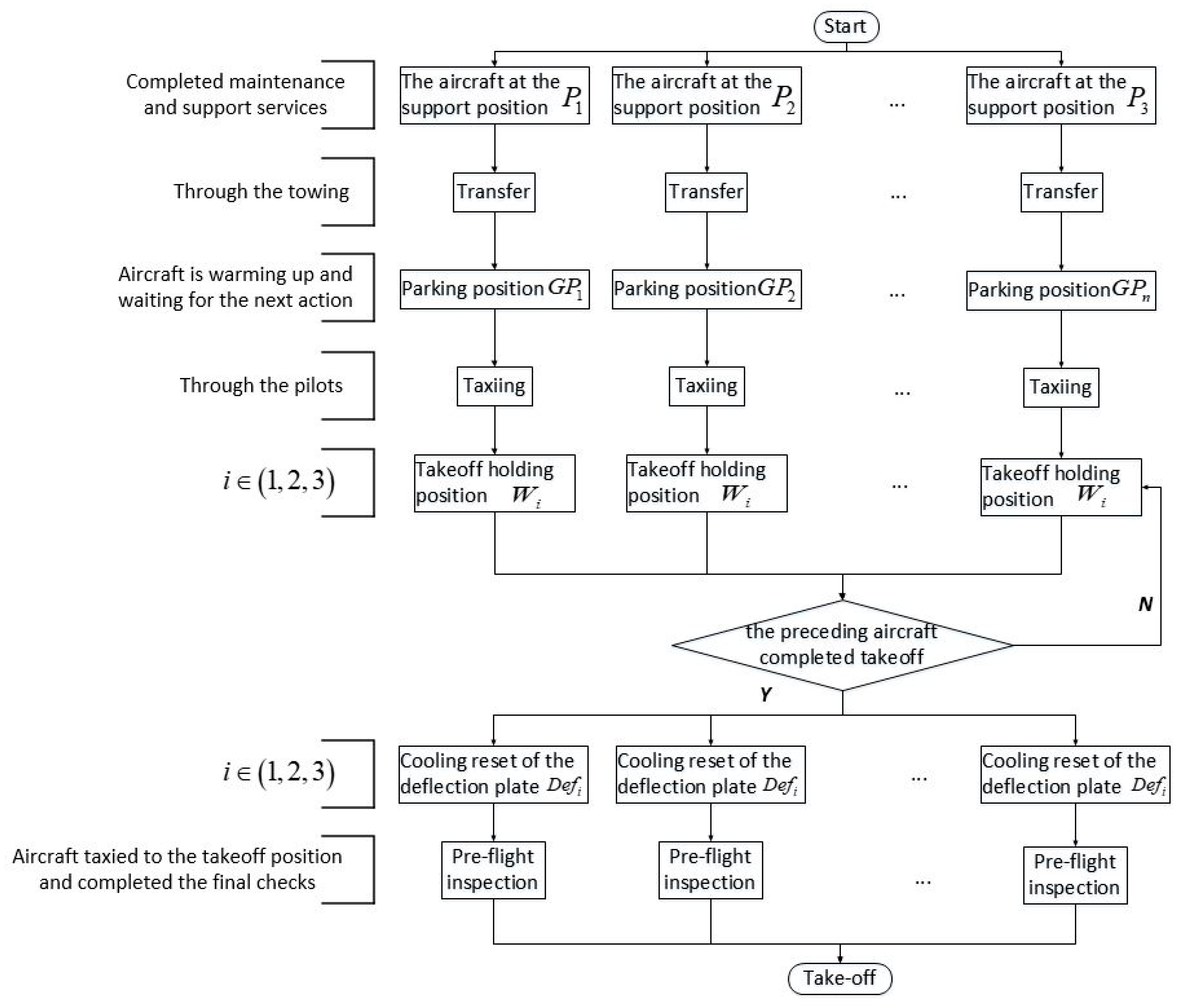
2.1. Problem Description
2.1.1. Aircraft–Position Matching
2.1.2. Aircraft Transfer and Taxiing
2.1.3. Jet Blast Deflector (JBD) Cooling and Reset
2.1.4. Preflight Inspection
2.1.5. Takeoff and Departure
2.2. Notation
- Indices
- Sets
- Parameter
- Decision variables
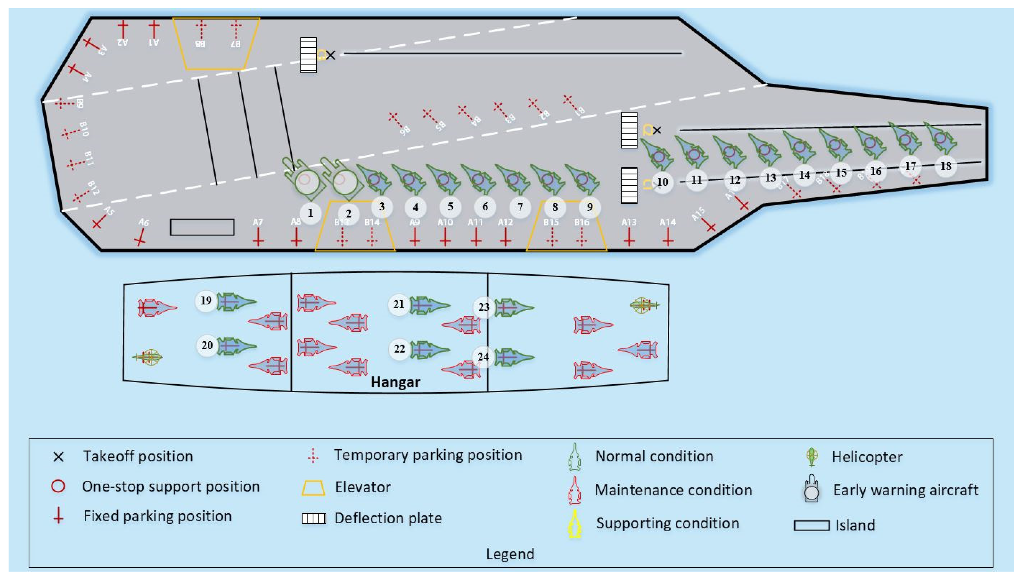
2.3. Simulation Model Development for Carrier-Based Aircraft Departure Operations
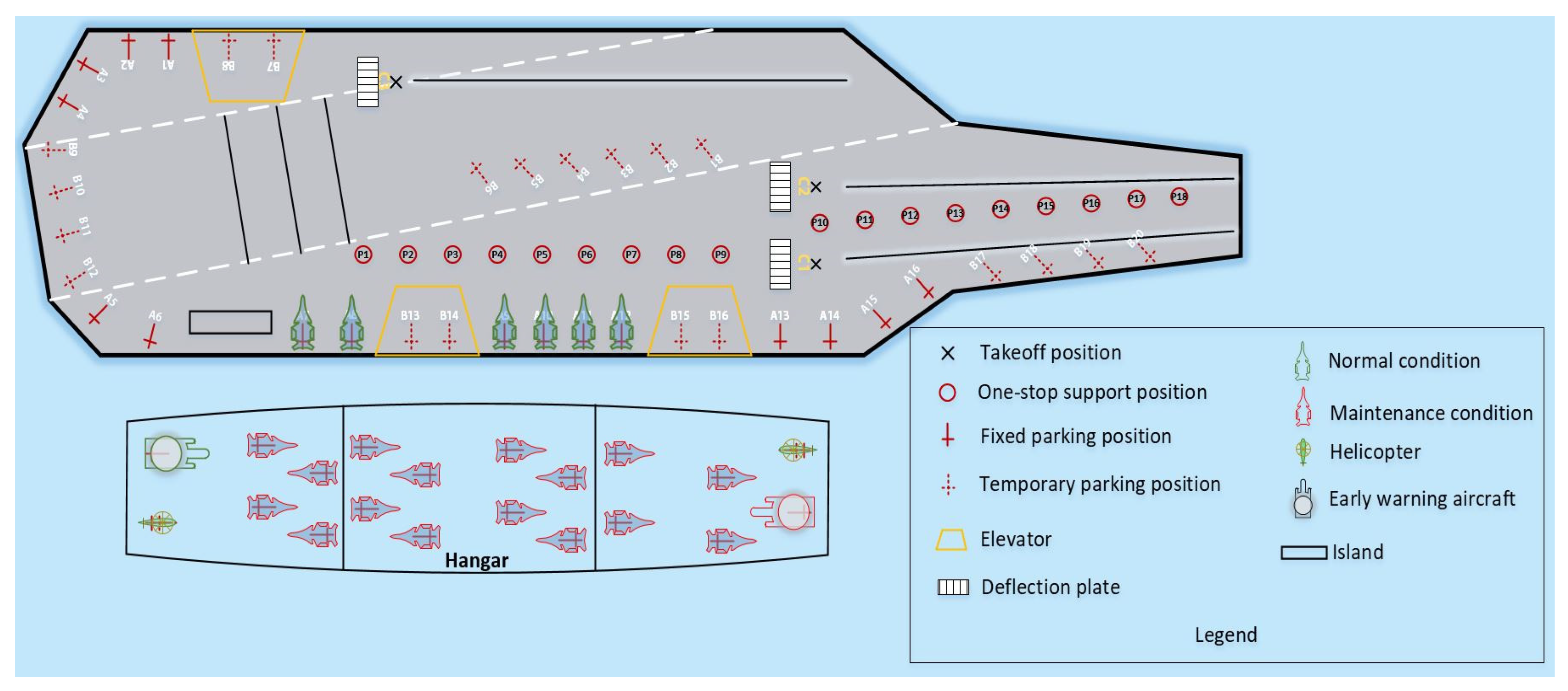
2.3.1. Environmental Resource Modeling
2.3.2. Collision Detection System
2.4. Collision Avoidance Strategies for Multi-Aircraft Coordination
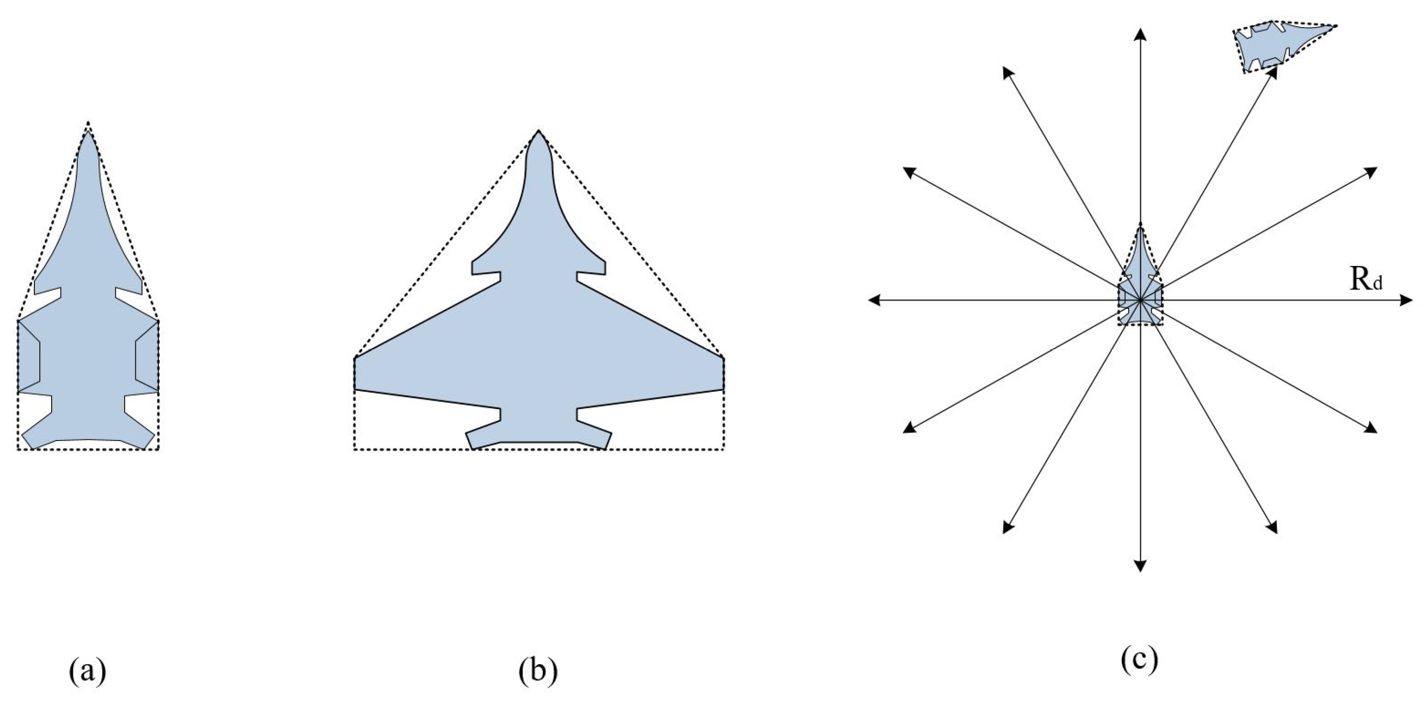
2.4.1. Basal Path Selection Protocol
- Geo-spatial way-points (x, y coordinates);
- Orientation angles at critical maneuvering nodes;
- Temporal sequencing between consecutive way-points;
- Velocity modulation patterns across path segments;
- Integrated metrics for path length and execution duration.
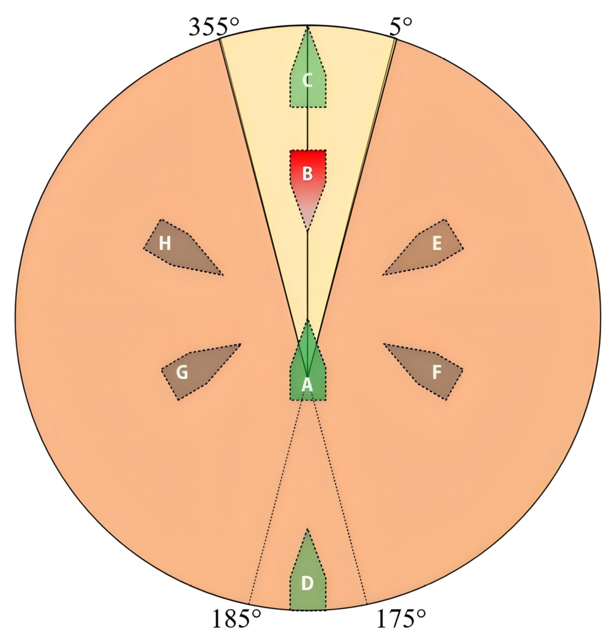
2.4.2. Collision Avoidance Strategies for Aircraft Encounters
- (a)
- Following scenario (A → C/D in Figure 4)
- (b)
- Head-on scenario (A → B in Figure 4)
- (c)
- Crossing scenario (A → E/F/G/H in Figure 4)
- Mandatory velocity reduction
- Differential steering governed by Equations (4) and (5):
2.4.3. Obstacle Avoidance Protocol
- (1).
- When the aircraft is located within the port-side area of the deck (), with its coordinate being , its collision avoidance strategy is determined based on Equation (6).
- (2).
- When the aircraft is located within the starboard-side area of the deck (), with its coordinate being , its collision avoidance strategy is determined based on Equations (7).
- (3).
- When the carrier-based aircraft is in the deck landing area (), it will not collide with any physical boundary on the deck. Therefore, its motion remains unchanged as expressed in Equations (8).
- (4).
- When the obstacle () is not a deck entity boundary and is located in the port-side area of the deck, then it satisfies the following expression:
- (5).
- When the obstacle () is not a deck entity boundary and is located in the starboard area of the deck, then it satisfies the following expression:
- (6).
- When the obstacle is not a deck entity boundary and is located within the landing area of the deck, the judgment should be made based on the relative distance between the current aircraft () and the encountered aircraft (), as expressed in Equation (9).
2.4.4. Dynamic Priority Assignment
- Definition of initial priority
- Definition of dynamic priority
2.4.5. Rescheduling Protocol
- Priority-driven re-queuing: Aircrafts with lower priority are re-queued according to the established hierarchy, resetting their scheduling sequence to the terminal position.
- Conflict flagging: Higher-priority aircrafts maintain operational continuity while receiving conflict markers (denoted by ) for trajectory re-calibration.
2.5. Two-Stage Scheduling Optimization Framework for Aircraft Departure Operations
- (1)
- Non-interruptible process: Departure operations proceed without suspension.
- (2)
- Predetermined positional states: Deployment coordinates for aircraft and support/parking/launch positions are predefined.
- (3)
- Persistent operational readiness: All equipment maintain baseline functionality throughout operations.
- (4)
- Exclusive tractor assignment: Each tractor tows a single aircraft with independent workflows.
- (5)
- Aircraft-specific timing: Warm-up, wake separation, and pre-launch durations are type-dependent constants.
3. Design of a Two-Stage Scheduling Model Solving Algorithm for Carrier-Based Aircraft Departure Operations
- (1)
- Aircraft parking position assignment;
- (2)
- Take-off station selection;
- (3)
- Take-off sequence determination;
3.1. Design of AAE–SAC Algorithm
3.1.1. Design of State Space, Action Space, and Reward Function
3.1.2. Dynamic Target Entropy and Attention Mechanism
| Algorithm 1. Attentive Adaptive Entropy SAC (AAE–SAC) Algorithm |
| Require: Number of aircraft: , , , , Ensure: , Learned Q-functions: 1: Initialize networks: 2: 3: 4: 5: 6: for episode to do 7: 8: do 9: Compute attention weights: 10: Apply attention: 11: Select action: 12: 13: Compute reward components: 14: in 15: if update time then 16: Sample batch from 17: Compute target Q-values: 18: Update critics: 19: Update policy: 20: Update temperature: 21: end if 22: end for 23: end for 24: return |
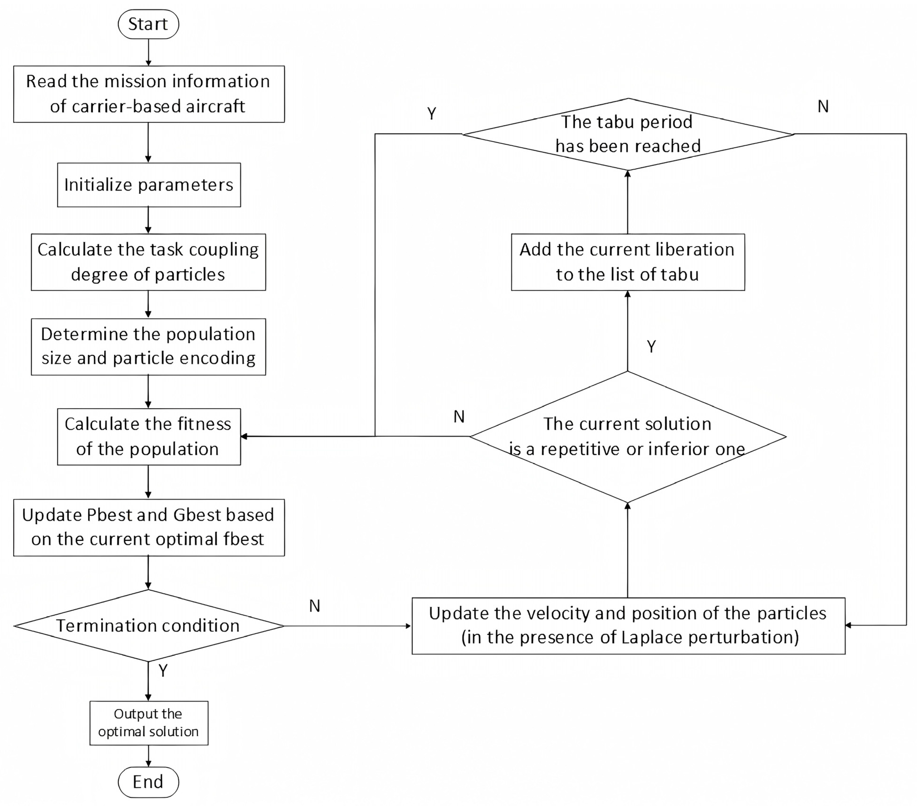
3.2. Design of LTA-HPSO Algorithm
3.2.1. Particle Swarm Coding and Decoding
3.2.2. Population Division
3.2.3. Fitness Function
3.2.4. Update Mechanism
| Algorithm 2. Laplacian–Tabu Augmented Hierarchical PSO (LTA-HPSO) Algorithm |
| Require: Number of aircraft: Number of parking positions: Number of departure positions: Ensure: Optimal parking position selection and departure order: Minimum fitness value: 1: Initialize population for all particles 2: Initialize 3: 4: for do 5: for each particle in the population do 6: using Laplacian perturbation: 7: : 8: : 9: if then 10: 11: 12: end if 13: end for 14: Update penalty coefficient : 15: Update inertia weight : 16: Update Laplacian scale parameter : 17: Update tabu table: 18: if then 19: to tabu table 20: end if 21: end for 22: return |
3.3. Summary of Solution Methods
4. Simulation Experiment and Result Analysis
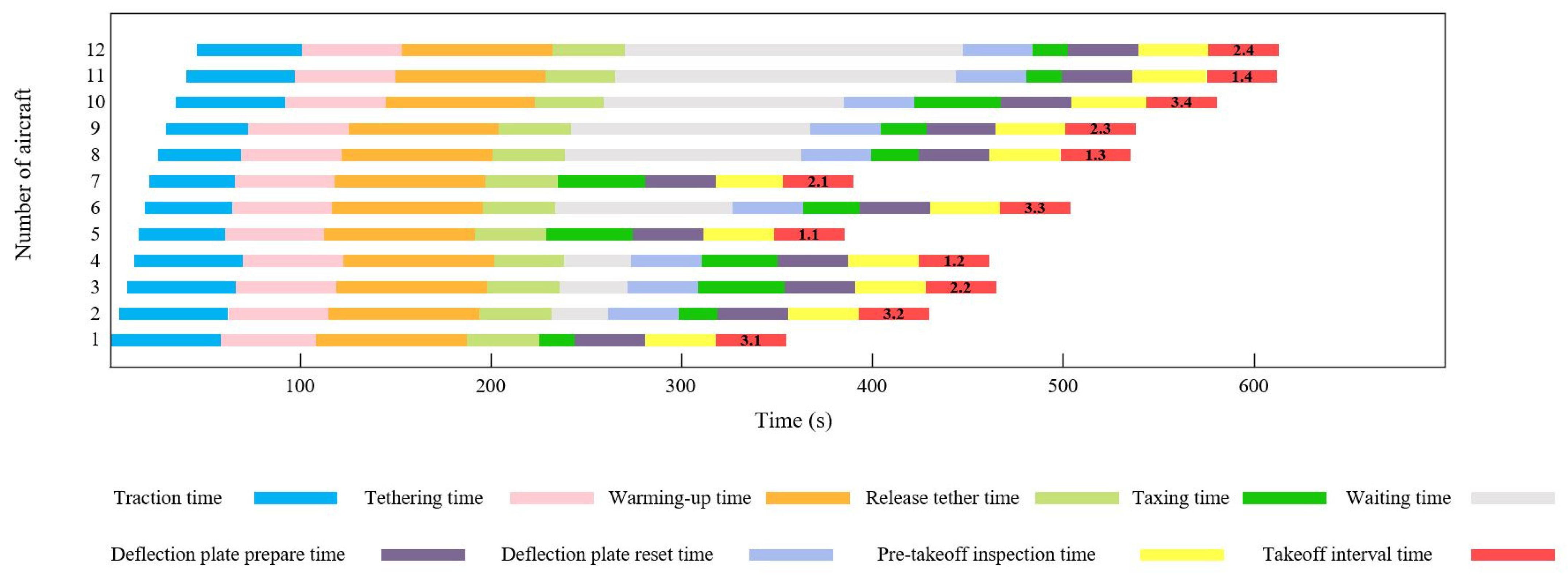
4.1. Case 1
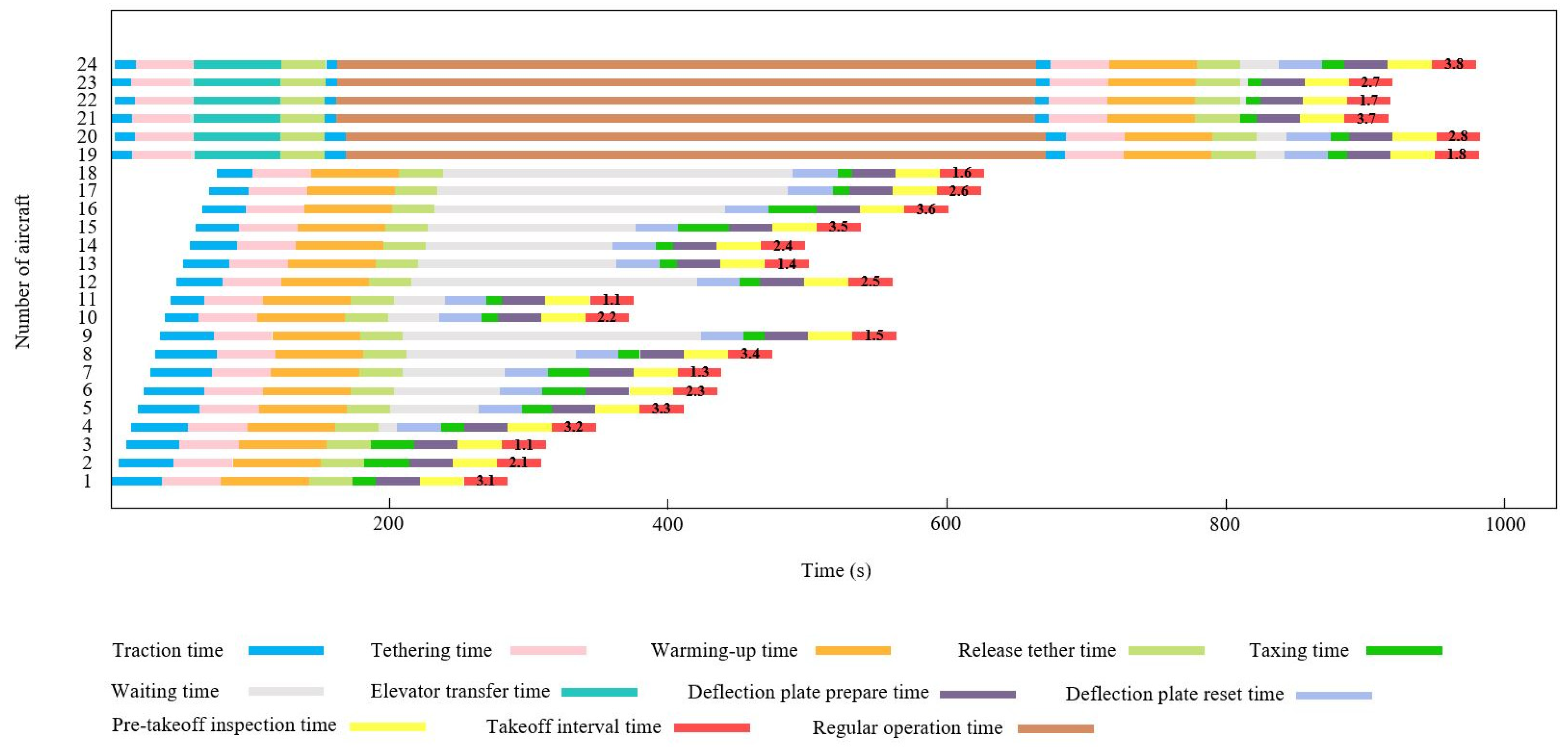
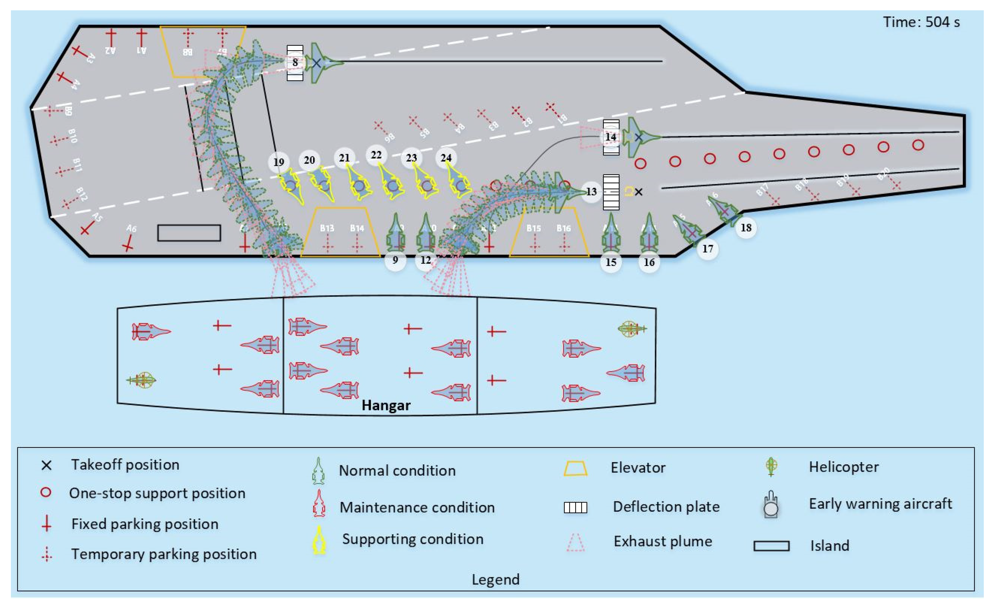
4.2. Case 2
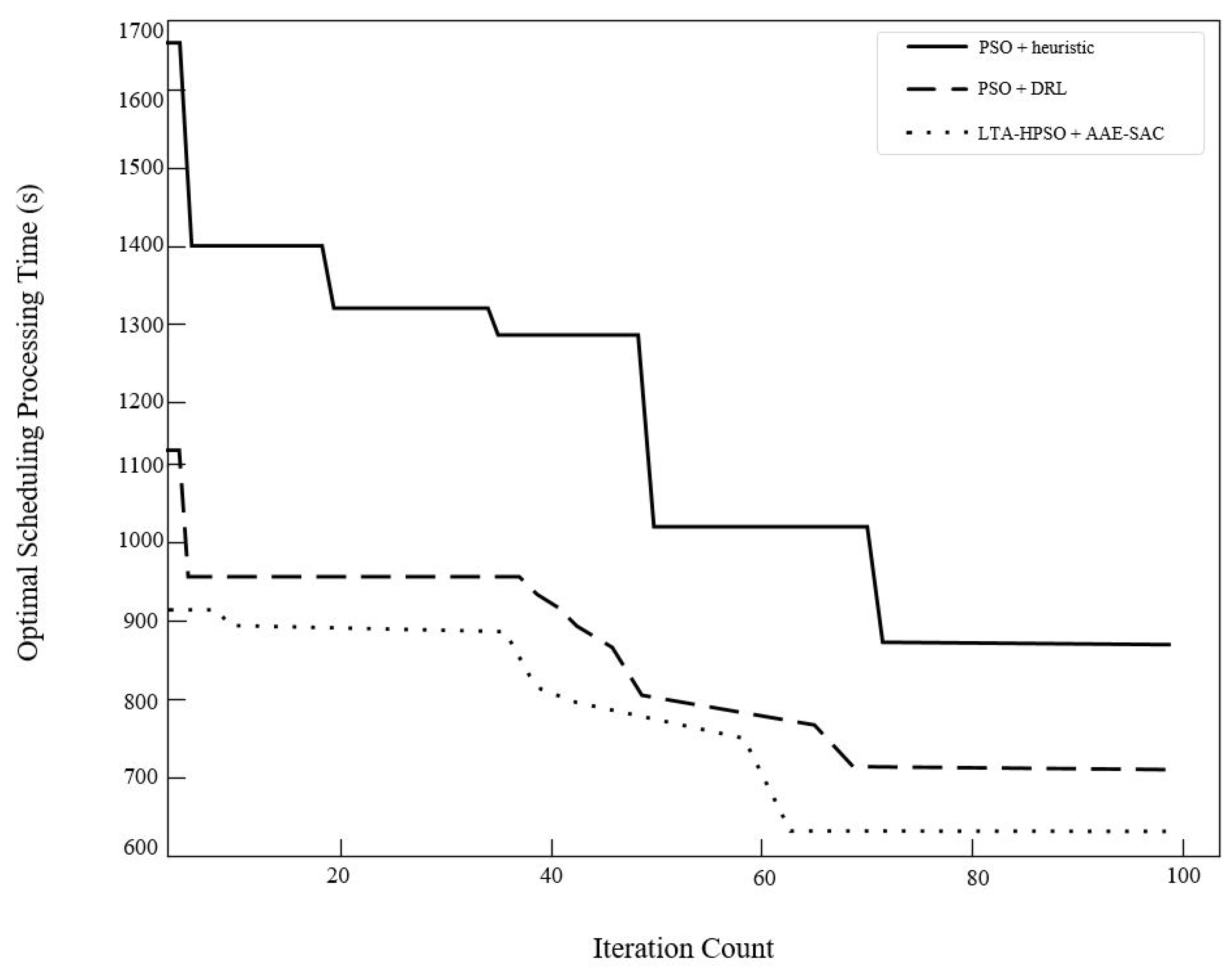
4.3. Analysis of Algorithm Performance
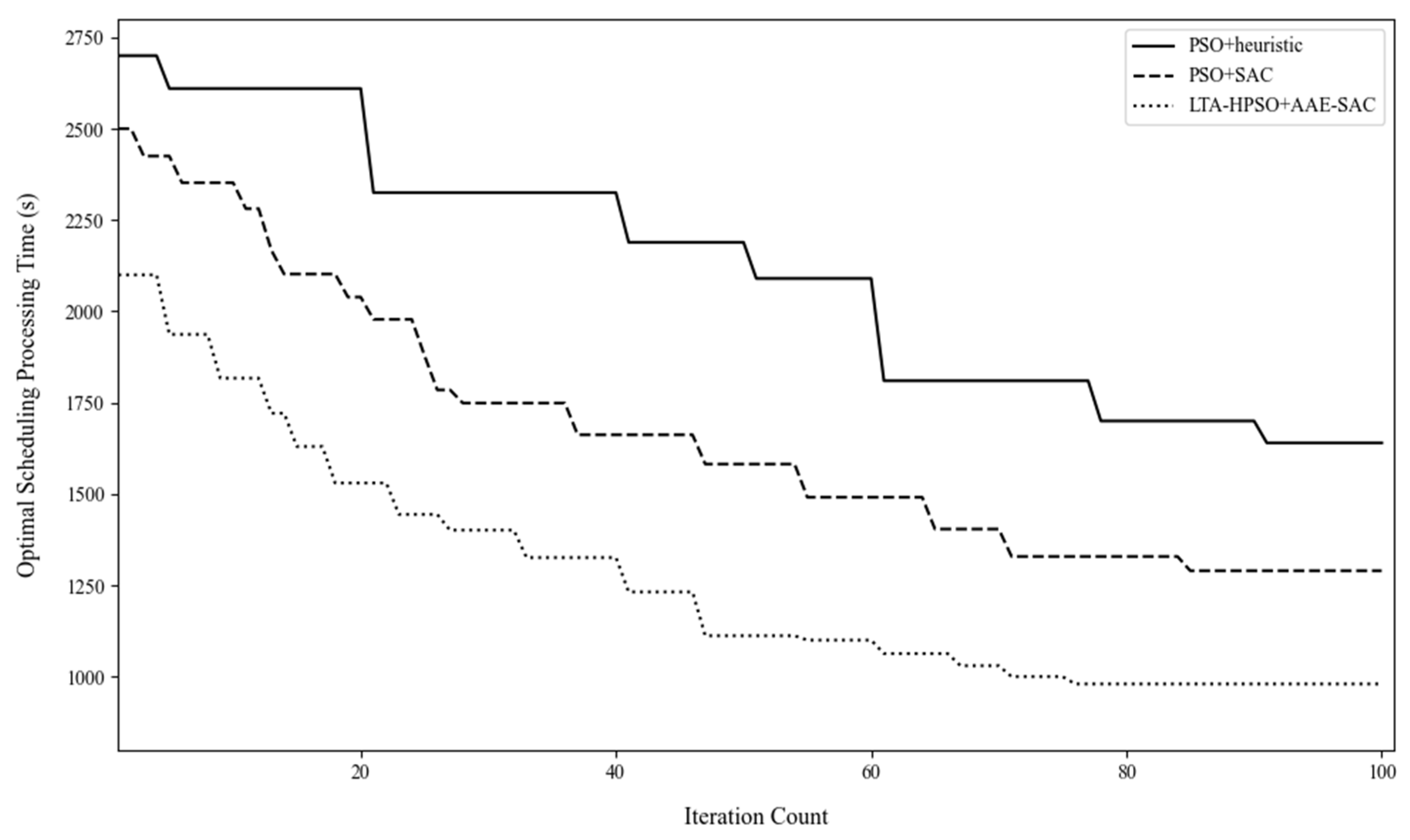
4.3.1. Algorithm Comparison
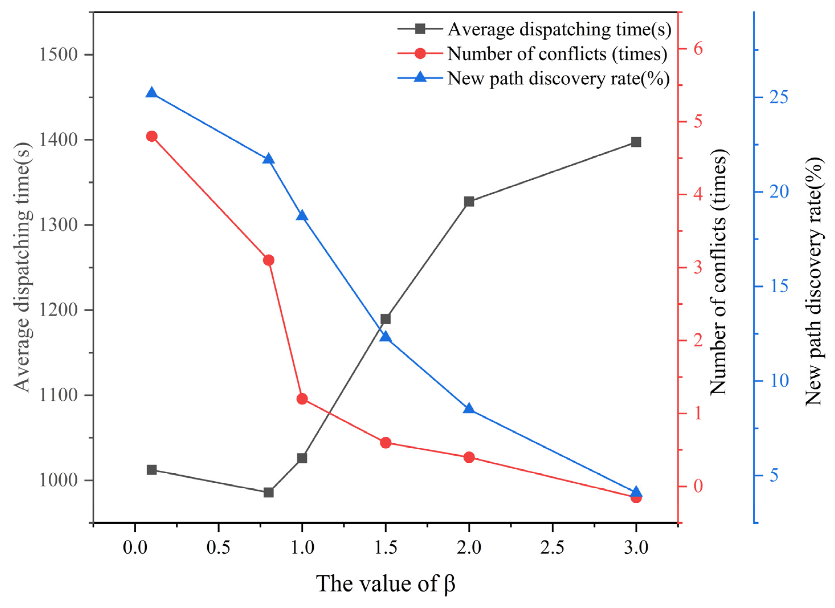
4.3.2. Sensitivity Analysis
5. Conclusions
Author Contributions
Funding
Institutional Review Board Statement
Data Availability Statement
Conflicts of Interest
References
- Wei, M.; Yang, S.; Wu, W.; Sun, B. A multi-objective fuzzy optimization model for multi-type aircraft flight scheduling problem. Transport 2024, 39, 313–322. [Google Scholar] [CrossRef]
- Sun, B.; Xu, Z.; Wei, M.; Wang, X. A study on the strategic behavior of players participating in air-rail intermodal transportation based on evolutionary games. J. Air Transp. Manag. 2025, 126, 102793. [Google Scholar] [CrossRef]
- Jewell, A.; Wigge, M.A.; Gagnon, C.M.; Lynn, L.A.; Kirk, K.M.; Berg, K.K.; Roberts, T.A.; Hale, A.J.; Jones, W.L.; Matheny, A.M.; et al. USS Nimitz and Carrier Airwing Nine Surge Demonstration; Center for Naval Analyses: Alexandria, Egypt, 1998. [Google Scholar]
- Michels, A.S.; Thate, T. Requirements for Digitized Aircraft Spotting (Ouija) Board for Use on US Navy Aircraft Carriers; Naval Postgraduate School: Monterey, CA, USA, 2002. [Google Scholar]
- US Navy Air Systems Command. Navy Training System Plan for Aviation Data Management and Control System. US Navy. 2002. Available online: https://www.globalsecurity.org/military/library/policy/navy/ntsp/admacs-a_2002.pdf (accessed on 20 May 2025).
- Zhang, Z.; Lin, S.; Dong, R.; Zhu, Q. Designing a Human-Computer Cooperation Decision Planning System for Aircraft Carrier Deck Scheduling. In Proceedings of the AIAA Infotech@ Aerospace, Kissimmee, FL, USA, 5–9 January 2015; p. 1111. [Google Scholar]
- Ryan, J.; Cummings, M.; Roy, N.; Banerjee, A.; Schulte, A. Designing an Interactive Local and Global Decision Support System for Aircraft Carrier Deck Scheduling. In Proceedings of the Infotech@ Aerospace 2011, St. Louis, MO, USA, 29–31 March 2011; p. 1516. [Google Scholar]
- Ghosh Dastidar, R.; Frazzoli, E. A Queueing Network Based Approach to Distributed Aircraft Carrier Deck Scheduling. In Proceedings of the Infotech@ Aerospace 2011, St. Louis, MO, USA, 29–31 March 2011; p. 1514. [Google Scholar]
- Michini, B.; How, J. A Human-Interactive Course of Action Planner for Aircraft Carrier Deck Operations. In Proceedings of the Infotech@ Aerospace 2011, St. Louis, MO, USA, 29–31 March 2011; p. 1515. [Google Scholar]
- Yuan, P.; Han, W.; Su, X.; Liu, J.; Song, J. A Dynamic Scheduling Method for Carrier Aircraft Support Operation Under Uncertain Conditions Based on Rolling Horizon Strategy. Appl. Sci. 2018, 8, 1546. [Google Scholar] [CrossRef]
- Wan, B.; Han, W.; Su, X.C.; Liu, J. Carrier-Based Aircraft Departure Scheduling Optimization Based on CE-PF Algorithm. J. Beijing Univ. Aeronaut. Astronaut. 2022, 48, 771–785. (In Chinese) [Google Scholar]
- Liu, Z.X.; Wan, B.; Su, X.C.; Guo, F.; Liu, Y.J. Sortie Scheduling Method of Carrier Aircraft Based on HA Algorithm. Syst. Eng. Electron. 2024, 46, 1691–1702. (In Chinese) [Google Scholar]
- Wang, H.; Jiang, Z.; Wang, Y.; Zhang, H.; Wang, Y. A two-stage optimization method for energy-saving flexible job-shop scheduling based on energy dynamic characterization. J. Clean. Prod. 2018, 192, 534–546. [Google Scholar] [CrossRef]
- Si, W.; Sun, T.; Song, C.; Zhang, J. Design and Verification of a Transfer Path Optimization Method for an Aircraft on the Aircraft Carrier Flight Deck. Front. Inf. Technol. Electron. Eng. 2021, 22, 1221–1233. [Google Scholar] [CrossRef]
- Li, H.; Zhu, Y.; Chen, Y.; Pedrielli, G.; Pujowidianto, N.A. The Object-Oriented Discrete Event Simulation Modeling: A Case Study on Aircraft Spare Part Management. In Proceedings of the 2015 Winter Simulation Conference (WSC), Huntington Beach, CA, USA, 6–9 December 2015. [Google Scholar]
- McWhite, J.D. CVNX—Expanded Capability Baseline Aircraft Carrier Design Study. Nav. Eng. J. 2000, 112, 47–57. [Google Scholar] [CrossRef]
- Nemirko, A.P.; Dulá, J.H. Machine Learning Algorithm Based on Convex Hull Analysis. Procedia Comput. Sci. 2021, 186, 381–386. [Google Scholar] [CrossRef]
- Jiang, L.; Fang, D.J.; Zhou, H.W.; Huang, H.B. Improved Global Path Planning Algorithm Based on Ray Model. Acta Electron. Sin. 2022, 50, 548–556. (In Chinese) [Google Scholar]
- Liu, J. Research on Path Planning for Carrier-Based Aircraft Tractor Based on Inverse Reinforcement Learning. Master’s Thesis, Harbin Engineering University, Harbin, China, 2017. [Google Scholar]
- Meng, S.; Zhu, Q.; Xia, F. Improvement of the Dynamic Priority Scheduling Algorithm Based on a Heapsort. IEEE Access 2019, 7, 68503–68510. [Google Scholar] [CrossRef]
- Tian, B.; Xiao, G.; Shen, Y. A deep reinforcement learning approach for dynamic task scheduling of flight tests. J. Supercomput. 2024, 80, 18761–18796. [Google Scholar] [CrossRef]
- Wu, Y.; Hu, N.; Qu, X. A General Trajectory Optimization Method for Aircraft Taxiing on Flight Deck of Carrier. Proc. Inst. Mech. Eng. Pt. G. J. Aerosp. Eng. 2019, 233, 1340–1353. [Google Scholar] [CrossRef]
- Christiano, P.F.; Leike, J.; Brown, T.; Martic, M.; Legg, S.; Amodei, D. Deep reinforcement learning from human preferences. Adv. Neural Inf. Process. Syst. 2017, 30, 4302–4310. [Google Scholar]
- Li, F.; Lang, S.; Hong, B.; Reggelin, T. A two-stage RNN-based deep reinforcement learning approach for solving the parallel machine scheduling problem with due dates and family setups. J. Intell. Manuf. 2024, 35, 1107–1140. [Google Scholar] [CrossRef]
- Yan, Q.; Wang, H.; Wu, F. Digital Twin-Enabled Dynamic Scheduling with Preventive Maintenance Using a Double-Layer Q-Learning Algorithm. Comput. Oper. Res. 2022, 144, 105823. [Google Scholar] [CrossRef]
- Wang, Z.; Cai, B.; Li, J.; Yang, D.; Zhao, Y.; Xie, H. Solving Non-Permutation Flow-Shop Scheduling Problem via a Novel Deep Reinforcement Learning Approach. Comput. Oper. Res. 2023, 151, 106095. [Google Scholar] [CrossRef]
- Wong, M.F.; Tan, C.W. Aligning Crowd-Sourced Human Feedback for Reinforcement Learning on Code Generation by Large Language Models. IEEE Trans. Big Data 2024. [Google Scholar] [CrossRef]
- Zhang, Y.; Zhu, H.; Tang, D. An Improved Hybrid Particle Swarm Optimization for Multi-Objective Flexible Job-Shop Scheduling Problem. Kybernetes 2020, 49, 2873–2892. [Google Scholar] [CrossRef]
- Liu, L.L.; Hu, R.S.; Hu, X.P.; Zhao, G.P.; Wang, S. A Hybrid PSO-GA Algorithm for Job Shop Scheduling in Machine Tool Production. Int. J. Prod. Res. 2015, 53, 5755–5781. [Google Scholar] [CrossRef]
- Ding, H.; Gu, X. Improved Particle Swarm Optimization Algorithm Based Novel Encoding and Decoding Schemes for Flexible Job Shop Scheduling Problem. Comput. Oper. Res. 2020, 121, 104951. [Google Scholar] [CrossRef]
- Vakanski, A.; Mantegh, I.; Irish, A.; Janabi-Sharifi, F. Trajectory Learning for Robot Programming by Demonstration Using Hidden Markov Model and Dynamic Time Warping. IEEE Trans. Syst. Man Cybern. Part B (Cybern.) 2012, 42, 1039–1052. [Google Scholar] [CrossRef] [PubMed]
- Giorgino, T. Computing and Visualizing Dynamic Time Warping Alignments in R: The dtw Package. J. Stat. Softw. 2009, 31, 1–24. [Google Scholar] [CrossRef]
- Boularias, A.; Kober, J.; Peters, J. Relative Entropy Inverse Reinforcement Learning. Proc. Fourteenth Int. Conf. Artif. Intell. Stat. 2011, 15, 182–189. [Google Scholar]
- Nica, A.; Khetarpal, K.; Precup, D. The Paradox of Choice: Using Attention in Hierarchical Reinforcement Learning. arXiv 2022, arXiv:2201.09653. Available online: https://arxiv.org/abs/2201.09653 (accessed on 20 May 2025).
- Xia, G.; Luan, T.; Sun, M. Evaluation Analysis for Sortie Generation of Carrier Aircrafts Based on Nonlinear Fuzzy Matter-Element Method. J. Intell. Fuzzy Syst. 2016, 31, 3055–3066. [Google Scholar] [CrossRef]
- Fujimoto, S.; Hoof, H.; Meger, D. Addressing Function Approximation Error in Actor-Critic Methods. Int. Conf. Mach. Learn. 2018, 80, 1587–1596. [Google Scholar]
- Zhang, X.; Guo, P.; Zhang, H.; Yao, J. Hybrid Particle Swarm Optimization Algorithm for Process Planning. Mathematics 2020, 8, 1745. [Google Scholar] [CrossRef]
- Kuo, R.J.; Syu, Y.J.; Chen, Z.Y.; Tien, F.C. Integration of Particle Swarm Optimization and Genetic Algorithm for Dynamic Clustering. Inf. Sci. 2012, 195, 124–140. [Google Scholar] [CrossRef]
- Pant, M.; Thangaraj, R.; Abraham, A.; Grosan, C. Differential Evolution with Laplace Mutation Operator. 2009 IEEE Congr. Evol. Comput. 2009, 2841–2849. [Google Scholar]
- Peng, C.; Wu, G.; Liao, T.W.; Wang, H. Research on Multi-Agent Genetic Algorithm Based on Tabu Search for the Job Shop Scheduling Problem. PLoS ONE 2019, 14, e0223182. [Google Scholar] [CrossRef] [PubMed]


| Type of Aircraft | Priority Rank | Type of Mission | Priority Rank | ||
|---|---|---|---|---|---|
| Early-warning aircraft | I | 3 | Ground strike | I | 3 |
| Heavy aircraft | II | 2 | Air-to-air | II | 2 |
| Stealth/electronic aircraft | III | 1 | Cruise | III | 1 |
| Parameter Name | Value |
|---|---|
| Population size | 100 |
| Maximum number of iterations | 100 |
| 0.5 | |
| 0.5 | |
| 1.2 | |
| 0.15 |
| Parameter Name | Values and Units | Parameter Name | Values and Units |
|---|---|---|---|
| Landing Gear Retention Time for Aircraft | 40 s | Preparation Time for Bend Plate | 30 s |
| Release Time for Landing Gear of Aircraft | 30 s | Cooling and Reset Time for Bend Plate | 30 s |
| Maximum Traction Speed | 1.5 m/s | Pre-Takeoff Inspection Time | 30 s |
| Maximum Taxiing Speed | 3.0 m/s | Interval Time of take-off | 30 s |
| Transport Time for Lifting Gear | 60 s | Engine Warm-Up Time | 60 s |
| One-stop Support Time | 8 min |
| Number of Algorithm Executions | PSO + Heuristic | PSO + SAC | LTA-HPSO + AAE–SAC | |||
|---|---|---|---|---|---|---|
| Optimal Solution Scheduling Time/s | Algorithm Running Time/s | Optimal Solution Scheduling Time/s | Algorithm Running Time/s | Optimal Solution Scheduling Time/s | Algorithm Running Time/s | |
| Ex1 | 841 | 38.64 | 709 | 157.64 | 692 | 136.56 |
| Ex2 | 870 | 79.87 | 734 | 150.87 | 635 | 115.85 |
| Ex3 | 848 | 68.65 | 706 | 119.84 | 699 | 134.05 |
| Ex4 | 815 | 15.36 | 768 | 200.63 | 661 | 128.72 |
| Ex5 | 864 | 64.62 | 811 | 271.58 | 716 | 143.21 |
| Ex6 | 844 | 34.35 | 738 | 162.23 | 625 | 108.46 |
| Ex7 | 1663 | 129.25 | 835 | 256.83 | 653 | 140.84 |
| Ex8 | 868 | 69.35 | 792 | 223.59 | 622 | 126.23 |
| Ex9 | 1066 | 96.62 | 710 | 122.68 | 609 | 102.63 |
| Ex10 | 816 | 21.44 | 763 | 133.65 | 614 | 114.42 |
| Aircraft Number | Priority | Parking Position Number | Take-Off Position Number | Take-Off Sequence |
|---|---|---|---|---|
| 1 | 3 | A2 | C3 | 1 |
| 2 | 3 | A1 | C3 | 4 |
| 3 | 3 | B8 | C2 | 6 |
| 4 | 3 | B7 | C1 | 5 |
| 5 | 3 | B13 | C1 | 2 |
| 6 | 3 | B14 | C3 | 7 |
| 7 | 3 | A9 | C2 | 3 |
| 8 | 3 | A10 | C1 | 8 |
| 9 | 3 | A11 | C2 | 9 |
| 10 | 3 | A12 | C3 | 10 |
| 11 | 3 | B15 | C1 | 11 |
| 12 | 3 | B16 | C2 | 12 |
| Number of Algorithm Executions | PSO + Heuristic | PSO + SAC | LTA-HPSO + AAE–SAC | |||
|---|---|---|---|---|---|---|
| Optimal Solution Scheduling Time/s | Algorithm Running Time/s | Optimal Solution Scheduling Time/s | Algorithm Running Time/s | Optimal Solution Scheduling Time/s | Algorithm Running Time/s | |
| Ex1 | 2013 | 635.187 | 1354 | 365.354 | 991 | 193.820 |
| Ex2 | 2251 | 678.534 | 1314 | 354.581 | 985 | 201.801 |
| Ex3 | 2595 | 751.684 | 1473 | 439.950 | 984 | 176.725 |
| Ex4 | 1743 | 594.953 | 1311 | 355.315 | 1062 | 214.395 |
| Ex5 | 1976 | 628.512 | 1387 | 412.790 | 995 | 191.963 |
| Ex6 | 2639 | 819.926 | 1293 | 349.201 | 1010 | 205.662 |
| Ex7 | 1640 | 583.541 | 1554 | 437.165 | 1076 | 186.946 |
| Ex8 | 1797 | 581.664 | 1391 | 381.300 | 1093 | 234.839 |
| Ex9 | 1951 | 679.224 | 1606 | 540.937 | 988 | 166.274 |
| Ex10 | 1874 | 597.821 | 1332 | 414.956 | 1074 | 189.460 |
| Aircraft Number | Priority | Parking Position Number | Take-Off Position Number | Take-Off Sequence |
|---|---|---|---|---|
| 1 | 5 | A4 | C3 | 1 |
| 2 | 5 | A3 | C2 | 2 |
| 3 | 3 | A2 | C1 | 3 |
| 4 | 3 | A1 | C3 | 4 |
| 5 | 3 | A5 | C3 | 7 |
| 6 | 3 | A6 | C2 | 8 |
| 7 | 3 | A7 | C1 | 9 |
| 8 | 3 | A8 | C3 | 10 |
| 9 | 3 | A9 | C1 | 15 |
| 10 | 4 | B2 | C2 | 5 |
| 11 | 4 | B1 | C1 | 6 |
| 12 | 3 | A10 | C2 | 14 |
| 13 | 3 | A11 | C1 | 12 |
| 14 | 3 | A12 | C2 | 11 |
| 15 | 3 | A13 | C3 | 13 |
| 16 | 3 | A14 | C3 | 16 |
| 17 | 3 | A15 | C2 | 17 |
| 18 | 3 | A16 | C1 | 18 |
| 19 | 3 | B8 → P1 → B13 | C1 | 23 |
| 20 | 3 | B7 → P2 → B14 | C2 | 24 |
| 21 | 3 | B13 → P3 → A9 | C3 | 19 |
| 22 | 3 | B14 → P4 → A10 | C1 | 20 |
| 23 | 3 | B15 → P5 → A11 | C2 | 21 |
| 24 | 3 | B16 → P6 → A12 | C3 | 22 |
| Algorithm Name | Optimal Scheduling Time (s) | Average Scheduling Time (±Standard Deviation) | Average Algorithm Running Time (s) |
|---|---|---|---|
| PSO + heuristic | 815 | 949.50 ± 260.78 | 61.81 ± 35.39 |
| PSO + SAC | 706 | 756.60 ± 45.19 | 179.95 ± 55.10 |
| LTA-HPSO + AAE–SAC | 609 | 652.60 ± 38.28 | 125.09 ± 14.07 |
| Algorithm Name | Optimal Scheduling Time (s) | Average Scheduling Time (±Standard Deviation) | Average Algorithm Running Time (s) |
|---|---|---|---|
| PSO + heuristic | 1640 | 2032.90 ± 354.45 | 655.10 ± 78.98 |
| PSO + SAC | 1293 | 1401.50 ± 108.12 | 405.15 ± 58.83 |
| LTA-HPSO + AAE–SAC | 984 | 1025.80 ± 44.62 | 185.19 ± 17.18 |
Disclaimer/Publisher’s Note: The statements, opinions and data contained in all publications are solely those of the individual author(s) and contributor(s) and not of MDPI and/or the editor(s). MDPI and/or the editor(s) disclaim responsibility for any injury to people or property resulting from any ideas, methods, instructions or products referred to in the content. |
© 2025 by the authors. Licensee MDPI, Basel, Switzerland. This article is an open access article distributed under the terms and conditions of the Creative Commons Attribution (CC BY) license (https://creativecommons.org/licenses/by/4.0/).
Share and Cite
Liu, J.; Wang, N. Simulation-Based Two-Stage Scheduling Optimization Method for Carrier-Based Aircraft Launch and Departure Operations. Entropy 2025, 27, 662. https://doi.org/10.3390/e27070662
Liu J, Wang N. Simulation-Based Two-Stage Scheduling Optimization Method for Carrier-Based Aircraft Launch and Departure Operations. Entropy. 2025; 27(7):662. https://doi.org/10.3390/e27070662
Chicago/Turabian StyleLiu, Jue, and Nengjian Wang. 2025. "Simulation-Based Two-Stage Scheduling Optimization Method for Carrier-Based Aircraft Launch and Departure Operations" Entropy 27, no. 7: 662. https://doi.org/10.3390/e27070662
APA StyleLiu, J., & Wang, N. (2025). Simulation-Based Two-Stage Scheduling Optimization Method for Carrier-Based Aircraft Launch and Departure Operations. Entropy, 27(7), 662. https://doi.org/10.3390/e27070662