1. Introduction
Nowadays, powerful image generation models based on natural language processing, e.g., DALLE [
1], PaLM [
2], Stable Diffusion [
3], or Gemini [
4], are trained on large amounts of collected and labeled images. An accurate and consistent labeling process is a crucial part of the initial stage of data preparation—an essential step for training the models effectively. Even a small number of incorrectly described objects can lead to inaccurate or completely failed results. Human labelers are employed to describe images, and therefore, the need to improve these descriptions may arise.
In this article, we consider images with atypical descriptions as outliers within the dataset. Their unusual descriptions may result from uncommon objects in the image or incorrect word choices used to describe the elements.
Outlier elements can often cause machine learning algorithms to fail, as they do not conform to the same bounds as the majority of records in the dataset [
5]. However unrelated such records may appear, they do not necessarily lack relevance to the problem at hand. In fact, these outlier elements may provide exactly the information being sought. Nevertheless, they can introduce anomalies in machine learning algorithms. With awareness of these elements in the dataset and the ability to identify them, such anomalies can be more effectively detected, diagnosed, prevented, or explained during the final analysis.
Although identifying outliers in simple, low-dimensional datasets is primarily a statistical task, in the case of multidimensional, multicategorical datasets—such as tag-labeled images—the problem becomes significantly more complex.
The scope of this article is to identify outlier elements in multidimensional, multicategorical data using a variety of methods. These methods are then compared in terms of their functionality, performance, and results.
Outlier records are selected to identify images that require additional attention during data preparation. Such records should undergo further analysis to determine the appropriate handling strategy. Some may require corrections to their descriptions, while others may need to be removed or supplemented by similar records to improve dataset balance. In rare cases, they may even be safely ignored. However, the handling of detected outlier records—unlike their detection—is beyond the scope of this article.
2. Related Research
Outlier detection in textual data has long been recognized as a key challenge for maintaining dataset quality, particularly in the context of large-scale language model (LLM) training [
6,
7]. As LLMs grow increasingly reliant on vast and noisy corpora, the ability to filter out anomalous or mislabeled samples becomes critical to model performance and fairness. This issue extends to the fine-tuning phase, where even small quantities of low-quality data can disproportionately affect model behavior [
8,
9].
With the rise of multimodal models [
10,
11], accurate identification of mismatched or misleading image-caption pairs becomes crucial for the construction of robust training datasets. Multimodal outlier detection techniques often rely on cross-modal embeddings or similarity scoring between textual and visual modalities. Prior work has explored methods such as contrastive pretraining, joint embedding learning, and unsupervised anomaly detection to address this challenge [
12,
13].
Although existing approaches have proven effective to varying degrees, a persistent limitation in large-scale datasets is the presence of ambiguous or borderline outliers—data points that are flagged by some methods but not others. This raises questions about method reliability and applicability across domains and data types.
Recent methods have explored generative approaches to improve outlier detection in high-dimensional data. GSAAL (Generative Subspace Adversarial Active Learning) employs multiple adversarial discriminators to identify informative subspaces before ensemble detection, addressing both the curse of dimensionality and multiple-view issues [
14]. Building on similar principles, ASG (Adversarial Subspace Generation) leverages a generative model combined with new theoretical insights to discover optimal subspaces efficiently—significantly enhancing unsupervised outlier detection performance [
15]. In the text domain, unsupervised clustering and density-based techniques (e.g., GMM, Isolation Forest) have shown strong results in filtering noisy multilingual corpora, validating the efficacy of language-independent preprocessing methods [
7].
To address these concerns, this work contributes in two primary ways. First, it evaluates and compares existing outlier detection techniques for caption-based datasets using both semantic (e.g., metric MDS) and structure-based (e.g., Agglomerative Outlier Selection) approaches. Second, it proposes a novel, dataset-aware, non-parametric evaluation metric for method comparison. The proposed Agreement-Based Evaluation Metric offers a fair measure of how consistently a method agrees with others in identifying outliers. It allows dataset-specific ranking of proposed outliers without assuming any ground truth labels—an essential property for unsupervised settings.
This perspective acknowledges that not all flagged records are truly erroneous, and those selected less frequently across methods may still contain valuable information. The proposed methodology supports nuanced decisions about whether to retain or discard such records during dataset curation.
3. Methods
The following section presents the methods employed to detect outliers in the dataset. Several approaches were explored, each leveraging different representations and assumptions about the data. These include classical dimensionality reduction techniques such as Metric and Non-Metric Multidimensional Scaling (MDS), real-data-based distance filtering, and the custom Agglomerative Outlier Selection (AOS) based on hierarchical clustering. Each method was applied using either cosine or Euclidean distance metrics, both of which are discussed in detail.
3.1. Dataset Description
The dataset used in this study consists of image-caption pairs. The analysis focuses solely on the captions, which are transformed into binary bag-of-words vectors. Each vector encodes the presence or absence of words across a predefined vocabulary, forming a sparse, high-dimensional binary sparse matrix (i.e., filled with zeros)—a structure typical for text-based datasets.
The bag-of-words (BoW) model [
16] is a simple yet effective method for representing textual data. It disregards grammar and word order, focusing solely on the occurrence of individual words. In this study, the BoW representation is binary: for each caption, a vector of fixed vocabulary size is generated, where each entry is set to 1 if the corresponding word is present in the caption, and 0 otherwise. This representation enables the use of standard distance metrics and dimensionality reduction techniques without requiring semantic embeddings.
The original images serve only as visual representations and are not used in any computational step. For consistency across experiments and to reduce computational overhead, a fixed subset of 500 records is used in all evaluations.
3.2. Distance Metrics
Two distance metrics are employed in this study to construct pairwise distance matrices: cosine distance and Euclidean distance. Cosine distance is particularly effective for high-dimensional, sparse binary data such as bag-of-words vectors, as it captures angular dissimilarity between feature vectors and is robust to variations in vector magnitude. This makes it a widely used similarity measure in text mining and natural language processing tasks [
17,
18]. In contrast, Euclidean distance is a more traditional choice for continuous numerical data and is included here for comparison purposes.
A cosine-based distance matrix is computed by measuring pairwise distances between all caption vectors. From this matrix, the minimum distance from each data record to any other is determined. The distribution of these minimum distances is visualized as a histogram, and a cutoff threshold—typically set at the 99th percentile—is used to identify potential outliers. Records with minimum distances exceeding this threshold are flagged as outlier candidates [
19]. The exact threshold value, along with other key parameters used across all methods, is detailed in
Section 3.5.
To enable comparative analysis of detection robustness, several outlier detection methods are evaluated using both cosine and Euclidean distances, allowing the influence of the distance metric choice to be systematically assessed.
3.3. MDS Based Solution
This solution requires the use of Multidimensional Scaling (MDS) [
20]—a machine learning technique used to represent multidimensional data on a two-dimensional surface, approximating distances such that the distances between records best reflect the original ones. MDS may help refine approximations and distinguish outlier images more effectively. The algorithm is very similar to the solution presented above. However, instead of using the cosine-similarity-based distance matrix as the primary input, the output of MDS—the locations of records on a two-dimensional plane—is used to prepare a new distance matrix, which then serves as the basis for the main algorithm. As input for MDS, the cosine-similarity-based distance matrix is used.
Multidimensional Scaling can be computed in both metric and non-metric forms. Both variants employ the SMACOF algorithm [
20]—however, the stress calculation method differs slightly. The metric variant uses a direct approach to the target function and minimizes its squared loss.
The non-metric method’s approach, also called Kruskal’s non-metric MDS [
21], works slightly differently, as it minimizes the
stress-1 function for the given distance matrix.
In this case, are the dissimilarities, and are the disparities. Dissimilarities represent the observed ordinal distances between objects, while disparities are their monotonic transformations, used to best preserve the rank order in the Euclidean embedding. The non-metric MDS algorithm adjusts the disparities to minimize stress while maintaining the ordinal structure of the dissimilarities.
To support clarity and reproducibility, Algorithm 1 outlines the full procedure for outlier selection using MDS-based dimensionality reduction. The algorithm accommodates both metric and non-metric variants, with the primary distinction being the construction of the input matrix: metric MDS requires a distance matrix computed using a predefined metric (e.g., Euclidean or cosine), while non-metric MDS operates on a dissimilarity matrix that preserves the rank order of pairwise relationships. Both approaches proceed by embedding the data into a lower-dimensional space, followed by identifying records whose minimum distances to any other embedded point exceed a selected percentile threshold.
3.4. Agglomerative Clustering Driven Approach
Hierarchical clustering methods perform clustering in the most unsupervised manner among all clustering techniques [
22]. Similar to MDS, the distance between records can be calculated using either the Euclidean or cosine metric. Instead of initially finding cluster centers and iteratively recalculating them to minimize the distance between centers and records—a global approach—hierarchical methods start by locally joining the two closest records in the dataset and creating a cluster center at the mean point between them.
| Algorithm 1 MDS-Based Outlier Selection |
| Require: X: binary input matrix (BoW) |
| Require: d: target embedding dimensionality |
| Require: k: outlier cutoff percentile |
| Require: T: MDS type (metric or non-metric) |
| Require: M (optional): distance metric (for metric MDS) |
| Ensure: O: indices of detected outliers |
| 1: if T is metric then |
| 2: Compute pairwise distance matrix D using metric M |
| 3: else |
| 4: Compute dissimilarity matrix D using rank-based method |
| 5: end if |
| 6: Apply MDS of type T to D to obtain embedding |
| 7: For each embedded point, compute its minimum distance to others |
| 8: Determine threshold at the k-th percentile of those distances |
| 9: Identify records with minimum distances exceeding the threshold |
| 10: return : indices of selected outliers |
This process creates a dendrogram of connections, with the distance between clusters indicated by the dendrogram level. The hierarchical dendrogram can be either cut off at a certain level (level cutoff method) or limited to the last p merged clusters (last-p cutoff method), thereby creating clusters.
The dendrogram can also be analyzed so that clusters—mainly singleton clusters—connected at the end are treated as potential outlier records [
23]. The potential outliers are then sorted in reverse order of the level at which they were joined in the dendrogram, and the first
of the dataset’s records are selected as outliers. The method of cutting off the dendrogram and extracting outliers [
23] is hereafter referred to as Agglomerative Outlier Selection (AOS).
Depending on the dendrogram cutoff method used to select unjoined singleton clusters, the number of outliers may vary. With the level cutoff method, all records joined at the same dendrogram level are selected as outliers, whereas with the last-p cutoff method, the last p merges are treated as potential outliers.
To illustrate the full procedure of the Agglomerative Outlier Selection approach, Algorithm 2 presents its implementation in detail. The algorithm applies agglomerative clustering to the distance matrix and selects outliers based on one of two cutoff strategies: level cutoff, which retrieves all singleton clusters joined at a specific dendrogram height, and last-
p cutoff, which extracts records involved in the last
p linkage operations. These cutoff strategies allow for flexible control over the number and type of outliers extracted, depending on the desired granularity and the structure of the dendrogram.
| Algorithm 2 Agglomerative Outlier Selection (AOS) |
| Require: Distance matrix , cutoff method , cutoff parameter |
| Ensure: Set of selected outlier indices |
| 1: ▹ Run agglomerative clustering and record linkage matrix |
| 2: if
then |
| 3: |
| 4: |
| 5: else if
then |
| 6: |
| 7: |
| 8: |
| 9: else |
| 10: raise Error: Unknown cutoff method |
| 11: end if |
| 12: return
|
In this way, agglomerative clustering is used to identify outlier images in the proposed solution.
3.5. Hyperparameter Selection
The choice of hyperparameters in the proposed methods was made empirically or computationally, depending on the context. For both the raw-distance and MDS-based approaches, the cutoff threshold was set at the 99th percentile of the minimal distance distribution—equivalent to selecting the top of records with the highest minimum distance. This value was chosen purely empirically to demonstrate the effectiveness of the method and was found to consistently yield the most meaningful outlier selections.
For the agglomerative clustering approach, two cutoff strategies were used: the level cutoff and the last-p cutoff. In both cases, the cutoff parameter (i.e., the dendrogram level or the number of last merges p) was chosen computationally to ensure a fair comparison between methods. Specifically, the first level or p value was selected such that the number of detected outliers was greater than or equal to the number of outliers identified by the MDS-based method.
This consistent approach to hyperparameter selection allowed for an approximately balanced outlier count across techniques, facilitating a more meaningful evaluation of their performance.
3.6. Comparison and Evaluation
As previously stated, the task of identifying outlier records was approached using multiple techniques. Regardless of the method, either the metric or non-metric MDS algorithm was always employed to represent the data in a two-dimensional space. In the results obtained through MDS-driven approaches (see
Section 3.6.1), the same variant of MDS used to produce the results was also used for visualization. In contrast, for the AOS-driven approaches (see
Section 3.6.2), visualization was performed using metric MDS based on the cosine distance matrix.
To evaluate performance, the dataset was examined in terms of subsets of varying sizes. These subsets were constructed hierarchically—each larger subset includes all the records from the smaller subsets. The performance and runtime statistics of the MDS algorithm for each subset size are summarized in
Table 1.
The records—described by their associated tags—can be visualized as points in two-dimensional space. These visualizations, generated after applying the MDS algorithm, were presented as plots to support qualitative evaluation.
The following sections detail the results of experiments using the methods introduced in
Section 3. For technical reasons, visualizations are shown only for the subset of 500 records. A selection of visualizations for other subsets (see
Table 1) will be included in the
Appendix A.
3.6.1. MDS-Driven Solution
The MDS-based solution was obtained using the approaches described in
Section 3.3. The detected outlier records are presented in comparison to the real-data-based method.
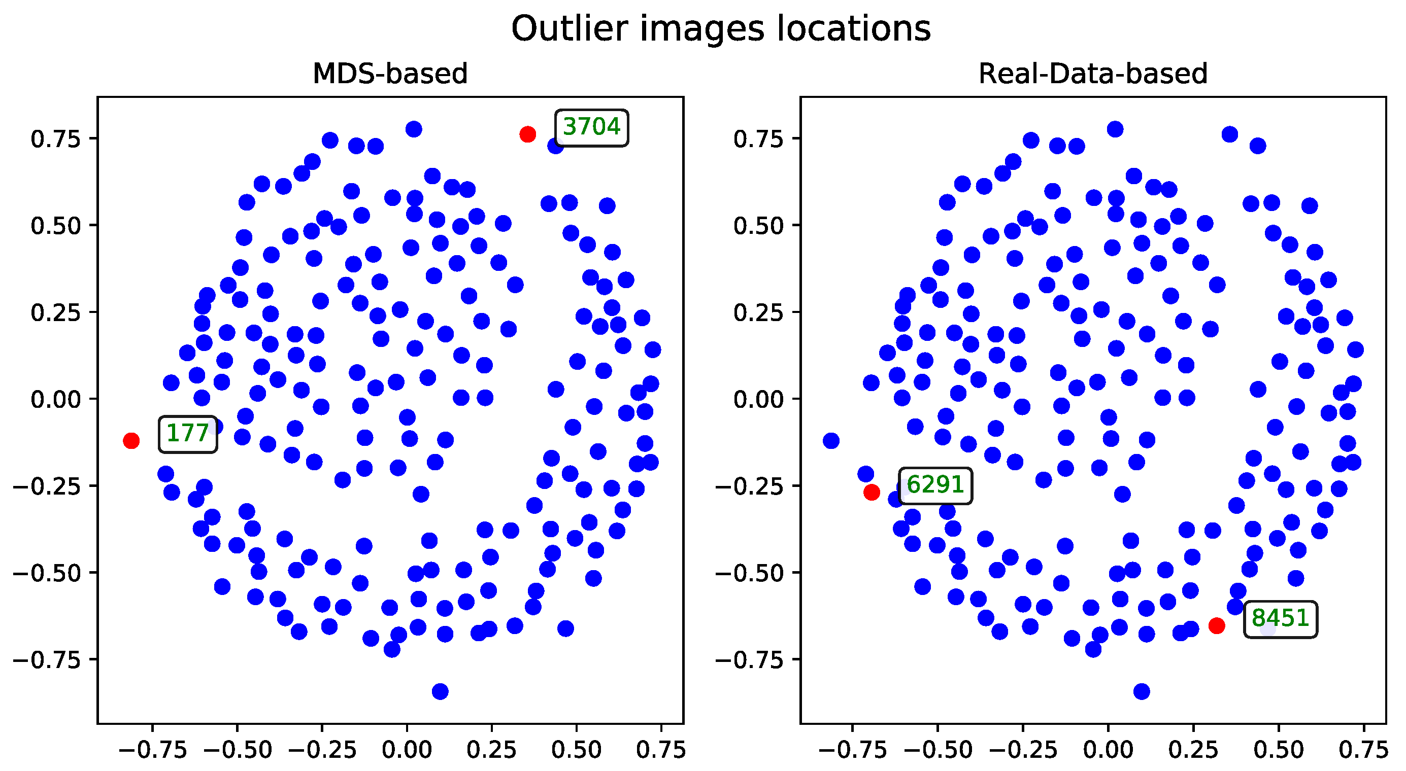
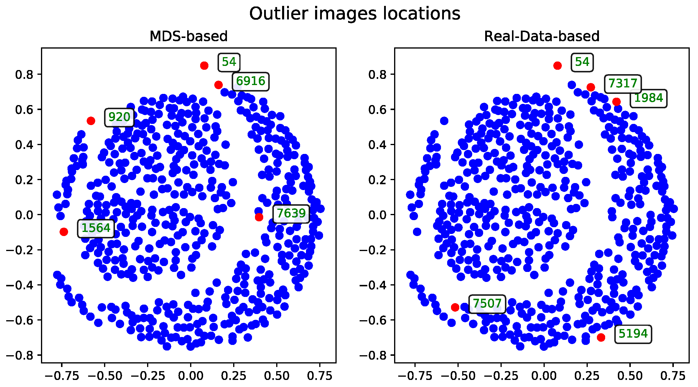
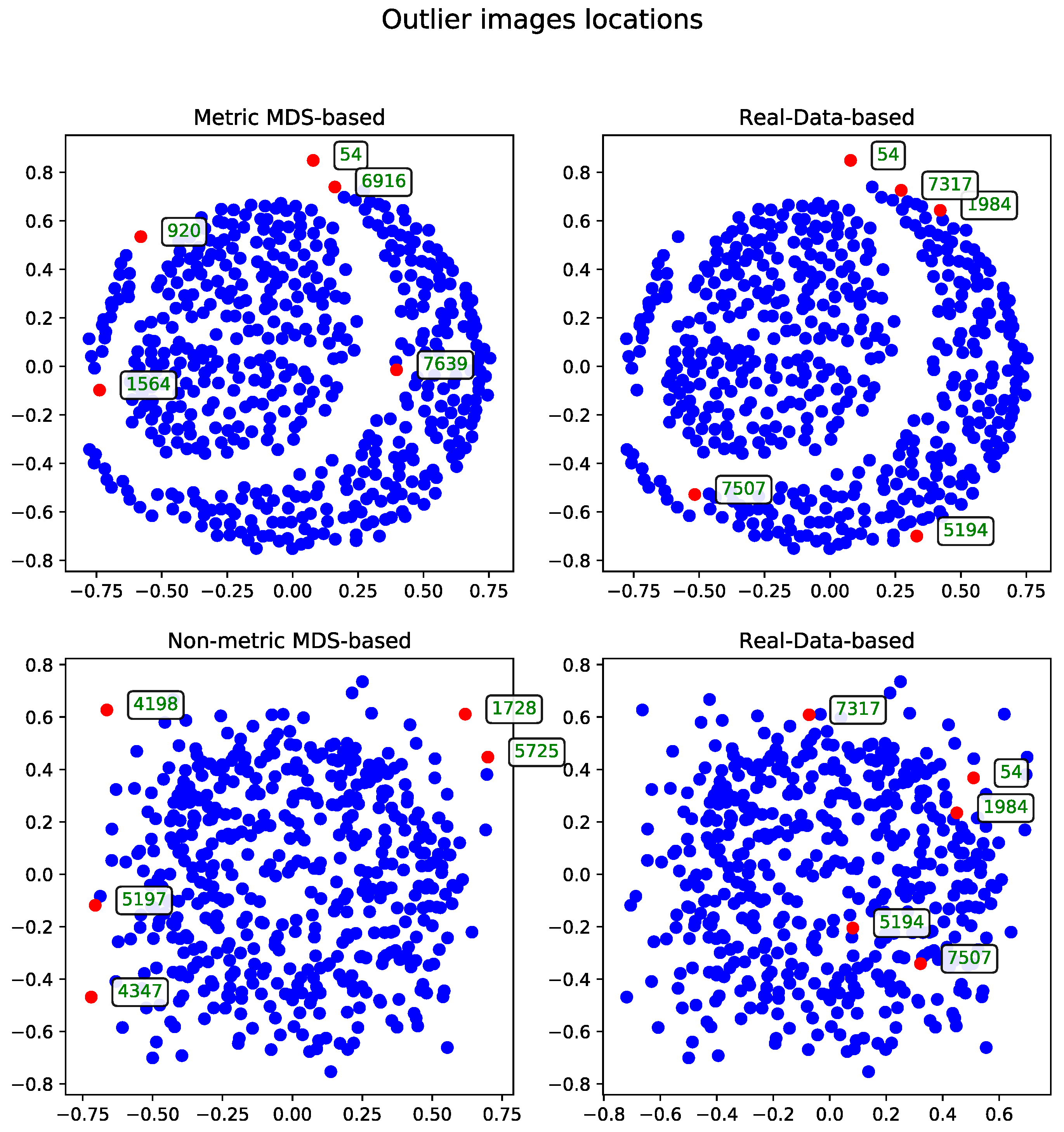
The MDS-based solution allows for intuitive visual detection of outliers in the reduced-dimensional space. Although the real-data-based method selects records based on their original distance profiles, these selections may not align perfectly with patterns observed after dimensionality reduction. However, some records—such as the one with ID 54—are consistently identified as outliers by both methods, underscoring their distinctiveness within the dataset.
Cosine Distance
The MDS algorithm was executed using the cosine distance matrix [
17]. The outliers identified by this method, alongside those detected using the real-data-based approach, are presented in
Figure 1.
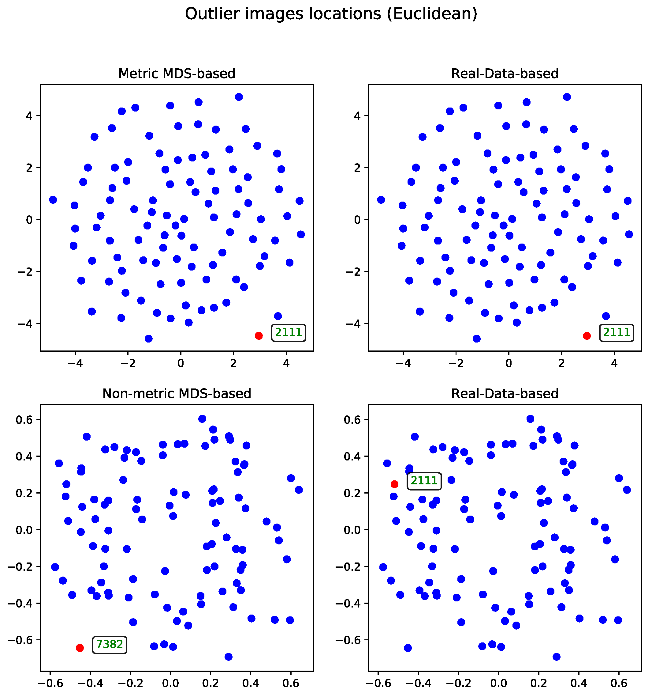
Metric Versus Non-Metric
The data can be processed using either the metric or non-metric version of the Multidimensional Scaling algorithm. The theoretical differences between the two are discussed in
Section 3.3, while the practical differences are illustrated in
Figure 2.
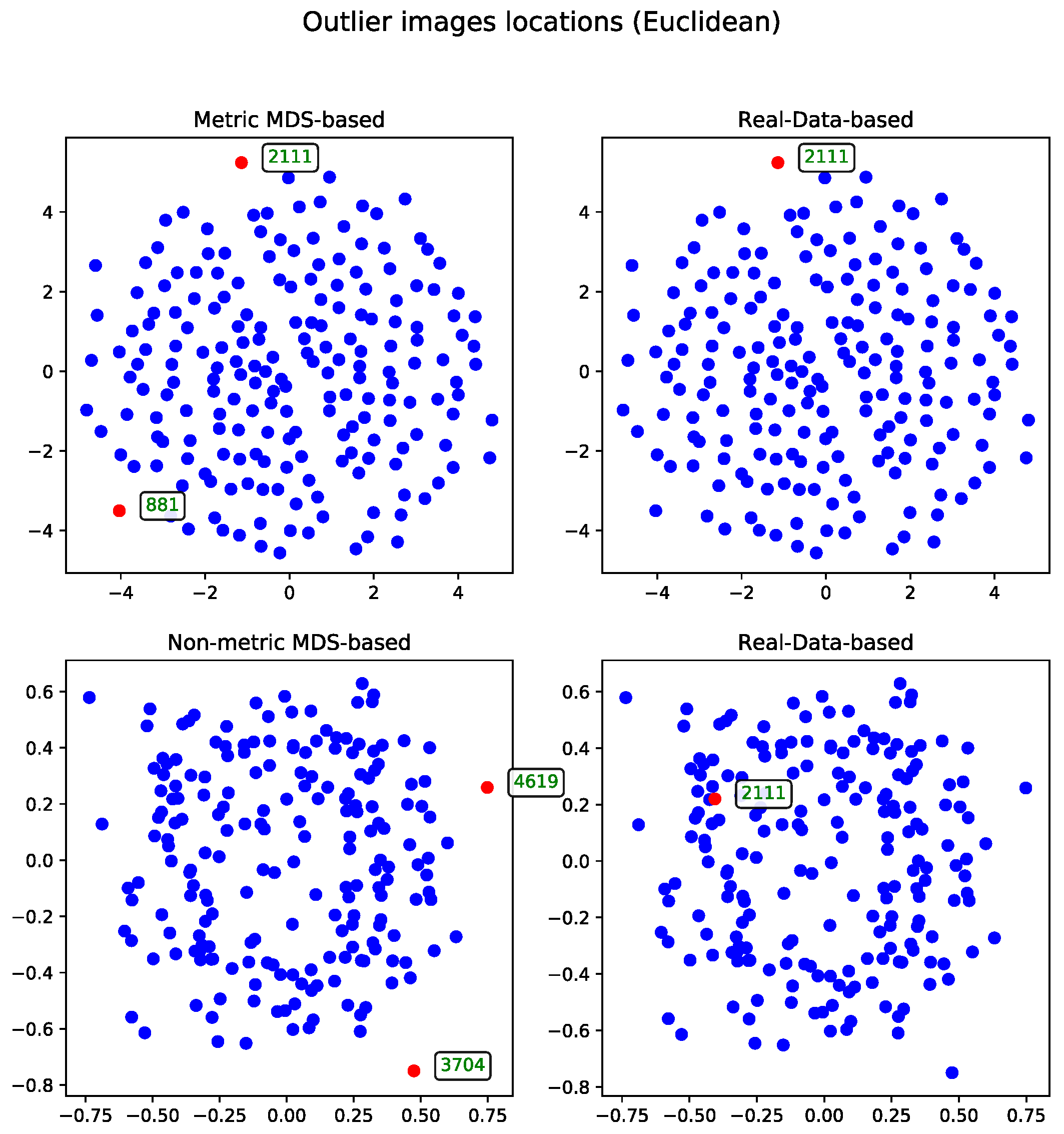
For comparison, the real-data-based solution is shown alongside both visualizations—one generated using metric MDS and the other using non-metric MDS. The non-metric MDS produces a less structured representation, often identifying outliers in a seemingly arbitrary manner. This behavior stems from its reliance on rank-based distance preservation rather than absolute distances. In contrast, the outliers detected by the real-data-based method show much stronger alignment with the metric MDS projection. Notably, all outliers selected by the real-data-based method are located within the lower crescent-shaped cluster, whereas the metric MDS highlights additional patterns and anomalies, offering a complementary perspective on the dataset.
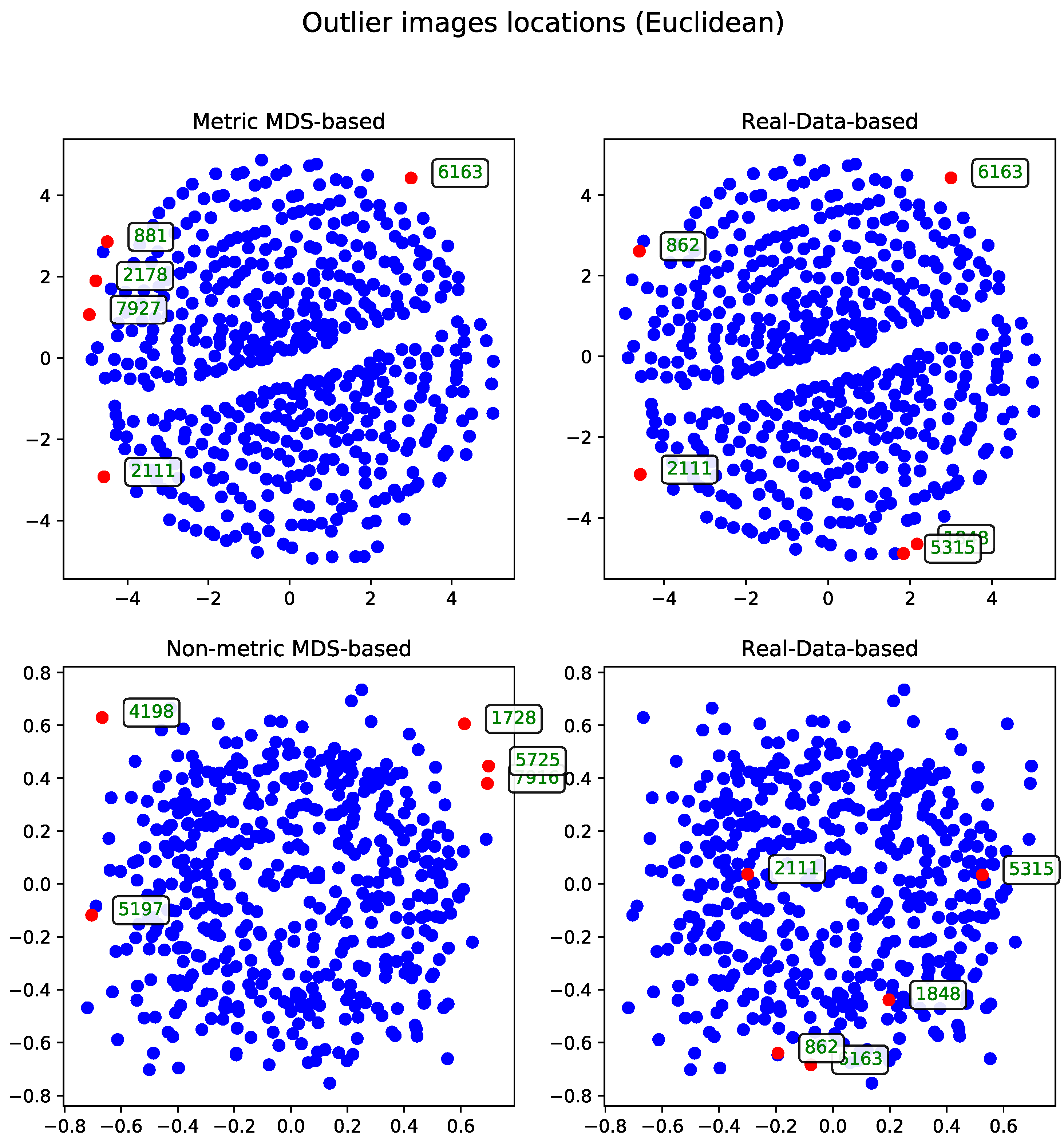
Euclidean Distance
The second approach to the MDS problem utilized the Euclidean distance matrix. Results from both the metric and non-metric MDS algorithms are presented for this configuration.
Figure 3 illustrates the outcomes of both methods—in a manner analogous to the comparison in Section Metric Versus Non-Metric.
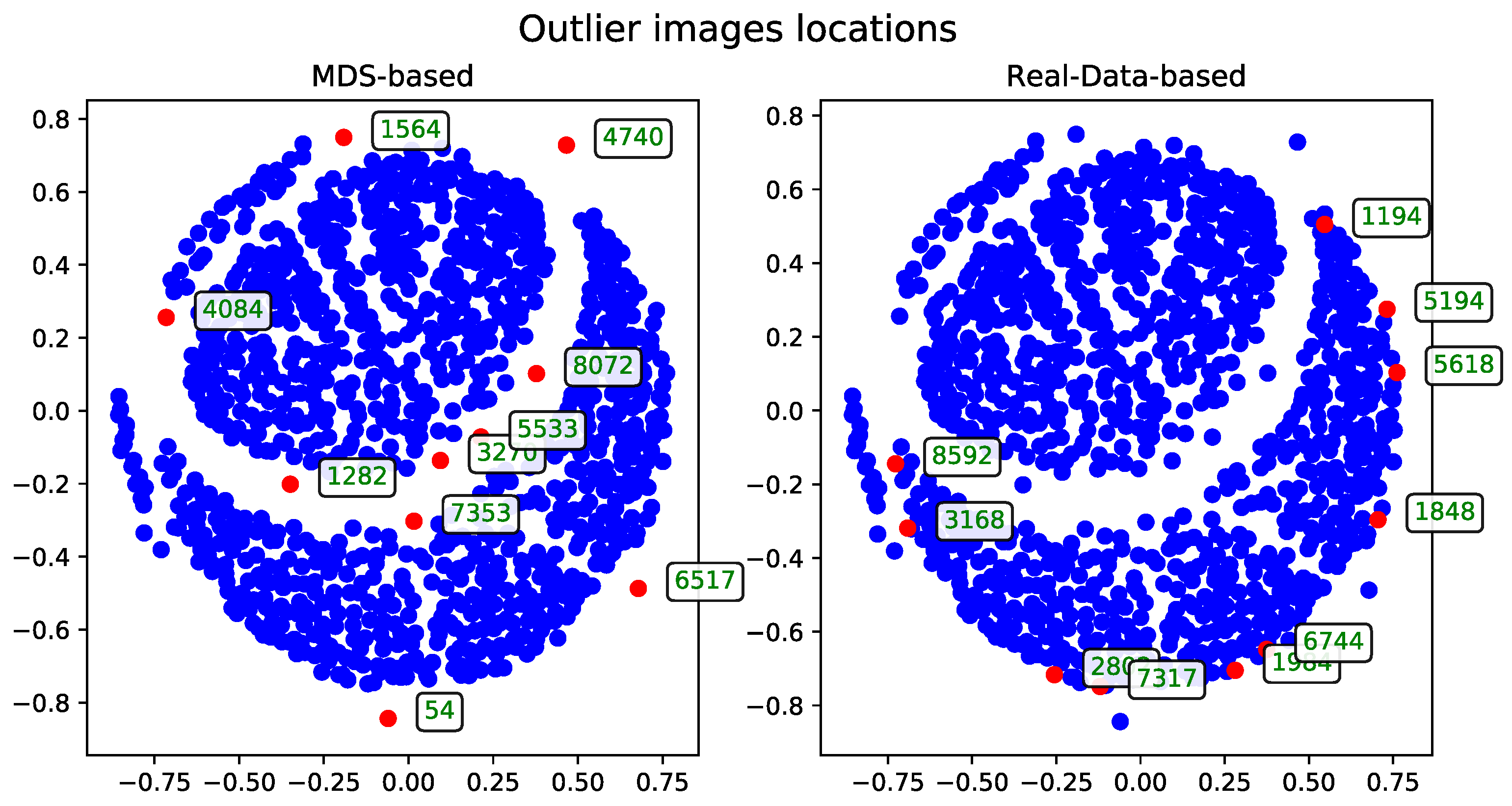
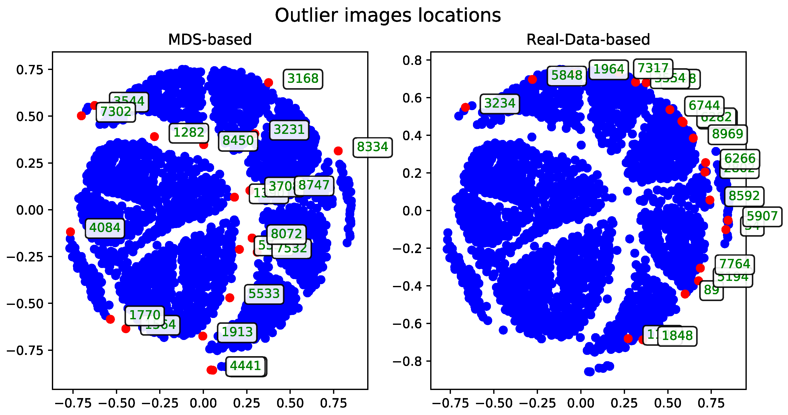
3.6.2. Agglomerative-Clustering-Based Solution–Agglomerative Outlier Selection
The dendrogram produced by the agglomerative clustering method serves as the foundation for identifying outlier records in the data. This approach can be applied using different affinity metrics and linkage algorithms.
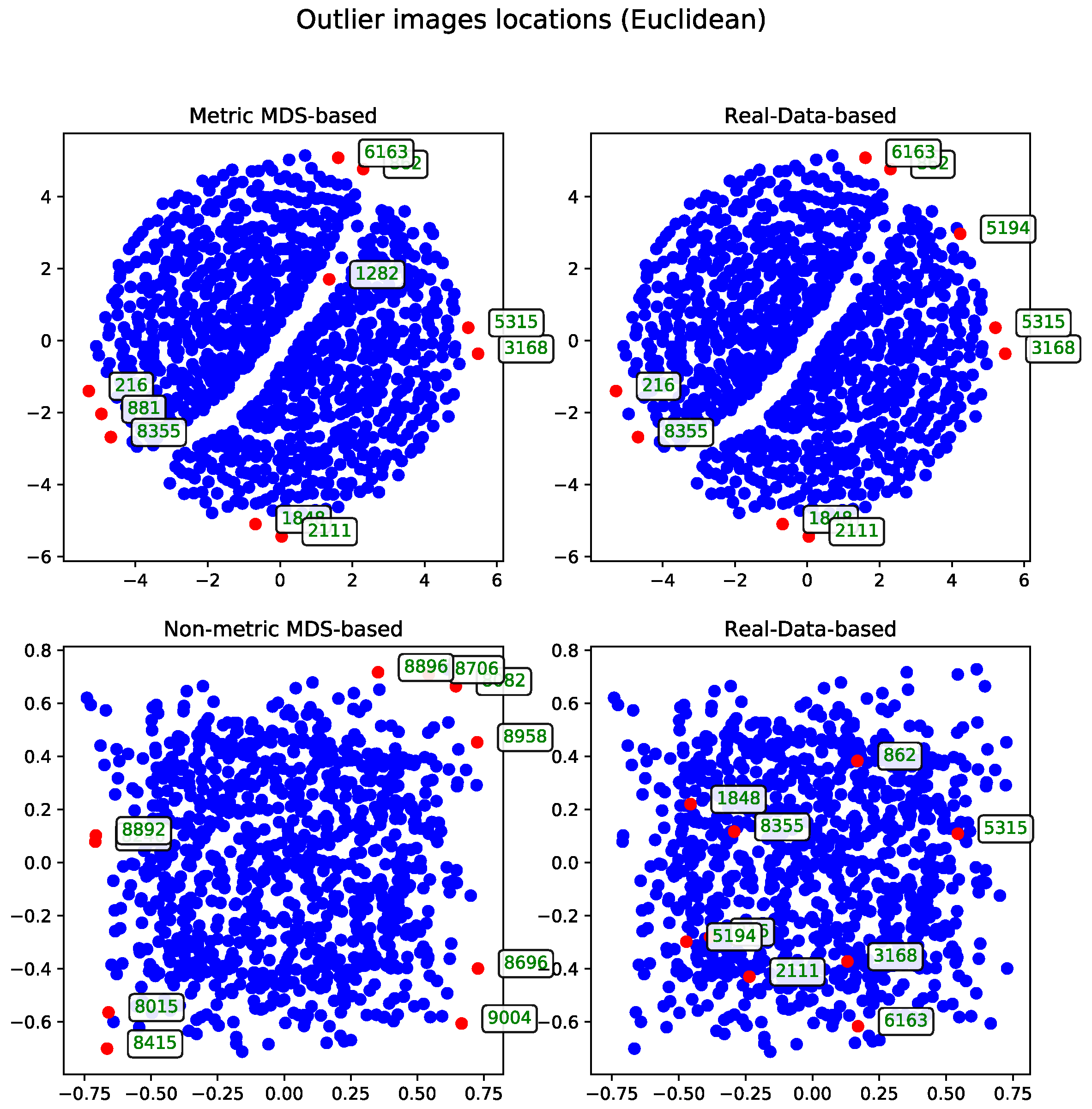
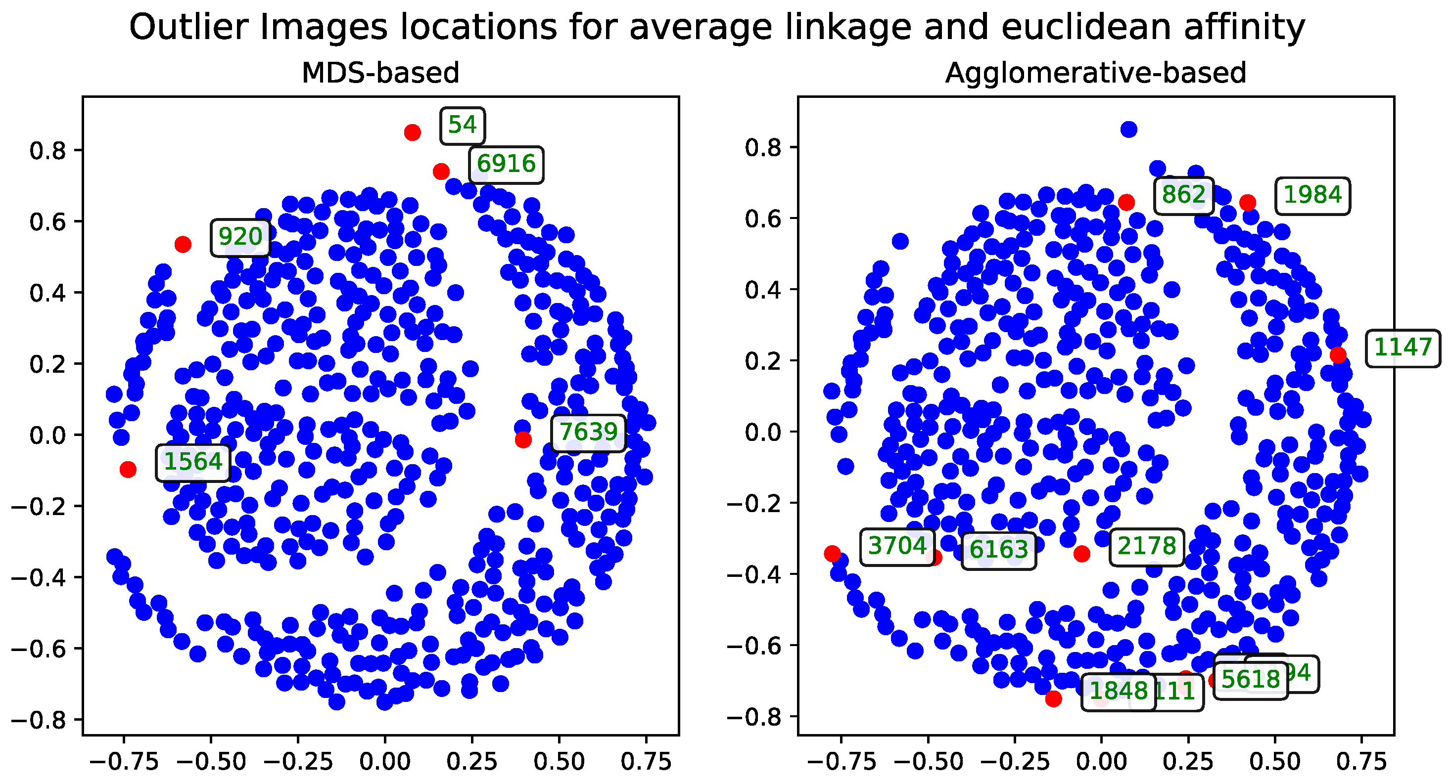
Euclidean Distance
The results calculated with Euclidean distance were produced using two dendrogram cutoff methods—level (
Figure 4) and last-
p (
Figure 5). Both methods are compared to the metric MDS approach based on the cosine distance matrix, which is also used to visualize the results.
The dendrogram cutoff parameters for both the level and last-
p methods were chosen to ensure that the number of detected outliers is comparable to those found by the MDS-based approaches, as detailed in
Section 3.5. This approach ensures the number of outliers is comparable across all methods.
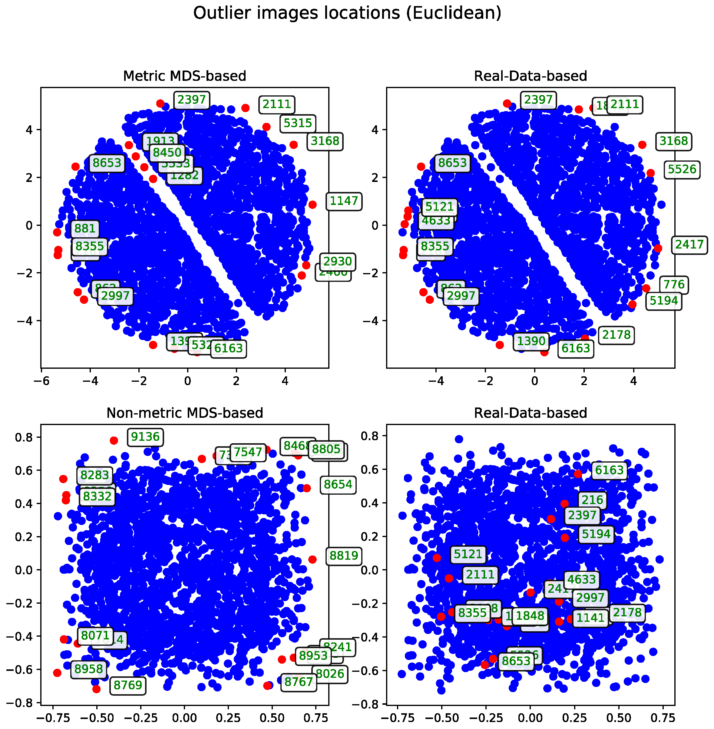
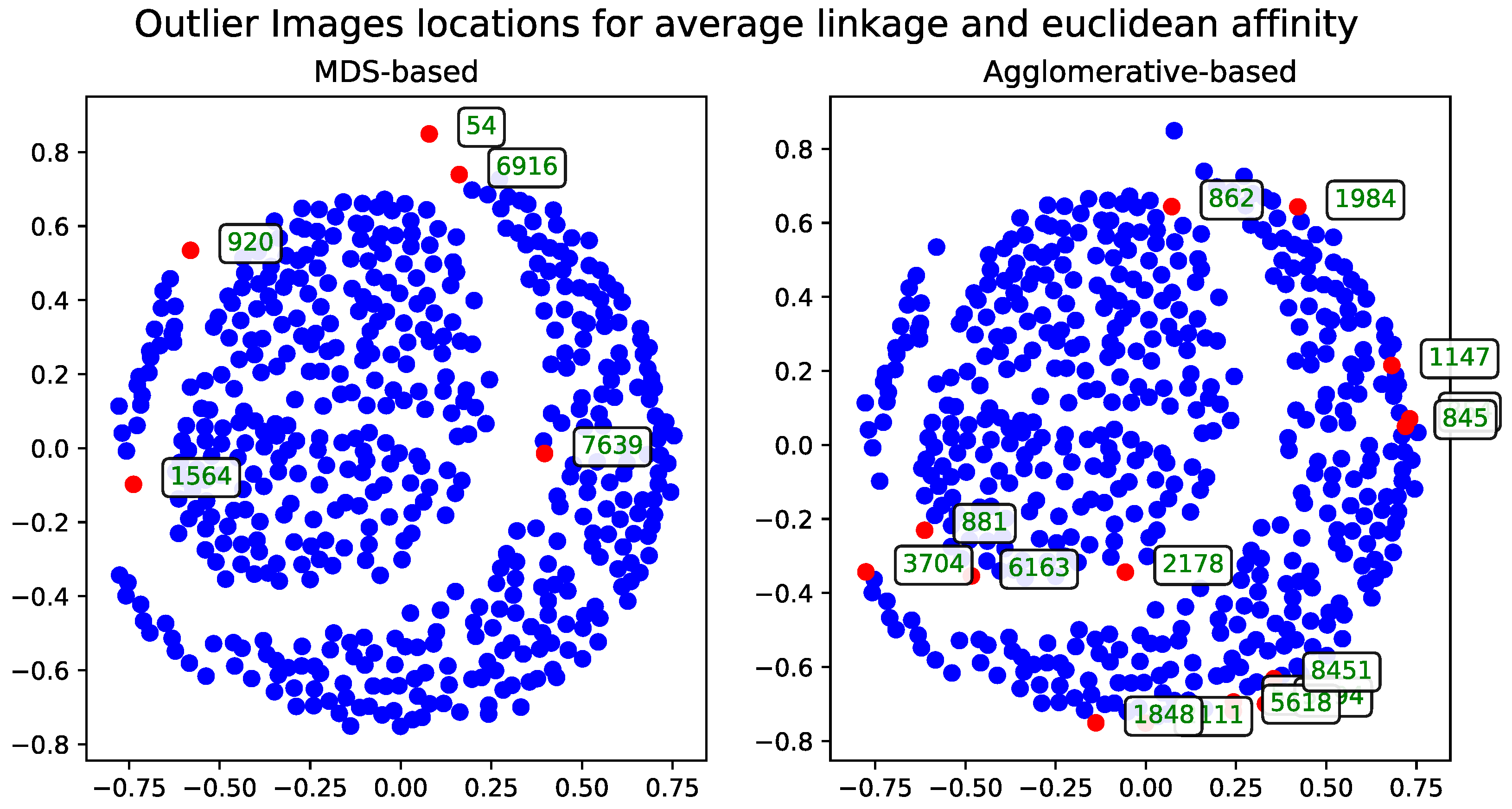
Cosine Distance
The agglomerative clustering dendrogram was also constructed using the cosine distance matrix. The AOS results obtained from this dendrogram were generated with two dendrogram cutoff methods—level (
Figure 6) and last-
p (
Figure 7). Both methods are compared to the metric MDS approach based on the cosine distance matrix, which is likewise used for visualizing the results.
The dendrogram cutoff parameters follow the selection criteria detailed in
Section 3.5.
4. Results and Practical Considerations
The outlier records identified by each method were gathered and are presented in the tables in this section. For practical reasons, all experiments that produced the results analyzed here were conducted only on the subset of 500 records. However, the methods can be safely applied to the other subsets as well. A selection of additional results obtained on other subset sizes is included in the
Appendix A, and supports the conclusions presented here. A summary of the outliers and their corresponding IDs, categorized by method and distance metric, is presented in
Table 2.
Table 2 and
Table 3 use consistent color coding and font styles to visually indicate outliers selected by multiple methods, allowing quick identification of overlaps across different algorithms and distance metrics.
Some records were identified as outliers by multiple methods, while others were flagged by only one. These overlaps are visually represented in
Table 2 using color and font style to highlight similarities between the selections. Not all methods returned the same number of outliers—particularly the AOS algorithm, whose output varied depending on the configuration. This variation is due to its dependence on the hierarchical structure of the dendrogram, where the number of selected records is influenced by the size and position of the clusters joined at the upper levels. Despite these differences, the total number of outliers selected by each method remains in the same order of magnitude, making the results comparable. The exact counts of outliers selected by each method and configuration are summarized in
Table 4.
As shown in
Table 4, the number of outliers selected by each method varies depending on both the algorithm and the chosen configuration. While the real-data-based method and both MDS variants consistently return five outliers—either by design or due to parameter selection—the AOS algorithm exhibits greater variability. This variability stems from its hierarchical nature, where the final selection is shaped by the dendrogram structure and the chosen cutoff strategy. The level-based cutoff typically selects fewer records than the last-
p variant, reflecting their differing assumptions about cluster granularity. These differences are further discussed in the context of parameter influence and selection strategies in
Section 3.5.
To further evaluate consistency among methods, each pair of algorithms was analyzed in terms of shared outlier selections. The analysis is summarized in two triangle-matrix-style tables.
Table 3 lists the specific record IDs that were selected as outliers by both methods in each pair. In contrast,
Table 5 presents the corresponding number of shared outliers per pair, offering a quantitative perspective on overlap.
Lastly, an outlier-oriented statistic was calculated for each method. This statistic served as the basis for constructing a metric for evaluating the outlier selection approaches. A higher value of the metric indicates that a greater number of outliers selected by a given method were also identified by other methods. The procedure for computing this evaluation metric is presented in Algorithm 3.
| Algorithm 3 ABEM: Agreement-Based Evaluation Metric for Outlier Selection Methods |
| 1: ▹ Number of methods |
| 2: ▹ Total number of unique outliers across all methods |
| 3: ▹ Binary presence matrix: outlier × method |
| 4: for to do |
| 5: for each outliers selected by method m do |
| 6: |
| 7: end for |
| 8: end for |
| 9: for to do ▹ Compute co-occurrence weights for each outlier |
| 10: |
| 11: end for |
| 12: for to do ▹ Compute average agreement score for each method |
| 13: |
| 14: end for |
| 15: Return sorted list of scores in descending order |
The Agreement-Based Evaluation Metric for Outlier Selection Methods (ABEM) captures the mean frequency with which the outliers selected by a given method also appear in the selections of other methods. As outlined in Algorithm 3, this is achieved by first constructing a binary matrix indicating which methods selected which outliers. The matrix is then weighted based on the number of methods that selected each outlier. Finally, for each method, the metric is computed as the average weight of its selected outliers. A higher value of this metric indicates stronger agreement between the evaluated method and the rest of the methods in the comparison set.
The results of applying the Agreement-Based Evaluation Metric for Outlier Selection Methods (ABEM) to the set of methods described in
Section 3—based on experiments conducted on the subset of 500 records—are presented in
Table 6. The table lists the mean ABEM values, providing a quantitative measure of how much each method’s selected outliers overlap with those selected by other methods. Higher values indicate greater agreement with the rest of the method set.
A value of ABEM close to 1 suggests that most outliers selected by the corresponding method were unique, i.e., not selected by any other method. This lack of overlap may indicate that the method captures a divergent notion of outliers, which could suggest lower practical reliability or efficiency. Conversely, higher ABEM values indicate greater agreement with other methods—meaning that outliers identified by the method were more frequently shared across the evaluation set. This consensus can be interpreted as a proxy for robustness, possibly pointing to a more effective or consistent approach to outlier detection.
To conclude, the Agreement-Based Evaluation Metric offers a compact and interpretable means of assessing consistency across outlier selection methods. Quantifying how frequently the selected outliers of each method are corroborated by others provides an additional perspective on their relative performance, complementing previous analyses and offering further support for practical method selection.
5. Concluding Remarks
This article presented an analysis of outlier record selection techniques using an incremental dataset of caption-described images, approached in a non-standard manner. While the captions were treated as the primary data, the corresponding images served merely as visual references, offering a human-readable interpretation of the described content. The captions were tokenized into individual words (tags), which were then used as the basis for analysis. In some methods, unsupervised preprocessing techniques such as MDS were employed to better structure the data.
Experiments were conducted on both the original and preprocessed versions of the dataset to identify potential outlier records. Images selected using the original data served as a reference for comparison. In addition to this baseline, three types of methods were employed for outlier detection: metric and non-metric MDS, and the proposed AOS method—an agglomerative clustering-based approach to outlier selection. All methods were evaluated using both Euclidean and cosine distance metrics. For AOS, an additional categorical hyperparameter was introduced to determine the dendrogram cutoff strategy.
In each case, outliers were successfully identified based on caption information. Using the proposed evaluation metric, the methods were assessed by the degree to which their selected outliers overlapped, i.e., how frequently individual records were identified by more than one method. The highest agreement was observed for the AOS method with level cutoff and Euclidean distance. However, the metric MDS-based method achieved the best performance under the cosine distance metric. Overall, the combination of all approaches provided the most comprehensive and robust outlier detection performance.
In the case of high-dimensional data, rather than identifying outliers directly in the original feature space, one can first apply preprocessing techniques that transform the data into more tractable representations. In this study, machine learning methods such as hierarchical clustering and dimensionality reduction via the MDS method were used as preprocessing steps for caption-based image descriptions. The experimental results confirm the effectiveness of these transformations in enhancing outlier selection quality.
The outlier selection methods introduced and evaluated here are generalizable and applicable across a wide range of datasets. Depending on the vector space used to construct the distance matrix, the methods may highlight different types of outliers—those that are distinct under varying distance perspectives. To fairly evaluate and compare the results of each method, an Agreement-Based Evaluation Metric was introduced. This non-parametric metric measures the average degree of consensus among methods by quantifying how frequently the same records are selected as outliers. The influence of input data preprocessing and vector representation on such consensus remains an open question for future work.


