
Scalar-on-Function Mode Estimation Using Entropy and Ergodic Properties of Functional Time Series Data

 , , ,
, , ,  and
and
Abstract
1. Introduction
1.1. Contributions of This Paper
1.2. Paper Organization
2. The -Recursive Estimation of the Mode
3. Main Results
- (Co1)
- (Co2)
- The function is three times continuously differentiable on . In addition, suppose that satisfies the Lipschitz conditionfor some , where is a neighborhood of .
- (Co3)
- The function is supported on and fulfills
- (Co4)
4. Discussion and Comments
4.1. On the Ergodic Functional Time Series
4.2. The Conditional Mode Versus the Conditional Mean
4.3. The Recursive Estimation in Action
4.4. The Computational Cost
5. Simulation Study
6. A Real Data Analysis
| Country | Sate | County | Code of Station | Geographical Coordinates |
| USA | lllinois | Champaign | BVL130 | 40.051981–88.372495 |
- Step 1. Randomly partition the dataset into two parts:
- –
- A training set, , consisting of 300 observations;
- –
- A test set, , consisting of 64 observations.
- Step 2. For each in the training set, predict the corresponding response by applying:
- –
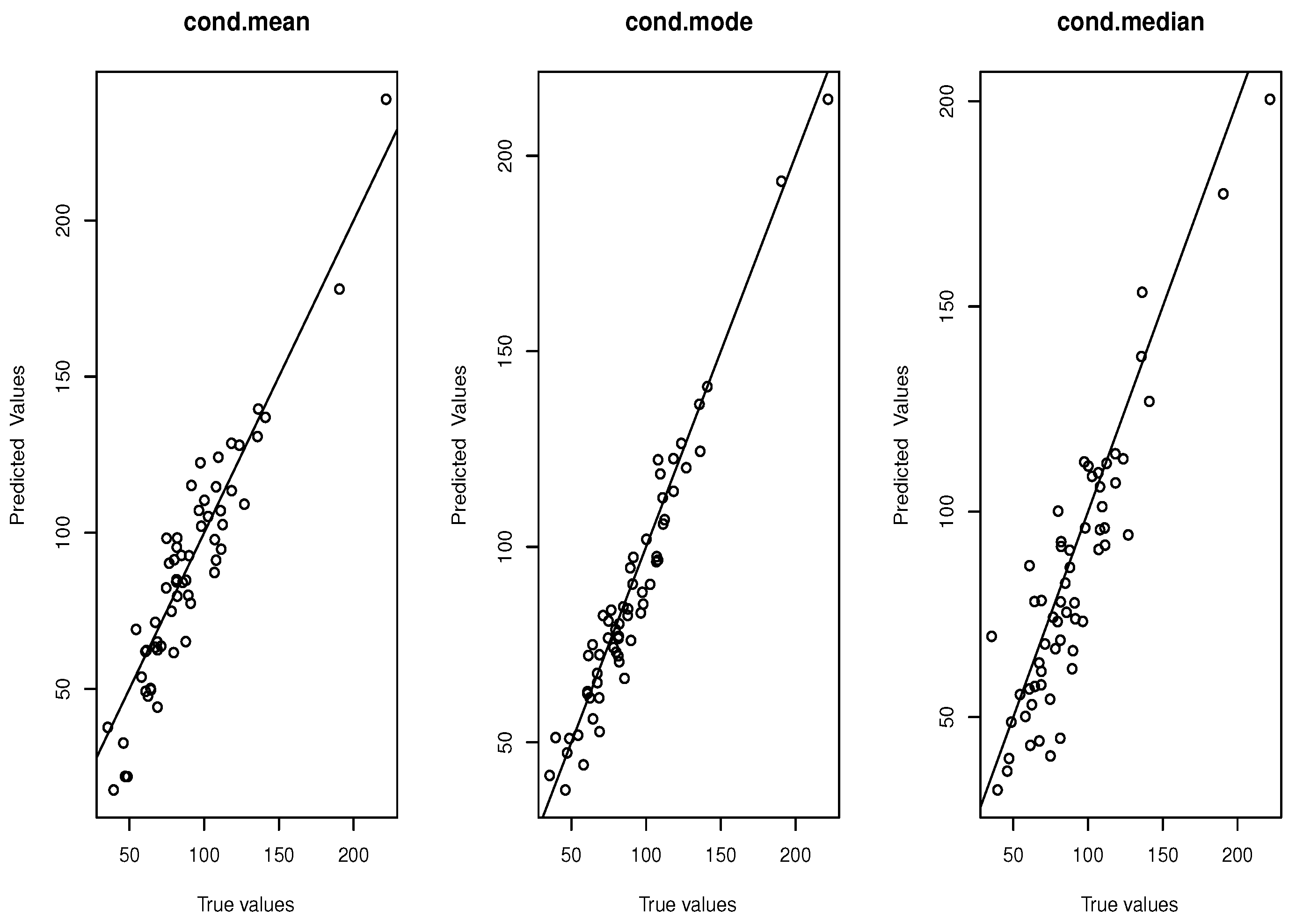
- Method 1 (Conditional mean):
- –
- Method 2 (Conditional mode):
- –
- Method 3 (Conditional median):
- Step 3. For each in the test set, identifywhere denotes the chosen distance function.
- Step 4. Use the identified index to predict :
- –
- Method 1 (Conditional mean):
- –
- Method 2 (Conditional mode):
- –
- Method 3 (Conditional median):
- Step 5. To assess the prediction accuracy among the methods, compute the square root of the mean squared error (SMSE):where can be , , or .
- Step 6. Plot the actual response values versus the predicted values for each method.
7. Conclusions
8. Proof of Propositions
Author Contributions
Funding
Data Availability Statement
Acknowledgments
Conflicts of Interest
References
- Collomb, G.; Härdle, W.; Hassani, S. A note on prediction via estimation of the conditional mode function. J. Stat. Plan. Inference 1986, 15, 227–236. [Google Scholar] [CrossRef]
- Quintela-Del-Rio, A.; Vieu, P. A nonparametric conditional mode estimate. J. Nonparametr. Stat. 1997, 8, 253–266. [Google Scholar] [CrossRef]
- Ioannides, D.; Matzner-Løber, E. A note on asymptotic normality of convergent estimates of the conditional mode with errors-in-variables. J. Nonparametr. Stat. 2004, 16, 515–524. [Google Scholar] [CrossRef]
- Louani, D.; Ould-Saïd, E. Asymptotic normality of kernel estimators of the conditional mode under strong mixing hypothesis. J. Nonparametr. Stat. 1999, 11, 413–442. [Google Scholar] [CrossRef]
- Allaoui, S.; Bouzebda, S.; Chesneau, C.; Liu, J. Uniform almost sure convergence and asymptotic distribution of the wavelet-based estimators of partial derivatives of multivariate density function under weak dependence. J. Nonparametr. Stat. 2021, 33, 170–196. [Google Scholar] [CrossRef]
- Ferraty, F.; Laksaci, A.; Vieu, P. Estimating some characteristics of the conditional distribution in nonparametric functional models. Stat. Inference Stoch. Process. 2006, 9, 47–76. [Google Scholar] [CrossRef]
- Dabo-Niang, S.; Kaid, Z.; Laksaci, A. On spatial conditional mode estimation for a functional regressor. Stat. Probab. Lett. 2012, 82, 1413–1421. [Google Scholar] [CrossRef]
- Ezzahrioui, M.H.; Ould-Saïd, E. Asymptotic normality of a nonparametric estimator of the conditional mode function for functional data. J. Nonparametr. Stat. 2008, 20, 3–18. [Google Scholar] [CrossRef]
- Ezzahrioui, M.H.; Saïd, E.O. Some asymptotic results of a non-parametric conditional mode estimator for functional time-series data. Stat. Neerl. 2010, 64, 171–201. [Google Scholar] [CrossRef]
- Ferraty, F.; Vieu, P. Functional Nonparametric Prediction Methodologies. In Nonparametric Functional Data Analysis: Theory and Practice; Springer: New York, NY, USA, 2006; pp. 49–59. [Google Scholar]
- Dabo-Niang, S.; Kaid, Z.; Laksaci, A. Asymptotic properties of the kernel estimate of spatial conditional mode when the regressor is functional. AStA Adv. Stat. Anal. 2015, 99, 131–160. [Google Scholar] [CrossRef]
- Bouanani, O.; Laksaci, A.; Rachdi, M.; Rahmani, S. Asymptotic normality of some conditional nonparametric functional parameters in high-dimensional statistics. Behaviormetrika 2019, 46, 199–233. [Google Scholar] [CrossRef]
- Ling, N.; Liu, Y.; Vieu, P. Conditional mode estimation for functional stationary ergodic data with responses missing at random. Statistics 2016, 50, 991–1013. [Google Scholar] [CrossRef]
- Almanjahie, I.M.; Kaid, Z.; Laksaci, A.; Rachdi, M. Estimating the conditional density in scalar-on-function regression structure: K-NN local linear approach. Mathematics 2022, 10, 902. [Google Scholar] [CrossRef]
- Attouch, M.; Bouabsa, W. The k-nearest neighbors estimation of the conditional mode for functional data. Rev. Roum. Math. Pures Appl. 2013, 58, 393–415. [Google Scholar]
- Azzi, A.; Belguerna, A.; Laksaci, A.; Rachdi, M. The scalar-on-function modal regression for functional time series data. J. Nonparametr. Stat. 2024, 36, 503–526. [Google Scholar] [CrossRef]
- Wang, T. Non-parametric Estimator for Conditional Mode with Parametric Features. Oxf. Bull. Econ. Stat. 2024, 86, 44–73. [Google Scholar] [CrossRef]
- Schouten, B.; Klausch, T.; Buelens, B.; Van Den Brakel, J. A Cost–Benefit Analysis of Reinterview Designs for Estimating and Adjusting Mode Measurement Effects: A Case Study for the Dutch Health Survey and Labour Force Survey. J. Surv. Stat. Methodol. 2024, 12, 790–813. [Google Scholar] [CrossRef]
- Guenani, S.; Bouabsa, W.; Omar, F.; Kadi Attouch, M.; Khardani, S. Some asymptotic results of a kNN conditional mode estimator for functional stationary ergodic data. Commun. Stat.-Theory Methods 2024, 54, 3094–3113. [Google Scholar] [CrossRef]
- Thiam, A.; Thiam, B.; Crambes, C. Recursive estimation of nonparametric regression with functional covariate. Qual. Control Appl. Stat. 2014, 59, 527–528. [Google Scholar]
- Slaoui, Y. Recursive nonparametric regression estimation for dependent strong mixing functional data. Stat. Inference Stoch. Process. 2020, 23, 665–697. [Google Scholar] [CrossRef]
- Alamari, M.B.; Almulhim, F.A.; Litimein, O.; Mechab, B. Strong Consistency of Incomplete Functional Percentile Regression. Axioms 2024, 13, 444. [Google Scholar] [CrossRef]
- Shang, H.L.; Yang, Y. Nonstationary functional time series forecasting. J. Forecast. 2024. early view. [Google Scholar] [CrossRef]
- Aneiros, G.; Horová, I.; Hušková, M.; Vieu, P. Special Issue on Functional Data Analysis and Related Fields. J. Multivar. Anal. 2022, 189, 104908. [Google Scholar] [CrossRef]
- Moindjié, I.A.; Preda, C.; Dabo-Niang, S. Fusion regression methods with repeated functional data. Comput. Stat. Data Anal. 2025, 203, 108069. [Google Scholar] [CrossRef]
- Gertheiss, J.; Rügamer, D.; Liew, B.X.; Greven, S. Functional data analysis: An introduction and recent developments. Biom. J. 2024, 66, e202300363. [Google Scholar] [CrossRef]
- Agua, B.M.; Bouzebda, S. Single index regression for locally stationary functional time series. AIMS Math. 2024, 9, 36202–36258. [Google Scholar] [CrossRef]
- Bouanani, O.; Bouzebda, S. Limit theorems for local polynomial estimation of regression for functional dependent data. AIMS Math. 2024, 9, 23651–23691. [Google Scholar] [CrossRef]
- Bouzebda, S. Weak convergence of the conditional single index U-statistics for locally stationary functional time series. AIMS Math. 2024, 9, 14807–14898. [Google Scholar] [CrossRef]
- Xu, R.; Wang, J. L 1-estimation for spatial nonparametric regression. J. Nonparametr. Stat. 2008, 20, 523–537. [Google Scholar] [CrossRef]
- Andrews, D. First Order Autoregressive Processes and Strong Mixing; Cowles Foundation Discussion Papers 664. Cowles Foundation for Research in Economics; Yale University: New Haven, CT, USA, 1983. [Google Scholar]
- Beran, J. Statistics for Long-Memory Processes; Routledge: London, UK, 2017. [Google Scholar]
- Ibragimov, I.A.; Rozanov, Y.A.E. Gaussian Random Processes; Springer Science & Business Media: Berlin/Heidelberg, Germany, 2012; Volume 9. [Google Scholar]
- Magdziarz, M.; Weron, A. Ergodic properties of anomalous diffusion processes. Ann. Phys. 2011, 326, 2431–2443. [Google Scholar] [CrossRef]
- Aneiros-Pérez, G.; Cardot, H.; Estévez-Pérez, G.; Vieu, P. Maximum ozone concentration forecasting by functional non-parametric approaches. Environmetrics 2004, 15, 675–685. [Google Scholar] [CrossRef]


| MF | FTS | Dist. | Het. | Hom. | SNRHet (5%) | SNRHet (40%) |
|---|---|---|---|---|---|---|
| MF = 1 | GFAR(2) | Laplace | 0.176 | 0.154 | 1.174 | 2.197 |
| Log normal | 0.183 | 0.166 | 1.187 | 2.198 | ||
| Weibull | 0.196 | 0.172 | 1.189 | 2.208 | ||
| WFAR(2) | Laplace | 0.165 | 0.143 | 0.158 | 2.171 | |
| Log normal | 0.173 | 0.141 | 1.153 | 2.185 | ||
| Weibull | 0.170 | 0.153 | 1.170 | 2.192 | ||
| FARCH(1) | Laplace | 0.201 | 0.182 | 1.204 | 2.209 | |
| Log normal | 0.223 | 0.209 | 1.311 | 2.534 | ||
| Weibull | 0.240 | 0.223 | 1.412 | 2.626 | ||
| MF = 10 | GFAR(2) | Laplace | 0.256 | 0.261 | 1.353 | 2.413 |
| Log normal | 0.317 | 0.312 | 1.487 | 2.507 | ||
| Weibull | 0.296 | 0.542 | 1.618 | 2.698 | ||
| WFAR(2) | Laplace | 0.356 | 0.334 | 1.385 | 0.497 | |
| Log normal | 0.432 | 0.513 | 1.635 | 2.758 | ||
| Weibull | 0.408 | 0.443 | 1.489 | 2.595 | ||
| FARCH(1) | Laplace | 0.513 | 0.523 | 1.641 | 2.691 | |
| Log normal | 0.434 | 0.419 | 1.453 | 2.554 | ||
| Weibull | 0.504 | 0.514 | 1.562 | 1.516 |
| MF | FTS | Dist. | HeT. | Hom. | SNRHet (5%) | SNRHet (40%) |
|---|---|---|---|---|---|---|
| MF = 1 | GFAR(2) | Laplace | 1.161 | 1.109 | 2.008 | 4.378 |
| Log normal | 1.304 | 0.963 | 2.789 | 4.678 | ||
| Weibull | 3.239 | 2.107 | 3.896 | 4.894 | ||
| WFAR(2) | Laplace | 0.876 | 0.403 | 1.097 | 1.856 | |
| Log normal | 0.606 | 0.236 | 1.765 | 2.785 | ||
| Weibull | 1.690 | 1.327 | 2.045 | 2.976 | ||
| FARCH(1) | Laplace | 2.332 | 1.763 | 2.435 | 4.554 | |
| Log normal | 2.204 | 1.398 | 3.971 | 5.861 | ||
| Weibull | 5.109 | 3.712 | 5.023 | 6.432 | ||
| MF = 10 | GFAR(2) | Laplace | 4.201 | 4.216 | 7.312 | 8.417 |
| Log normal | 4.230 | 4.736 | 6.789 | 7.678 | ||
| Weibull | 5.117 | 6.107 | 7.186 | 8.243 | ||
| WFAR(2) | Laplace | 3.654 | 3.212 | 4.178 | 5.164 | |
| Log normal | 3.902 | 4.561 | 5.605 | 6.194 | ||
| Weibull | 4.310 | 4.127 | 6.205 | 6.817 | ||
| FARCH(1) | Laplace | 6.231 | 7.862 | 8.333 | 9.352 | |
| Log normal | 4.315 | 5.493 | 6.771 | 8.662 | ||
| Weibull | 7.101 | 7.513 | 8.224 | 9.533 |
| MF | FTS | Dist. | Het. | Hom. | SNRHet (5%) | SNRHet (40%) |
|---|---|---|---|---|---|---|
| MF = 1 | GFAR(2) | Laplace | 1.535 | 1.331 | 2.103 | 4.414 |
| Log normal | 1.202 | 1.106 | 2.452 | 4.786 | ||
| Weibull | 2.119 | 1.811 | 3.02 | 4.949 | ||
| WFAR(2) | Laplace | 0.167 | 0.156 | 1.861 | 3.843 | |
| Log normal | 0.134 | 0.136 | 1.451 | 3.073 | ||
| Weibull | 0.109 | 0.117 | 0.698 | 1.785 | ||
| FARCH(1) | Laplace | 3.101 | 2.512 | 3.972 | 4.952 | |
| Log normal | 2.603 | 2.363 | 3.861 | 5.045 | ||
| Weibull | 4.009 | 3.227 | 4.961 | 5.895 | ||
| MF = 10 | GFAR(2) | Laplace | 2.552 | 2.312 | 4.132 | 6.447 |
| Log normal | 2.221 | 3.166 | 5.421 | 8.761 | ||
| Weibull | 4.191 | 5.823 | 6.211 | 8.991 | ||
| WFAR(2) | Laplace | 2.171 | 2.164 | 4.812 | 6.832 | |
| Log normal | 2.142 | 0.162 | 1.412 | 3.264 | ||
| Weibull | 2.192 | 2.173 | 3.682 | 5.751 | ||
| FARCH(1) | Laplace | 8.112 | 8.521 | 9.128 | 9.921 | |
| Log normal | 4.611 | 4.169 | 6.161 | 10.012 | ||
| Weibull | 9.018 | 10.271 | 11.031 | 12.185 |
| Model | Metric | Kernel | SMSE |
|---|---|---|---|
| PCA (3th eigenfunction) | Quadratic kernel | 3.26 | |
| PCA (3th eigenfunction) | -kernel | 3.37 | |
| 8th eigenfunction | Quadratic kernel | 4.03 | |
| 8th eigenfunction | -kernel | 4.11 | |
| Spline metric | Quadratic kernel | 4.39 | |
| Spline metric | -kernel | 4.52 | |
| PCA (3th eigenfunction) | Quadratic kernel | 5.42 | |
| PCA (3th eigenfunction) | -kernel | 5.61 | |
| 8th eigenfunction | Quadratic kernel | 7.56 | |
| 8th eigenfunction | -kernel | 8.22 | |
| Spline metric | Quadratic kernel | 6.45 | |
| Spline metric | -kernel | 6.82 | |
| PCA (3th eigenfunction) | Quadratic kernel | 4.87 | |
| PCA (3th eigenfunction) | -kernel | 5.11 | |
| 8th eigenfunction | Quadratic kernel | 8.62 | |
| 8th eigenfunction | -kernel | 8.34 | |
| Spline metric | Quadratic kernel | 6.12 | |
| Spline metric | -kernel | 6.73 |
Disclaimer/Publisher’s Note: The statements, opinions and data contained in all publications are solely those of the individual author(s) and contributor(s) and not of MDPI and/or the editor(s). MDPI and/or the editor(s) disclaim responsibility for any injury to people or property resulting from any ideas, methods, instructions or products referred to in the content. |
© 2025 by the authors. Licensee MDPI, Basel, Switzerland. This article is an open access article distributed under the terms and conditions of the Creative Commons Attribution (CC BY) license (https://creativecommons.org/licenses/by/4.0/).
Share and Cite
Alamari, M.B.; Almulhim, F.A.; Almanjahie, I.M.; Bouzebda, S.; Laksaci, A. Scalar-on-Function Mode Estimation Using Entropy and Ergodic Properties of Functional Time Series Data. Entropy 2025, 27, 552. https://doi.org/10.3390/e27060552
Alamari MB, Almulhim FA, Almanjahie IM, Bouzebda S, Laksaci A. Scalar-on-Function Mode Estimation Using Entropy and Ergodic Properties of Functional Time Series Data. Entropy. 2025; 27(6):552. https://doi.org/10.3390/e27060552
Chicago/Turabian StyleAlamari, Mohammed B., Fatimah A. Almulhim, Ibrahim M. Almanjahie, Salim Bouzebda, and Ali Laksaci. 2025. "Scalar-on-Function Mode Estimation Using Entropy and Ergodic Properties of Functional Time Series Data" Entropy 27, no. 6: 552. https://doi.org/10.3390/e27060552
APA StyleAlamari, M. B., Almulhim, F. A., Almanjahie, I. M., Bouzebda, S., & Laksaci, A. (2025). Scalar-on-Function Mode Estimation Using Entropy and Ergodic Properties of Functional Time Series Data. Entropy, 27(6), 552. https://doi.org/10.3390/e27060552