
Baselining Urban Ecosystems from Sentinel Species: Fitness, Flows, and Sinks


Abstract

1. Introduction
1.1. Computational Eco-Complexity Approach to Ecosystem Fitness
1.2. Species as Indicators of Ecosystem Fitness Stressed by the Climate: Inferring Magnitude and Pathways of Change
1.3. A Structural Ecological Framework for Ecosystem Assessment and Design: The Ecosystem Fitness Index
2. Materials and Methods: Digital Ecosystem Models
2.1. Data
2.2. MaxEnt and Multiplex Habitat Suitability Landscape
2.3. Digital Ecosystem Models: Inference of Ecological Flows and Attraction Basins
2.4. Ecosystem Fitness Index
3. Results
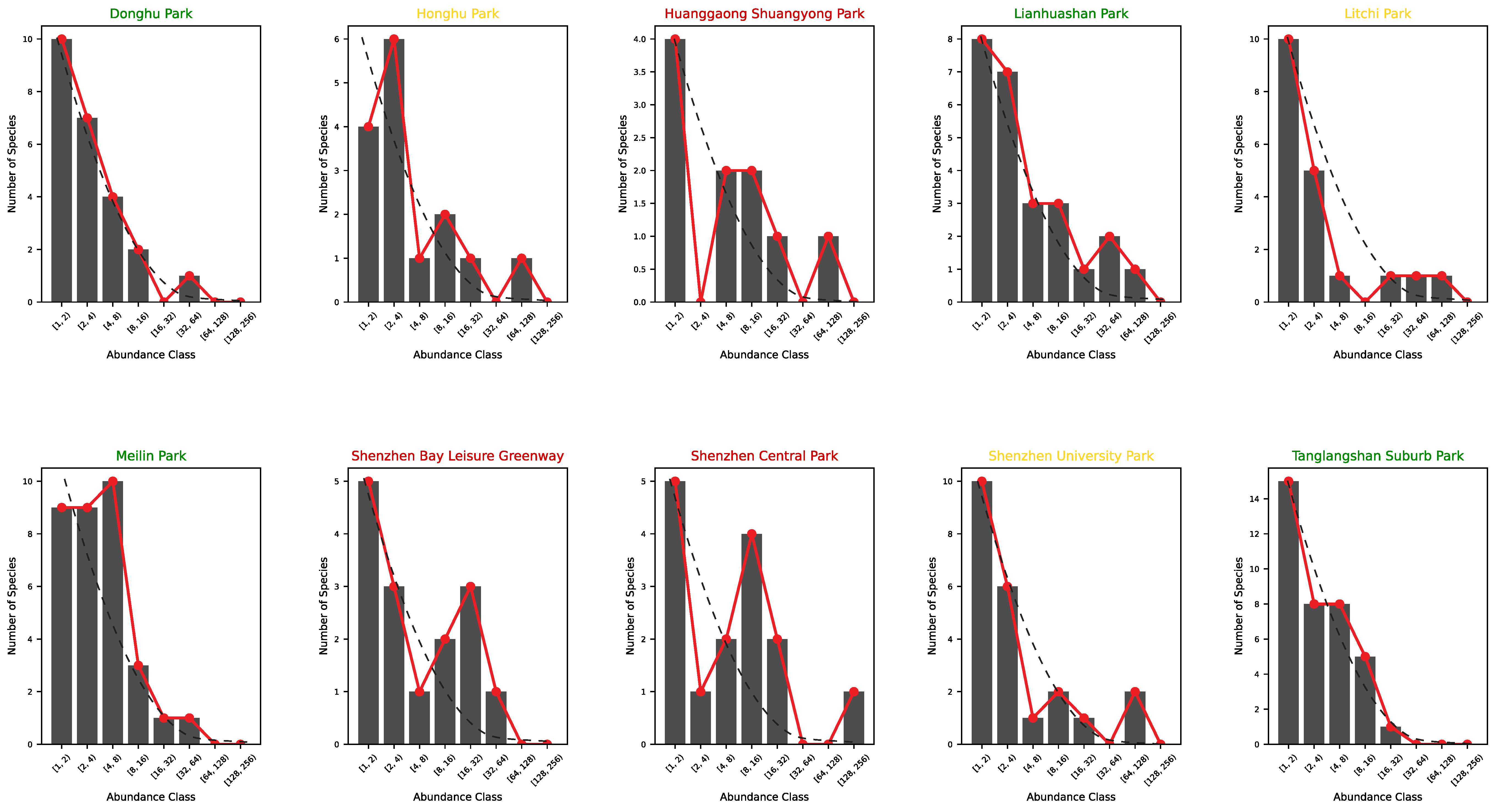
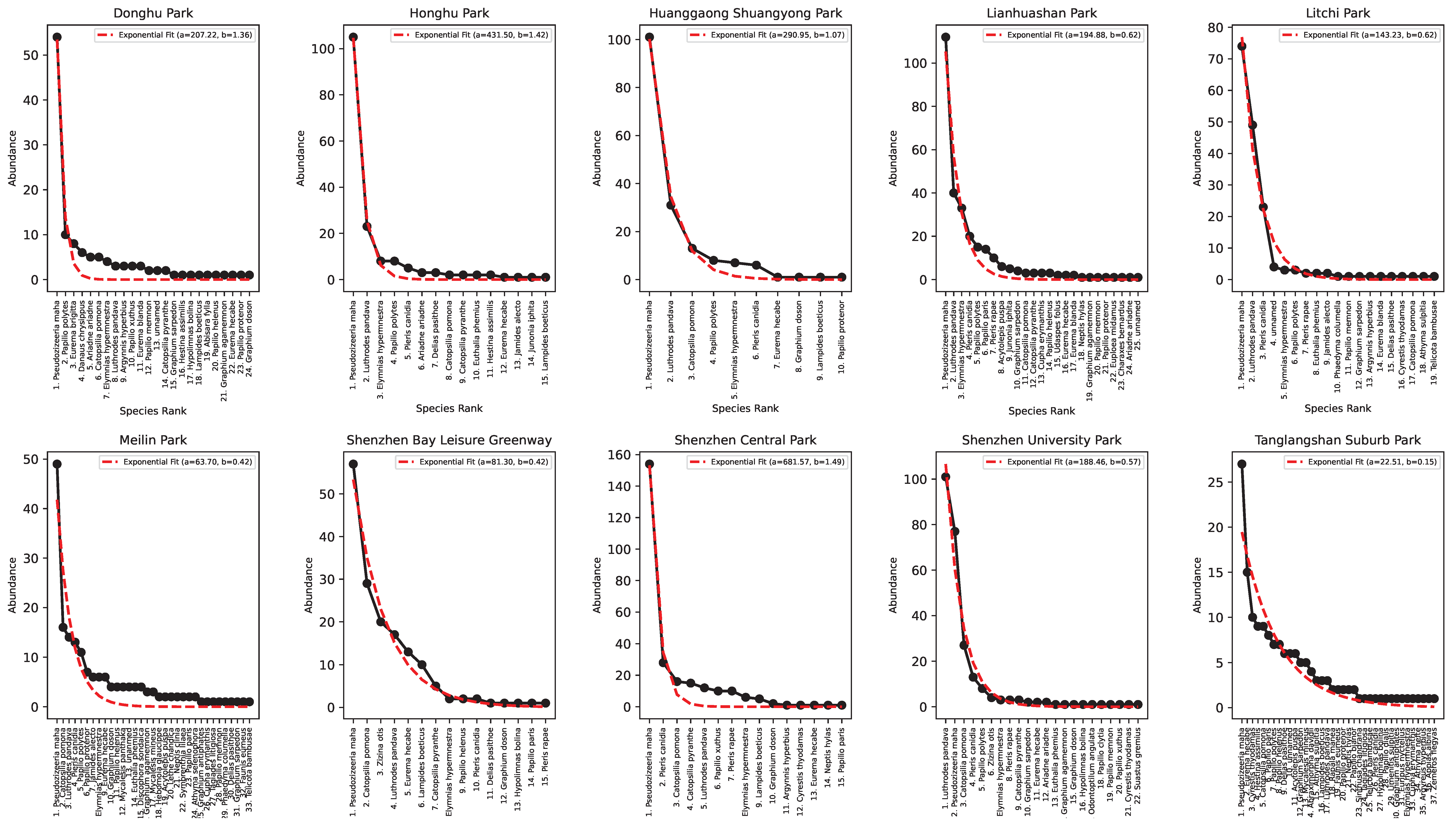
- (A) Tanglangshan, Meilin, Donghu, and Linahuashan are healthy parks with the highest joint fitness (as HS and convergence to the log-normal Preston plot). These parks also have a relatively high interconnectedness with each other and are not directly proximal to areas with high residential density. However, they have a high FLII (as in Grantham et al. [39] available at https://www.forestintegrity.com/ (accessed on 16 April 2025)) or are proximal to forests with high FLIIs and hydrogeomorphic heterogeneity (Tanglangshan has the only forest overlapping with the whole park in West–Central Shenzhen). These high-EFI sites are ecotones between natural areas and densely populated areas.
- (B) Lithchi, SZ University, and Honghu have intermediate fitness due to the higher percentage of high-abundance classes that make the Preston plot better, even across species. These parks are much smaller and closer to areas with high residential density.
- (C) Huanggaong, SZ Central, and SZ Bay leisure greenway have a low EFI because of their bimodal Preston plots, indicating two bistable states in species–abundance. This bistability may suggest some instability compared to other parks. These parks are smaller and closer to high-residential-density areas. These areas are much further from high-FLII areas and have very low hydrogeomorphic variability.
4. Discussion
4.1. Modeling Innovations: Inference of the Functional Ecological Architecture
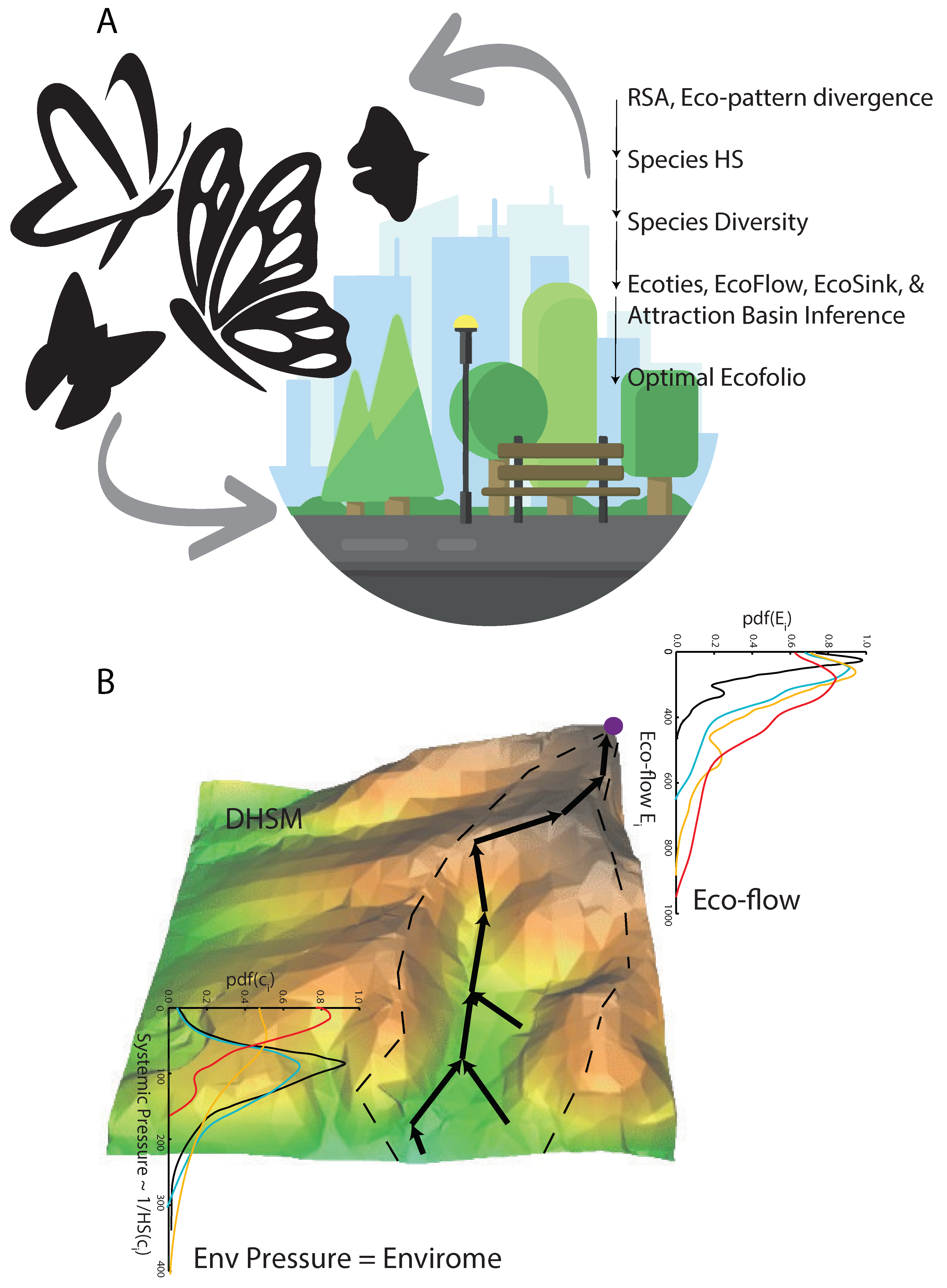
- Eco-functional networks and flows: From an eco-hydrological perspective, preferential eco-flow networks are defined by the connected steepest gradient paths of habitat suitability (HS) (Equation (2)) that offer the minimum resistance, approximating the flows of species across the landscape [61]. The cumulated flow, similar to the cumulated drainage area in hydrogeomorphology, approximates the potential cumulated abundance of species living on the landscape and moving along the preferential network [7,55]. This potential cumulated abundance provides a sense of the relative proportion of species in a landscape, considering all available preferential pathways.
- Eco-attraction basins: Eco-basins, equivalent to hydrological basins, are landscape areas where ecological flows converge into one network that is independent of others and reaches an ecological sink or outlet. Eco-basin boundaries (defining attraction basins and sinks that attract species from low to high climate-based HS) are defined by the maximum divergence between flows directed toward opposite directions (for one or more adjacent basins; see Equations (5) and (6)), independently of the magnitude of HS gradients. Eco-basin boundaries are equivalent to drainage divides in river basins. In a simpler geometrical definition, basin divides are defined by the curvature of HS that is greater than zero.
- Ecological sinks: Local ecological sinks are points where the HS gradient is the maximum (not necessarily points with the highest HS), and flows converge to these points. Therefore, ecological sinks are points along the ecological network (above a meaningful threshold on flows). Global eco-sinks are points with the highest HS gradient and HS (Equation (7)) toward where the vast majority of the flows converge. The outlet is often not the point with the largest HS. Often, the network diameter, which is the link with the shortest path to all other links (approximatively at the center of the network; see Convertino et al. [57]), is the global ecological sink.
4.2. Ecological Patterns and Systemic Fitness Indicators: Species as Hydroclimate Sentinels
4.3. Limitations and Perspectives
5. Conclusions
Author Contributions
Funding
Institutional Review Board Statement
Data Availability Statement
Acknowledgments
Conflicts of Interest
References
- Convertino, M.; Valverde, L.J., Jr. Toward a pluralistic conception of resilience. Ecol. Indic. 2019, 107, 105510. [Google Scholar] [CrossRef]
- Riva, F.; Graco-Roza, C.; Daskalova, G.N.; Hudgins, E.J.; Lewthwaite, J.M.M.; Newman, E.A.; Ryo, M.; Mammola, S. Toward a cohesive understanding of ecological complexity. Sci. Adv. 2023, 9, eabq4207. [Google Scholar] [CrossRef]
- Li, J.; Convertino, M. Inferring ecosystem networks as information flows. Sci. Rep. 2021, 11, 7094. [Google Scholar] [CrossRef]
- Funabashi, M. Human augmentation of ecosystems: Objectives for food production and science by 2045. npj Sci. Food 2018, 2, 16. [Google Scholar] [CrossRef]
- Funabashi, M. Power-law productivity of highly biodiverse agroecosystems supports land recovery and climate resilience. npj Sustain. Agric. 2024, 2, 8. [Google Scholar] [CrossRef]
- Rapport, D.J. Sustainability science: An ecohealth perspective. Sustain. Sci. 2007, 2, 77–84. [Google Scholar] [CrossRef]
- Rodriguez-Iturbe, I.; Muneepeerakul, R.; Bertuzzo, E.; Levin, S.A.; Rinaldo, A. River networks as ecological corridors: A complex systems perspective for integrating hydrologic, geomorphologic, and ecologic dynamics. Water Resour. Res. 2009, 45. [Google Scholar] [CrossRef]
- Li, J.; Convertino, M. Temperature increase drives critical slowing down of fish ecosystems. PLoS ONE 2021, 16, e0246222. [Google Scholar] [CrossRef]
- Wang, H.; Convertino, M. Algal bloom ties: Systemic biogeochemical stress and chlorophyll-a shift forecasting. Ecol. Indic. 2023, 154, 110760. [Google Scholar] [CrossRef]
- Zhang, J.; Convertino, M. Blueprinting the ecosystem health index for blue carbon ecotones. iScience 2024, 27, 111426. [Google Scholar] [CrossRef]
- Azaele, S.; Pigolotti, S.; Banavar, J.R.; Maritan, A. Dynamical evolution of ecosystems. Nature 2006, 444, 926–928. [Google Scholar] [CrossRef]
- Boguna, M.; Bonamassa, I.; De Domenico, M.; Havlin, S.; Krioukov, D.; Serrano, M. Network geometry. Nat. Rev. Phys. 2021, 3, 114–135. [Google Scholar] [CrossRef]
- Navarro, L.M.; Fernandez, N.; Guerra, C.; Guralnick, R.; Kissling, W.D.; Londoño, M.C.; Muller-Karger, F.; Turak, E.; Balvanera, P.; Costello, M.J.; et al. Monitoring biodiversity change through effective global coordination. Curr. Opin. Environ. Sustain. 2017, 29, 158–169. [Google Scholar] [CrossRef]
- Pereira, H.M.; Ferrier, S.; Walters, M.; Geller, G.N.; Jongman, R.H.G.; Scholes, R.J.; Bruford, M.W.; Brummitt, N.; Butchart, S.H.M.; Cardoso, A.C.; et al. Essential biodiversity variables. Science 2013, 339, 277–278. [Google Scholar] [CrossRef] [PubMed]
- Proença, V.; Martin, L.J.; Pereira, H.M.; Fernandez, M.; McRae, L.; Belnap, J.; Böhm, M.; Brummitt, N.; García-Moreno, J.; Gregory, R.D.; et al. Global biodiversity monitoring: From data sources to essential biodiversity variables. Biol. Conserv. 2017, 213, 256–263. [Google Scholar] [CrossRef]
- Braby, M.F.; Yeates, D.K.; Taylor, G.S. Population declines and the conservation of insects and other terrestrial invertebrates in australia. Austral Entomol. 2021, 60, 3. [Google Scholar] [CrossRef]
- Brown, J.; Threlfall, C.G.; Harrison, L.; Baumann, J.; Williams, N.S.G. Rapid responses of bees and butterflies but not birds to targeted urban road verge habitat enhancements. J. Appl. Ecol. 2024, 61, 1312–1322. [Google Scholar] [CrossRef]
- Brown, K.S.; Freitas, A.V.L. Butterfly communities of urban forest fragments in Campinas, São Paulo, Brazil: Structure, instability, environmental correlates, and conservation. J. Insect Conserv. 2002, 6, 217–231. [Google Scholar] [CrossRef]
- Kazemi, F.; Beecham, S.; Gibbs, J. Bioretention swales as multifunctional landscapes and their influence on australian urban biodiversity: Hymenoptera as biodiversity indicators. In Proceedings of the II International Conference on Landscape and Urban Horticulture, Bologna, Italy, 9–13 June 2009; Volume 881, pp. 221–227. [Google Scholar]
- Brose, U.; Hirt, M.R.; Ryser, R.; Rosenbaum, B.; Berti, E.; Gauzens, B.; Hein, A.M.; Pawar, S.; Schmidt, K.; Wootton, K.; et al. Embedding information flows within ecological networks. Nat. Ecol. Evol. 2025, 9, 547–558. [Google Scholar] [CrossRef]
- Krich, C.; Runge, J.; Miralles, D.G.; Migliavacca, M.; Perez-Priego, O.; El-Madany, T.; Carrara, A.; Mahecha, M.D. Estimating causal networks in biosphere–atmosphere interaction with the pcmci approach. Biogeosciences 2020, 17, 1033–1061. [Google Scholar] [CrossRef]
- Suzuki, K.; Matsuzaki, S.S.; Masuya, H. Decomposing predictability to identify dominant causal drivers in complex ecosystems. Proc. Natl. Acad. Sci. USA 2022, 119, e2204405119. [Google Scholar] [CrossRef]
- Harush, U.; Barzel, B. Dynamic patterns of information flow in complex networks. Nat. Commun. 2017, 8, 2181. [Google Scholar] [CrossRef] [PubMed]
- Peel, L.; Peixoto, T.P.; De Domenico, M. Statistical inference links data and theory in network science. Nat. Commun. 2022, 13, 6794. [Google Scholar] [CrossRef]
- Little, C.J.; Rizzuto, M.; Luhring, T.M.; Monk, J.D.; Nowicki, R.J.; Paseka, R.E.; Stegen, J.C.; Symons, C.C.; Taub, F.B.; Yen, J.D.L. Movement with meaning: Integrating information into meta-ecology. Oikos 2022, 2022, e08892. [Google Scholar] [CrossRef]
- Talluto, L.; Del Campo, R.; Estévez, E.; Altermatt, F.; Datry, T.; Singer, G. Towards (better) fluvial meta-ecosystem ecology: A research perspective. npj Biodivers. 2024, 3, 3. [Google Scholar] [CrossRef]
- Servadio, J.L.; Convertino, M. Optimal information networks: Application for data-driven integrated health in populations. Sci. Adv. 2018, 4, e1701088. [Google Scholar] [CrossRef] [PubMed]
- Holloway, P.; Miller, J.A. A quantitative synthesis of the movement concepts used within species distribution modelling. Ecol. Model. 2017, 356, 91–103. [Google Scholar] [CrossRef]
- Turney, E.K.; Goodrum, G.C.; Saunders, W.C.; Walsworth, T.E.; Null, S.E. Comparing commonly used aquatic habitat modeling methods for native fish. Ecol. Model. 2025, 499, 110909. [Google Scholar] [CrossRef]
- Liu, Y.; Hoppe, B.O.; Convertino, M. Threshold evaluation of emergency risk communication for health risks related to hazardous ambient temperature. Risk Anal. 2018, 38, 2208–2221. [Google Scholar] [CrossRef]
- Pekel, J.F.; Cottam, A.; Gorelick, N.; Belward, A.S. High-resolution mapping of global surface water and its long-term changes. Nature 2016, 540, 418–422. [Google Scholar] [CrossRef]
- Kuczynski, L.; Ontiveros, V.J.; Hillebrand, H. Biodiversity time series are biased towards increasing species richness in changing environments. Nat. Ecol. Evol. 2023, 7, 994–1001. [Google Scholar] [CrossRef] [PubMed]
- Sing, K.; Dong, H.; Wang, W.; Wilson, J.-J. Can butterflies cope with city life? butterfly diversity in a young megacity in southern china. Genome 2016, 59, 751–761. [Google Scholar] [CrossRef] [PubMed]
- Sing, K.; Luo, J.; Wang, W.; Jaturas, N.; Soga, M.; Yang, X.; Dong, H.; Wilson, J.-J. Ring roads and urban biodiversity: Distribution of butterflies in urban parks in beijing city and correlations with other indicator species. Sci. Rep. 2019, 9, 7653. [Google Scholar] [CrossRef]
- Lim, V.; Sing, K.; Chong, K.Y.; Jaturas, N.; Dong, H.; Lee, P.; Tao, N.T.; Le, D.T.; Bonebrake, T.C.; Tsang, T.P.N.; et al. Familiarity with, perceptions of and attitudes toward butterflies of urban park users in megacities across east and southeast asia. R. Soc. Open Sci. 2022, 9, 220161. [Google Scholar] [CrossRef]
- Wang, W.; Suman, D.O.; Zhang, H.; Xu, Z.; Ma, F.; Hu, S. Butterfly conservation in china: From science to action. Insects 2020, 11, 661. [Google Scholar] [CrossRef]
- McElderry, R.M.; de Lauriere, C.F.; Khoury, C.E.; Chaudhary, P.; Manu, S.; Specker, F.; Brettell, I.; Hoogen, J.v.; Maynard, D.; Lozano, C.B.; et al. Assessing the Multidimensional Complexity of Biodiversity Using a Globally Standardized Approach. 2023. Available online: https://ecoevorxiv.org/repository/view/5837/ (accessed on 28 March 2025).
- Hansen, A.; Barnett, K.; Jantz, P.; Phillips, L.; Goetz, S.J.; Hansen, M.; Venter, O.; Watson, J.E.M.; Burns, P.; Atkinson, S.; et al. Global humid tropics forest structural condition and forest structural integrity maps. Sci. Data 2019, 6, 232. [Google Scholar] [CrossRef]
- Grantham, H.S.; Duncan, A.; Evans, T.D.; Jones, K.R.; Beyer, H.L.; Schuster, R.; Walston, J.; Ray, J.C.; Robinson, J.G.; Callow, M.; et al. Anthropogenic modification of forests means only 40% of remaining forests have high ecosystem integrity. Nat. Commun. 2020, 11, 5978. [Google Scholar] [CrossRef] [PubMed]
- Galbraith, E.; Frade, P.R.; Convertino, M. Metabolic shifts of oceans: Summoning bacterial interactions. Ecol. Indic. 2022, 138, 108871. [Google Scholar] [CrossRef]
- Phillips, S.J.; Anderson, R.P.; Dudík, M.; Schapire, R.E.; Blair, M.E. Opening the black box: An open-source release of maxent. Ecography 2017, 40, 887–893. [Google Scholar] [CrossRef]
- Chowdhury, M.S.N.; Wijsman, J.W.M.; Hossain, M.S.; Ysebaert, T.; Smaal, A.C. A verified habitat suitability model for the intertidal rock oyster, saccostrea cucullata. PloS ONE 2019, 14, e0217688. [Google Scholar] [CrossRef]
- Convertino, M.; Annis, A.; Nardi, F. Information-theoretic portfolio decision model for optimal flood management. Environ. Model. Softw. 2019, 119, 258–274. [Google Scholar] [CrossRef]
- Convertino, M.; Troccoli, A.; Catani, F. Detecting fingerprints of landslide drivers: A maxent model. J. Geophys. Res. Solid Earth 2013, 118, 1367–1386. [Google Scholar] [CrossRef]
- Elith, J.; Phillips, S.J.; Hastie, T.; Dudík, M.; Chee, Y.E.; Yates, C.J. A statistical explanation of MaxEnt for ecologists. Divers. Distrib. 2010, 17, 43–57. [Google Scholar] [CrossRef]
- Merow, C.; Smith, M.J.; Silander, J.A., Jr. A practical guide to maxent for modeling species’ distributions: What it does, and why inputs and settings matter. Ecography 2013, 36, 1058–1069. [Google Scholar] [CrossRef]
- Phillips, S.; Anderson, R.; Schapire, R. Maximum entropy modeling of species geographic distributions. Ecol. Model. 2006, 190, 231–259. [Google Scholar] [CrossRef]
- Phillips, S.J.; Dudík, M. Modeling of species distributions with maxent: New extensions and a comprehensive evaluation. Ecography 2008, 31, 161–175. [Google Scholar] [CrossRef]
- Radosavljevic, A.; Anderson, R.P. Making better maxent models of species distributions: Complexity, overfitting and evaluation. J. Biogeogr. 2014, 41, 629–643. [Google Scholar] [CrossRef]
- Muscarella, R.; Galante, P.J.; Soley-Guardia, M.; Boria, R.A.; Kass, J.M.; Uriarte, M.; Anderson, R.P. Enm eval: An r package for conducting spatially independent evaluations and estimating optimal model complexity for maxent ecological niche models. Methods Ecol. Evol. 2014, 5, 1198–1205. [Google Scholar] [CrossRef]
- Convertino, M.; Muñoz-Carpena, R.; Chu-Agor, M.L.; Kiker, G.A.; Linkov, I. Untangling drivers of species distributions: Global sensitivity and uncertainty analyses of maxent. Environ. Model. Softw. 2014, 51, 296–309. [Google Scholar] [CrossRef]
- Tobón-Niedfeldt, W.; Mastretta-Yanes, A.; Urquiza-Haas, T.; Goettsch, B.; Cuervo-Robayo, A.P.; Urquiza-Haas, E.; Orjuela-R, M.A.; Gasman, F.A.; Oliveros-Galindo, O.; Burgeff, C.; et al. Incorporating evolutionary and threat processes into crop wild relatives conservation. Nat. Commun. 2022, 13, 6254. [Google Scholar] [CrossRef]
- Yackulic, C.B.; Chandler, R.; Zipkin, E.F.; Royle, J.A.; Nichols, J.D.; Grant, E.H.C.; Veran, S. Presence-only modelling using maxent: When can we trust the inferences? Methods Ecol. Evol. 2013, 4, 236–243. [Google Scholar] [CrossRef]
- Banavar, J.R.; Colaiori, F.; Flammini, A.; Maritan, A.; Rinaldo, A. Scaling, optimality, and landscape evolution. J. Stat. Phys. 2001, 104, 1–48. [Google Scholar]
- Rinaldo, A.; Gatto, M.; Rodríguez-Iturbe, I. River Networks as Ecological Corridors: Species, Populations, Pathogens; Cambridge University Press: Cambridge, UK, 2020. [Google Scholar]
- Banavar, J.R.; Cooke, T.J.; Rinaldo, A.; Maritan, A. Form, function, and evolution of living organisms. Proc. Natl. Acad. Sci. USA 2014, 111, 3332–3337. [Google Scholar] [CrossRef]
- Convertino, M.; Muneepeerakul, R.; Azaele, S.; Bertuzzo, E.; Rinaldo, A.; Rodriguez-Iturbe, I. On neutral metacommunity patterns of river basins at different scales of aggregation. Water Resour. Res. 2009, 45. [Google Scholar] [CrossRef]
- Liu, X.; Su, Y.; Li, Z.; Zhang, S. Constructing ecological security patterns based on ecosystem services trade-offs and ecological sensitivity: A case study of shenzhen metropolitan area, china. Ecol. Indic. 2023, 154, 110626. [Google Scholar] [CrossRef]
- Zhang, S.; Zhang, Z.; Wang, J.; Zhang, Y.; Wu, J.; Zhang, X. Effects of ecological control line on habitat connectivity: A case study of shenzhen, china. Ecol. Indic. 2024, 167, 112583. [Google Scholar] [CrossRef]
- Convertino, M.; Muñoz-Carpena, R.; Kiker, G.A.; Perz, S.G. Design of optimal ecosystem monitoring networks: Hotspot detection and biodiversity patterns. Stoch. Environ. Res. Risk Assess. 2015, 29, 1085–1101. [Google Scholar] [CrossRef]
- Wu, L.; Convertino, M. Ecological corridor design for ecoclimatic regulation: Species as eco-engineers. Ecol. Indic. 2025, 171, 113149. [Google Scholar] [CrossRef]
- Liu, J.; Costanza, R.; Kubiszewski, I.; Li, B.L.L.; Chen, F.; Day, J.W.; Gleick, P.H.; Makarieva, A.; McGlade, J.M.; Pimm, S.L.; et al. Zhengzhou 2024 ecosummit declaration: Building eco-civilization for a sustainable and desirable future. Ecol. Indic. 2025, 171, 113249. [Google Scholar]
- Rapport, D.J.; Costanza, R.; McMichael, A.J. Assessing ecosystem health. Trends Ecol. Evol. 1998, 13, 397–402. [Google Scholar]
- Liang, M.; Yang, Q.; Chase, J.M.; Isbell, F.; Loreau, M.; Schmid, B.; Seabloom, E.W.; Tilman, D.; Wang, S. Unifying spatial scaling laws of biodiversity and ecosystem stability. Science 2025, 387, eadl2373. [Google Scholar] [CrossRef] [PubMed]
- Liu, Y.; Liu, R.; Shang, R. Globmap swf: A global annual surface water cover frequency dataset during 2000–2020. Earth Syst. Sci. Data 2022, 14, 4505–4523. [Google Scholar] [CrossRef]
- Jung, M.; Dahal, P.R.; Butchart, S.H.M.; Donald, P.F.; Lamo, X.D.; Lesiv, M.; Kapos, V.; Rondinini, C.; Visconti, P. A global map of terrestrial habitat types. Sci. Data 2020, 7, 256. [Google Scholar] [CrossRef] [PubMed]


| Park Name | Abundance | Species Richness | Park Area (km2) | GPS Coordinates (N,E) | |
|---|---|---|---|---|---|
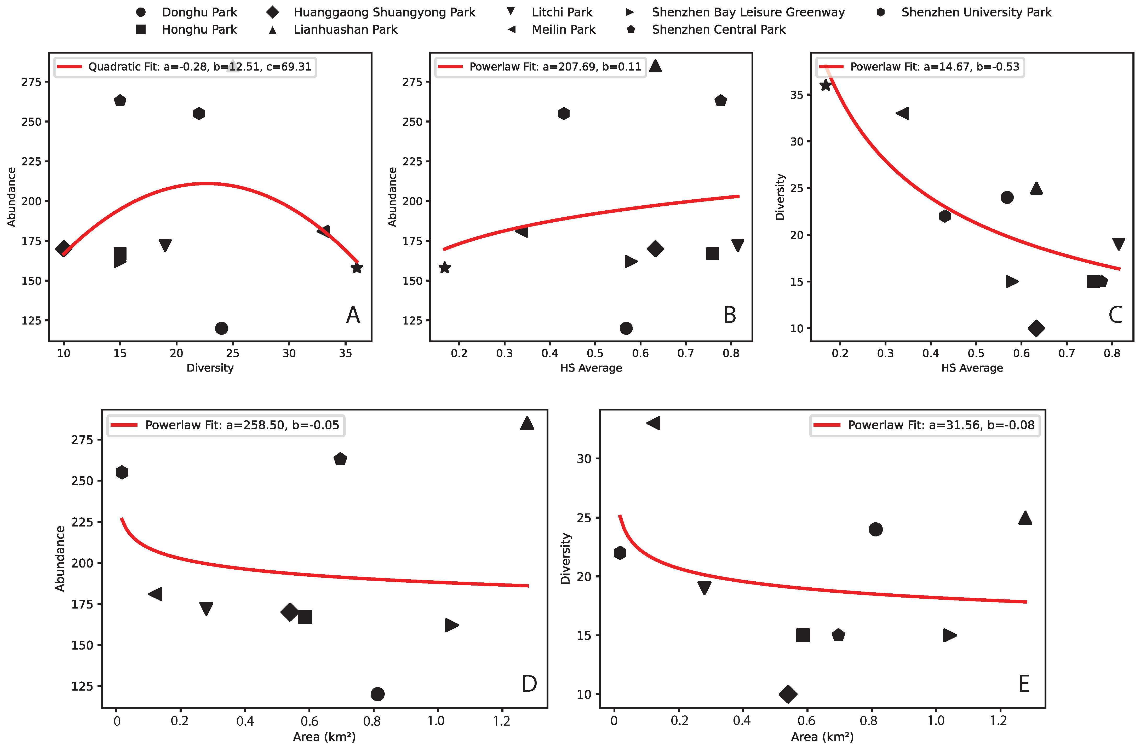
| Donghu Park | 120 | 24 | 0.81 | 0.57 | 22.588, 114.147 |
| Honghu Park | 167 | 15 | 0.59 | 0.76 | 22.569, 114.12 |
| Huanggaong Shuangyong Park | 170 | 10 | 0.54 | 0.63 | 22.552, 114.059 |
| Lianhuashan Park | 285 | 25 | 1.28 | 0.63 | 22.577, 114.058 |
| Litchi Park | 172 | 19 | 0.28 | 0.81 | 22.546, 114.102 |
| Meilin Park | 181 | 33 | 0.12 | 0.34 | 22.573, 114.036 |
| Shenzhen Bay Leisure Greenway | 162 | 15 | 1.04 | 0.58 | 22.522, 114.021 |
| Shenzhen Central Park | 263 | 15 | 0.70 | 0.78 | 22.551, 114.074 |
| Shenzhen University Park | 255 | 22 | 0.02 | 0.43 | 22.537, 113.931 |
| Tanglangshan Suburb Park | 158 | 36 | 41.09 | 0.17 | 22.574, 114.01 |
| Hydroclimatic Variables | Percentage Contribution | Permutation Importance |
|---|---|---|
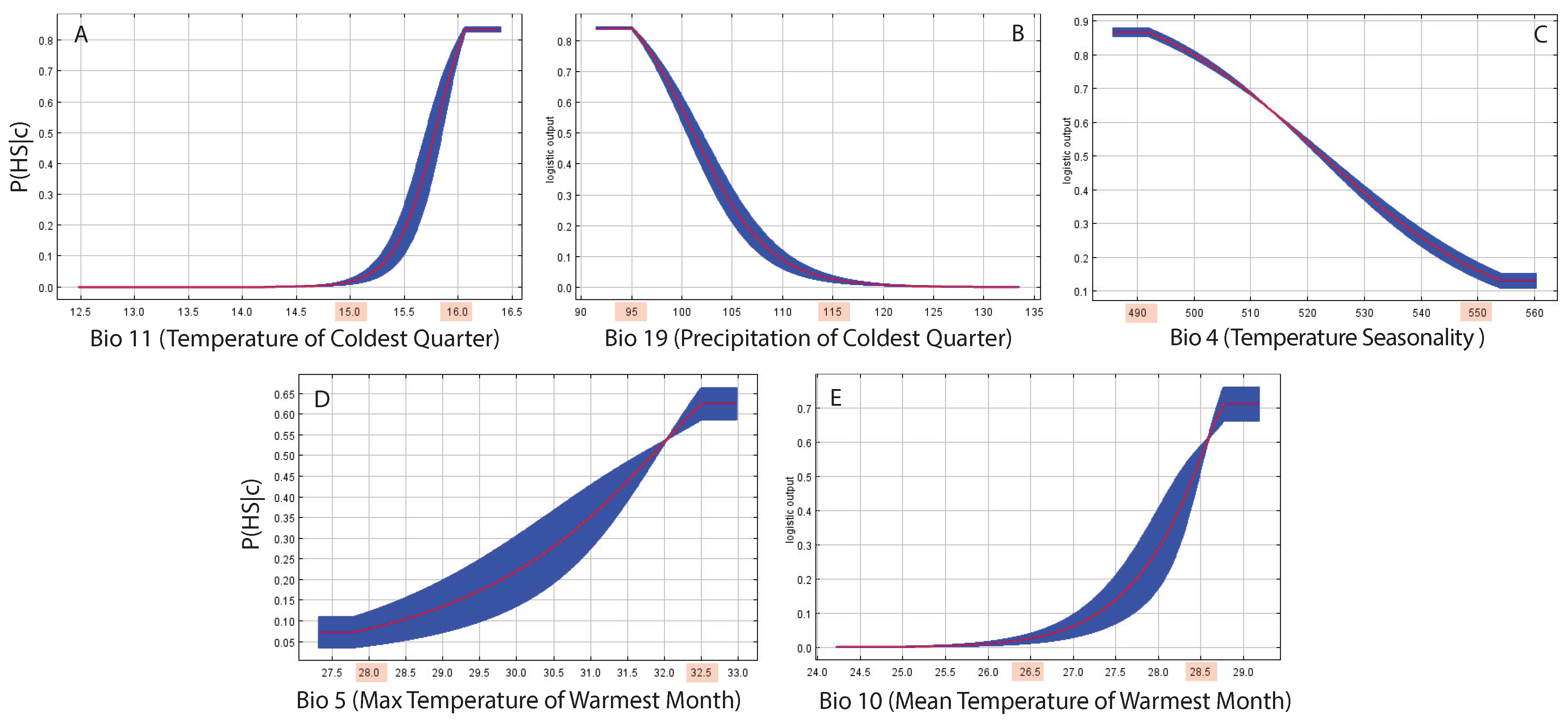
| BIO19: Precipitation of Coldest Quarter | 79.1 | 32.5 |
| BIO4: Temperature Seasonality (standard deviation ×100) | 6.5 | 18.6 |
| BIO11: Mean Temperature of Coldest Quarter | 5.2 | 37.2 |
| BIO6: Min Temperature of Coldest Month | 3.8 | 0.1 |
| BIO13: Precipitation of Wettest Month | 1.5 | 0 |
| BIO3: Isothermality (BIO2/BIO7) (×100) | 1 | 0.6 |
| BIO17: Precipitation of Driest Quarter | 0.8 | 0 |
| BIO9: Mean Temperature of Driest Quarter | 0.7 | 0 |
| BIO1: Annual Mean Temperature | 0.4 | 0 |
| BIO8: Mean Temperature of Wettest Quarter | 0.4 | 0 |
| BIO15: Precipitation Seasonality (Coefficient of Variation) | 0.3 | 0.5 |
| BIO5: Max Temperature of Warmest Month | 0.1 | 8.5 |
| BIO14: Precipitation of Driest Month | 0.1 | 0 |
| BIO7: Temperature Annual Range (BIO5-BIO6) | 0.1 | 0 |
| BIO10: Mean Temperature of Warmest Quarter | 0 | 1.9 |
| BIO18: Precipitation of Warmest Quarter | 0 | 0 |
| BIO16: Precipitation of Wettest Quarter | 0 | 0 |
| BIO12: Annual Precipitation | 0 | 0 |
| BIO2: Mean Diurnal Range (Mean of monthly (max temp - min temp)) | 0 | 0 |
Disclaimer/Publisher’s Note: The statements, opinions and data contained in all publications are solely those of the individual author(s) and contributor(s) and not of MDPI and/or the editor(s). MDPI and/or the editor(s) disclaim responsibility for any injury to people or property resulting from any ideas, methods, instructions or products referred to in the content. |
© 2025 by the authors. Licensee MDPI, Basel, Switzerland. This article is an open access article distributed under the terms and conditions of the Creative Commons Attribution (CC BY) license (https://creativecommons.org/licenses/by/4.0/).
Share and Cite
Convertino, M.; Wu, Y.; Dong, H. Baselining Urban Ecosystems from Sentinel Species: Fitness, Flows, and Sinks. Entropy 2025, 27, 486. https://doi.org/10.3390/e27050486
Convertino M, Wu Y, Dong H. Baselining Urban Ecosystems from Sentinel Species: Fitness, Flows, and Sinks. Entropy. 2025; 27(5):486. https://doi.org/10.3390/e27050486
Chicago/Turabian StyleConvertino, Matteo, Yuhan Wu, and Hui Dong. 2025. "Baselining Urban Ecosystems from Sentinel Species: Fitness, Flows, and Sinks" Entropy 27, no. 5: 486. https://doi.org/10.3390/e27050486
APA StyleConvertino, M., Wu, Y., & Dong, H. (2025). Baselining Urban Ecosystems from Sentinel Species: Fitness, Flows, and Sinks. Entropy, 27(5), 486. https://doi.org/10.3390/e27050486