Quantum κ-Entropy: A Quantum Computational Approach

Abstract

A novel approach to the quantum version of $\kappa$-entropy that incorporates it into the conceptual, mathematical and operational framework of quantum computation is put forward. Various alternative expressions stemming from its definition emphasizing computational and algorithmic aspects are worked out: First, for the case of canonical Gibbs states, it is shown that $\kappa$-entropy is cast in the form of an expectation value for an observable that is determined. Also, an operational method named “the two-temperatures protocol” is introduced that provides a way to obtain the $\kappa$-entropy in terms of the partition functions of two auxiliary Gibbs states with temperatures $\kappa$-shifted above, the hot-system, and $\kappa$-shifted below, the cold-system, with respect to the original system temperature. That protocol provides physical procedures for evaluating entropy for any $\kappa$. Second, two novel additional ways of expressing the $\kappa$-entropy are further introduced. One determined by a non-negativity definite quantum channel, with Kraus-like operator sum representation and its extension to a unitary dilation via a qubit ancilla. Another given as a simulation of the $\kappa$-entropy via the quantum circuit of a generalized version of the Hadamard test. Third, a simple inter-relation of the von Neumann entropy and the quantum $\kappa$-entropy is worked out and a bound of their difference is evaluated and interpreted. Also the effect on the $\kappa$-entropy of quantum noise, implemented as a random unitary quantum channel acting in the system’s density matrix, is addressed and a bound on the entropy, depending on the spectral properties of the noisy channel and the system’s density matrix, is evaluated. The results obtained amount to a quantum computational tool-box for the $\kappa$-entropy that enhances its applicability in practical problems.

1. Introduction

The $\kappa$-entropy introduced two decades ago in the trilogy of papers [1,2,3] assumes the form

$$S_{\kappa }={\displaystyle \frac{1}{2\kappa }}\sum _{i=1}^W\left({\rho }_i^{1-\kappa }-{\rho }_i^{1+\kappa }\right),$$

(1)

where $\rho =\left\{{\rho }_i\right\}$ is the probability density. The above entropy arises naturally in the context of Einstein’s special relativity and generates a self-consistent $\kappa$ statistical mechanics, which turns out to be a relativistic extension of classical Boltzmann–Gibbs statistical mechanics. which is obtained in the $\kappa \to 0$ classical limit.

The persistent power-law tails of the cosmic rays spectrum, spanning 13 decades in terms of energy and 33 decades in terms of particle flux, turn out to be a purely relativistic effect correctly predicted by $\kappa$ statistical mechanics and this result represents one of the greatest successes of the new theory.

The statistical theory based on $S_{\kappa }$ has an axiomatic structure and can also be introduced without reference to special relativity [4], since it also has applications outside of relativistic physics.

In the last two decades, many authors have studied the theoretical foundations of the underlying thermodynamics, [5,6,7,8,9,10,11,12,13] and the mathematical structure of the theory, c.f. [14,15,16,17,18,19,20,21,22,23,24,25,26].

On the other hand, specific applications of the theory have been considered in various areas of the science of complex physical, natural or artificial, classical or quantum systems. With regard to the applications concerning quantum systems, we recall the studies devoted in particular to quantum mechanics [27,28], quantum hadrodynamics [29], quantum statistical mechanics, c.f. [30,31,32], quantum gravity [33,34,35,36,37,38,39,40] and quantum cosmology, c.f. [41,42,43,44,45].

The content of the present paper frames the quantum version of $\kappa$-entropy and relates it to the conceptual, mathematical and operational framework of quantum computation. The relations developed are organized into three scopes, each one containing two propositions, that form the three main chapters of the paper, respectively. All proofs are deferred to a final Appendix A. The following outline describes the matter:

Scope 1: The aim is to consider a canonical Gibbs state density matrix for some Hamiltonian and determine an operational form for its kappa canonical quantum entropy via the expectation value of a quantum observable, Proposition 1; and further, to introduce a two-temperatures protocol for measuring the canonical state kappa entropy, Proposition 2.

Scope 2: The aim (channel generating kappa entropy) is to express the kappa entropy for a general density matrix via a positive and trace-preserving quantum channel as well as via its unitary dilation, Proposition 3; and further, to simulate the kappa entropy via a generalized form of the quantum circuit of the so-called Hadamard test, Proposition 4.

Scope 3: The aim is to relate the kappa and von Neumann quantum entropies between them and to determine the bounds on their difference, Proposition 5; and further, to examine the effect of a typical noise, i.e., a quantum random unitary channel acting on an original quantum system, by evaluating bounds on the value of the kappa entropy of the transformed density matrix. To gain full generality for the result, the bound is shown to be determined by the spectral properties of both the channel and systems’ density matrix, Proposition 6.

Motivations:$\kappa$-Entropy and its relations to other quantum entropies: Some of the motivation for the development of $\kappa$ entropy in quantum information language is based on its relation to other standard quantum entropies, such as von Neumann (vNE) and Renyi entropy. Operational interpretations of vNE supporting its wide use in the quantum information field are well known, and two of them are invoked below. Here, they are useful in motivating a similar interpretation for the quantum $\kappa$ entropy, c.f. Proposition 2 below. Similarly to vNE, the Renyi entropy shares common features with $\kappa$ entropy, supporting the treatment of the latter in quantum language as outlined below.

vN entropy intepretation 1: Suppose that Alice prepares a quantum state $\rho$. Bob can then perform a particular POVM ${\left\{{\mathrm{\Lambda }}_x\right\}}_{x\in \mathcal{X}}$ to learn about the quantum system, where X denotes the random variable corresponding to the classical output of the POVM, i.e., $x\to {\mathrm{\Lambda }}_x$. The probability density function $x\to p_X\left(x\right)$ of random variable X is then $p_X\left(x\right)=Tr\left(\rho {\mathrm{\Lambda }}_x\right).$ The Shannon entropy of the POVM ${\mathrm{\Lambda }}_x$ is denoted by $S_{sh}\left(X\right)=-{\sum }_{x\in \mathcal{X}}{p}_X\left(x\right)log\left(p_X\left(x\right)\right)=-{\sum }_{x\in \mathcal{X}}Tr\left(\rho {\mathrm{\Lambda }}_x\right)log\left(Tr\left(\rho {\mathrm{\Lambda }}_x\right)\right).$ The minimum Shannon entropy over all rank-1 POVMs is equal to a quantity which is identified with the von Neumann entropy $S_{vN}\left(\rho \right)$ of the density operator $\rho .$ Explicitly, this optimization means that $S_{vN}\left(\rho \right)={min}_{\left\{{\mathrm{\Lambda }}_x\right\}}\left\{-{\sum }_{x\in \mathcal{X}}Tr\left(\rho {\mathrm{\Lambda }}_x\right)log\left(Tr\left(\rho {\mathrm{\Lambda }}_x\right)\right)\right\},$ where the minimum is restricted to be over rank-1 POVMs, i.e., those with $\{{\mathrm{\Lambda }}_x=|{\psi }_x〉〈{\psi }_x{\left|\right\}}_{x\in \mathcal{X}},$ satisfying ${\sum }_{x\in \mathcal{X}}{\mathrm{\Lambda }}_x={\sum }_{x\in \mathcal{X}}\left|{\psi }_x〉〈{\psi }_x\right|=\mathbb{I},$ where the latter implies the completeness of states ${\left\{\right|{\psi }_x〉\}}_{x\in \mathcal{X}}$ (p. 256, [46]).

vN entropy intepretation 2: Suppose that Alice generates a quantum state $|{\psi }_x〉$ in her lab according to some probability density $p_X\left(x\right)$ of a random variable X. Suppose further that Bob has not yet received the state from Alice and does not know which one she sent. The expected density operator from Bob’s point of view is then $\rho ={\mathbb{E}}_X\left\{|{\psi }_x〉〈{\psi }_x|\right\}={\sum }_{x\in \mathcal{X}}{p}_X\left(x\right)\left|{\psi }_x〉〈{\psi }_x\right|.$ The interpretation of the entropy $S_{vN}\left(\rho \right)$ is that it quantifies Bob’s uncertainty about the state Alice sent—his expected information gain is $S_{vN}\left(\rho \right)$ qubits upon receiving and measuring the state that Alice sends (p. 254, [46]).

Remark: The development of $\kappa$ entropy along the lines of quantum information put forward in this paper opens the possibility of using it to quantify, e.g., quantum entanglement, a procedure that has been carried out by other types of entropy, c.f. the entanglement Renyi $\alpha$-entropy (ERαE) index, c.f. [47] and references therein. Below an outline of the important features of Renyi $\alpha$-entropy and their comparison with those of $\kappa$ entropy is provided that supports this line of inquiry [48].

Renyi and $\kappa$ entropy: The presence of a logarithm function of the probability density in the expression of the von Neumann entropy $-Tr(\rho ln\rho )$ implies that the entropy calculation requires the computation of the complete spectrum of the density matrix for its diagonalization, which can be computationally intensive for large systems. The Renyi entropy ${\displaystyle \frac{1}{1-\alpha }}ln\left(Tr{\rho }^{\alpha }\right)$ instead involves a power of the probability density and is often computationally easier to estimate than the von Neumann entropy. As a result, the Renyi entropy is much more efficient and accessible for simulating complex quantum systems, as it relies on power traces rather than full eigenvalue decompositions of the von Neumann entropy, leading to faster and more scalable simulations.

The Renyi entropy is very flexible and depends on a free parameter that controls the entropy value. This allows more flexible forms and different weighting schemes of the probability distribution to be considered.

An important advantage of the variability of the free Renyi parameter is that by fixing it appropriately, the entropy measure can emphasize different aspects of the probability distribution of a quantum state by focusing on the most probable components or on the less dominant contributions to better understand the complex nature of the entanglement and quantum correlations. This versatility of the Renyi entropy can be particularly beneficial in the study of critical phenomena where certain entanglement features might be obscured by a single, fixed measure, or in phenomena where entanglement scaling and phase transitions reveal subtle quantum effects.

The Renyi entropy may be more accessible in experimental and computational settings than techniques such as interference-based measurements. The advantages of the Renyi entropy over the von Neumann entropy not only allow us to better characterize quantum states and gain deeper insights into the distribution and exchange of information between entangled particles, but also to improve error analysis and algorithm optimization in quantum computing.

The properties of the Renyi entropy, which make it faster to compute and more flexible than the von Neumann entropy, are due to its expression and, in particular, its dependence on a power of the probability density with a free parameter as the exponent. Of course, other entropies have also been considered in the literature, which share with the Renyi entropy the fact that they are also constructed from powers of the probability density and therefore share the main qualitative properties of the Renyi entropy. The choice of an entropy that generalizes the von Neumann entropy and uses powers instead of the logarithm of the probability density in its definition is very difficult and subjective.

Here, the $\kappa$-entropy is considered as a new paradigm of quantum entropy for two different reasons. The first is that the $\kappa$-entropy, like the Renyi entropy, is defined from the power of the probability density and thus shares the main qualitative features of the Renyi entropy. The second reason for choosing the $\kappa$-entropy, which makes it more interesting, is that it has a physical origin. The $\kappa$ parameter of entropy has its roots in Einstein’s theory of special relativity. It is a relativistic generalization of the Boltzmann entropy of classical statistical mechanics and thus of the von Neumann quantum entropy. The $\kappa$-entropy can therefore be seen as the relativistic generalization of the von Neumann entropy, which results when the parameter $\kappa$ approaches zero. The study of $\kappa$-entropy in the context of quantum computing and quantum information therefore allows us to consider quantum systems that have relativistic properties. This gives us a more comprehensive view of the nature of quantum-relativistic phenomena.

2. Kappa Entropy for Canonical States

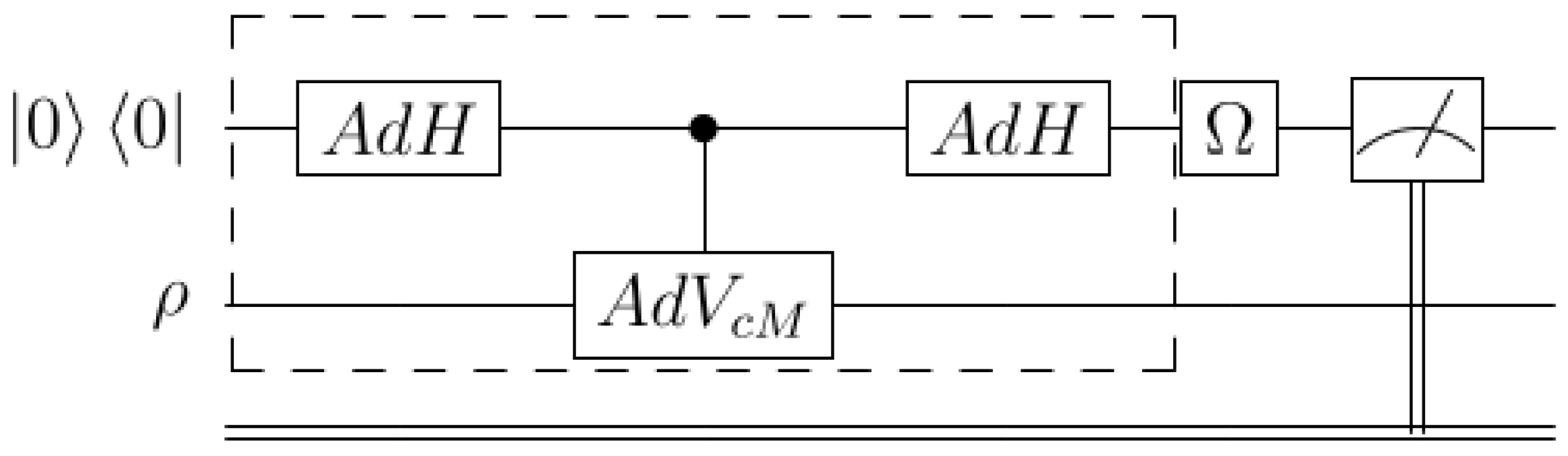
The aim of this section is to consider a canonical Gibbs state density matrix for some Hamiltonian and determine an operational form for its kappa canonical quantum entropy via the expectation value of a quantum observable, Proposition 1; and further, to introduce a two-temperatures protocol for measuring the canonical state kappa entropy of a give quantum system, Proposition 2. Consider the following,

Definition 1.

Let $\kappa \in [0,1)$ and let the density $\rho \in {\mathcal{D}}_N=\left\{\rho \in {\mathbb{C}}^{N\times N};{\rho }^{†}=\rho ,\rho >0,Tr\rho =1\right\},$ the kappa entropy reads

$$S_{\kappa }\left(\rho \right)=-{\displaystyle \frac{1}{2\kappa }}Tr({\rho }^{\kappa +1}-{\rho }^{-\kappa +1})$$

$\kappa +1\in [1,2),-\kappa +1\in [1,0).$

Next, we show how the canonical state kappa entropy is expressed via the expectation value of a quantum observable.

Proposition 1.

The kappa entropy of a canonical state ${\rho }_{can}={\displaystyle \frac{1}{Z_T}}{e}^{-\beta H},$$\beta ={\displaystyle \frac{1}{kT}},$ is cast in the form of an expectation value of the measurement of the quantum observable $C_{\kappa }={\displaystyle \frac{1}{\kappa }}sinh\left(\kappa (ln{Z}_T\mathbb{I}+\beta H)\right)$, in state ${\rho }_{can}$, i.e.,

$$S_{\kappa }\left({\rho }_{can}\right)=-Tr\left({\rho }_{can}{C}_{\kappa }\right)=-〈{\rho }_{can},C_{\kappa }〉.$$

State and observable are commuting.

Next, we put forward a two-temperatures protocol for measuring the canonical state kappa entropy,

Proposition 2.

The kappa entropy of a canonical state ${\rho }_{can}={\displaystyle \frac{1}{Z_T}}{e}^{-\beta H}$ of temperature $T,$ and partition function $Z_T=Tr\left(e^{-\beta H}\right),$ is simulated by two quantum systems described by the same Hamiltonian each in the canonical Gibbs state of the respective κ-dependent temperatures $T_{cool}={\displaystyle \frac{T}{1+\kappa }}<T$ (the cool system) and $T_{hot}={\displaystyle \frac{T}{1-\kappa }}>T$ (the hot system), with corresponding partition functions $Z_{cool}\equiv Z_{{\displaystyle \frac{T}{1+\kappa }}}$ and $Z_{hot}\equiv Z_{{\displaystyle \frac{T}{1-\kappa }}}.$ The kappa entropy is expressed in terms of the partition functions of the simulating systems as

$$S_{\kappa }\left({\rho }_{can}\right)=-{\displaystyle \frac{1}{2\kappa }}{\displaystyle \frac{1}{Z_T}}\left(Z_{{\displaystyle \frac{T}{1+\kappa }}}\times {\displaystyle \frac{1}{Z_T^{\kappa }}}-Z_{{\displaystyle \frac{T}{1-\kappa }}}\times Z_T^{\kappa }\right).$$

(2)

The protocol: For a given canonical density matrix ${\rho }_{can}$ with given Hamiltonian H and reference temperature $\beta ={\displaystyle \frac{1}{kT}}$, apply the following two-temperatures protocol in order to determine the kappa entropy $S_{\kappa }\left({\rho }_{can}\right)$. Suppose the $\kappa$ parameter is fixed and not adjustable, then introduce and control two temperatures: the high $T_{hot}\equiv T_{-\kappa }={\displaystyle \frac{T}{1-\kappa }}$ and the low $T_{cool}\equiv T_{+\kappa }={\displaystyle \frac{T}{1+\kappa }}$ temperatures, lying above and below the reference temperature T. By varying the high-T and the low-T temperature independently and determining the partition functions indicated in the last Equation (2), it is possible to simulate the value of the kappa entropy of the initial Gibbs state for any value of T and $\kappa .$ Operationally, that would require letting two copies of the original system of temperature T interact with a heat bath that will increase its temperature $T\to$$T_{hot}={\displaystyle \frac{T}{1-\kappa }}$ in the first copy and decrease its temperature $T\to T_{cool}={\displaystyle \frac{T}{1+\kappa }}$ in the second copy, and then form the combination of the partition function expressed in Equation (2).

3. Quantum Channels for $\kappa$ Entropy

The aim of this section is to express the kappa entropy for a general density matrix via a positive and trace-preserving quantum channel as well as via its unitary dilation, Proposition 3 [49,50,51,52]; and further, to simulate the kappa entropy via a generalized form of the quantum circuit of the so-called Hadamard test, [53], Proposition 4. We introduce the following:

Proposition 3.

By means of the formalism of the vectorization of matrices $A\to \left|A〉\right.〉$ and the purification of the density matrices $\rho \to \left|\sqrt{\rho }〉\right.〉,$ the κ entropy $S_{\kappa }$ is expressed as

$$S_{\kappa }\left(\rho \right)=Tr\left(T{r}_2{\mathcal{E}}_{\rho }\left(\left|\mathbb{I}〉\right.〉\left.〈〈\mathbb{I}\right|\right)\right),$$

where for any $\nu \in {\mathbb{C}}^{N\times N}\otimes {\mathbb{C}}^{N\times N}$, the positive semi-definite map ${\mathcal{E}}_{\rho }:{\mathbb{C}}^{N\times N}\otimes {\mathbb{C}}^{N\times N}\to {\mathbb{C}}^{N\times N}\otimes {\mathbb{C}}^{N\times N},$ is introduced as, ${\mathcal{E}}_{\rho }\left(\nu \right)=R_{+}\left(\rho \right)\nu R_{+}\left(\rho \right)-R_{-}\left(\rho \right)\nu R_{-}\left(\rho \right)$, with (Kraus-like) generators

$$R_{\pm }\left(\rho \right)={\displaystyle \frac{1}{\sqrt{\kappa }}}({\rho }^{{\displaystyle \frac{\pm \kappa +1}{2}}}\otimes \mathbb{I}).$$

Map ${\mathcal{E}}_{\rho }$ is also expressed in an extended space, by adding an auxiliary qubit. The density matrix of the total, auxiliary+system, is defined on matrix space ${\mathbb{C}}^{2\times 2}\otimes {\mathbb{C}}^{N\times N}\otimes {\mathbb{C}}^{N\times N}.$ Map ${\mathcal{E}}_{\rho }$ is explicitly obtained as

$${\mathcal{E}}_{\rho }\left(\nu \right)=T{r}_1\left(U\left(\rho \right){\sigma }_3\otimes \nu U^{†}\left(\rho \right)\right)$$

where the channel reads

$${\mathcal{E}}_{\rho }\left(\nu \right)=T{r}_1\left(\begin{array}{c}{\displaystyle \frac{1}{\sqrt{\kappa }}}{R}_{+}\left(\rho \right)\\ & {\displaystyle \frac{1}{\sqrt{\kappa }}}{R}_{-}\left(\rho \right)\end{array}\right)\left(\begin{array}{c}\nu \\ & -\nu \end{array}\right){\left(\begin{array}{c}{\displaystyle \frac{1}{\sqrt{\kappa }}}{R}_{+}\left(\rho \right)\\ & {\displaystyle \frac{1}{\sqrt{\kappa }}}{R}_{-}\left(\rho \right)\end{array}\right)}^{†}.$$

Kappa entropy via generalized Hadamard test circuit:

Devise an operational construction which will enable the implementation of the transformation ${\rho }^{\pm \kappa }\to {\rho }^{1\pm \kappa },$ and further generate the quantity $S_{\kappa }$. To this end, next, we provide a quantum measurement procedure that evaluates the trace $Tr{\rho }^{1\pm \kappa },$ that is based on an extension to the density matrix formalism of the idea of the so-called ’Hadamard test’, initially used for pure states (see, e.g., [53]). The quantum circuit of the proposed measurement is given below.

Notation: $AdX$ stands for the adjoint action of operator $X\in {\mathbb{C}}^{N\times N},$ as follows $AdX(.)=X(.)X^{†}.$ E.g., let the control X gate $V_{cX}=P_0\otimes X+P_1\otimes {\mathbb{I}}_N,$ acting on the composite system with control on the qubit state and target on the reference system; the notation $Ad{V}_{cX}$ means the adjoint action, i.e.,

$$Ad{V}_{cX}(.)=V_{cX}(.)V_{cX}^{†}=\left(P_0\otimes X+P_1\otimes \mathbb{I}\right)(.)\left(P_0\otimes X^{†}+P_1\otimes \mathbb{I}\right).$$

Simulation of kappa entropy via generalized Hadamard test quantum circuit (Proposition 4; c.f. Figure 1).

Proposition 4.

Consider attaching to the Hilbert space ${\mathbb{C}}^N$ of the reference quantum system, an auxiliary qubit so that the total state space is $\mathcal{H}\approx {\mathbb{C}}^2\otimes {\mathbb{C}}^N.$ Next, consider the initial state $\left|0\right.〉\left.〈0\right|\otimes \rho ,$ where we denote by ρ the density matrix of the system for which we want to evaluate the kappa entropy. For a matrix $M\in End\left({\mathbb{C}}^N\right)\approx {\mathbb{C}}^{N\times N},$ introduce the following map $\mathcal{S}\left[M\right]:\mathcal{D}\left(\mathcal{H}\right)\to \mathcal{D}\left(\mathcal{H}\right)$ in the space of the density matrices $\mathcal{D}\left(\mathcal{H}\right)\approx \mathcal{D}({\mathbb{C}}^2\otimes {\mathbb{C}}^N);$ explicitly, for H as the Hadamard matrix, the map $\mathcal{S}\left[M\right]$ is determined by composing the transformations $AdH\otimes {\mathbb{I}}_N$ and $Ad{V}_{cM},$ where both of them operate on the composite system of reference+qubit, and reads,

$$\mathcal{S}\left[M\right]\equiv \left(AdH\otimes {\mathbb{I}}_N\right)\circ Ad{V}_{cM}\circ \left(AdH\otimes {\mathbb{I}}_N\right).$$

For Ω and $M,$ operators on the auxiliary qubit and the reference systems, respectively, define the map $M\to {\mathcal{T}}_{\mathrm{\Omega }}\left[M\right],$

$${\mathcal{T}}_{\mathrm{\Omega }}\left[M\right]\equiv T{r}_1\left\{(\mathrm{\Omega }\otimes {\mathbb{I}}_N)\circ \mathcal{S}\left[M\right]\right\}:\mathcal{D}\left(\mathcal{H}\right)\to \mathcal{D}\left(\mathcal{H}\right),$$

parametrized by some Ω and $M.$ Acting on an initial state $\left|0\right.〉\left.〈0\right|\otimes \rho ,$ map ${\mathcal{T}}_{\mathrm{\Omega }}\left[M\right]$ yields ${\mathcal{T}}_{\pm {\sigma }_3}\left[{\rho }^{\pm \kappa }\right]=\pm {\rho }^{1\pm \kappa }.$ Denoting ${\mathcal{T}}_{\pm {\sigma }_3}\equiv$${\mathcal{T}}_{\pm }$ the kappa entropy $S_{\kappa }\left(\rho \right)$ is generated acting on $\left|0\right.〉\left.〈0\right|\otimes \rho$ as

$$\begin{array}{cc}& Tr\left[{\displaystyle \frac{1}{2\kappa }}\left({\mathcal{T}}_{+}\left[{\rho }^{\kappa }\right]+{\mathcal{T}}_{-}\left[{\rho }^{-\kappa }\right]\right)(\left|0\right.〉\left.〈0\right|\otimes \rho )\right]\hfill \\ =& -{\displaystyle \frac{1}{2\kappa }}Tr\left[\left({\rho }^{1+\kappa }-{\rho }^{1-\kappa }\right)\right]\hfill \\ =& S_{\kappa }\left(\rho \right).\hfill \end{array}$$

4. Set of Values and Bounds for $\kappa$ Entropy

In this section, two questions are investigated: (i) What is the set of values of a (scaled) difference between the von Neumann and $\kappa$ entropy (Proposition 6)?; and (ii) If an input density matrix is transformed by a unitary quantum channel, how is the output density matrix $\kappa$-entropy $S_{\kappa }$ affected? Explicit upper bounds on $S_{\kappa }$ are estimated that are determined by the stochastic properties of the channel generators, as well as by the spectral properties of the input-output density matrices, (Proposition 6).

Proposition 5.

The κ quantum entropy within the validity of function $sinh{c}_{\pi }$ approximation, [54,55,56,57], is

$$S_{\kappa }\left(\rho \right)=S_{vN}\left(\rho \right)-\underset{n\to \infty }{lim}Tr\left(\rho ln\rho \sum _{m=1}^n{\displaystyle \frac{1}{(2m+1)!}}{\left(\pi \kappa ln\rho \right)}^{2m}\right)$$

(3)

so it reads as a κ-depended correction to the von Neumann quantum entropy.

The following bounds are applied for the kappa entropy in terms of the vN entropy:

$$\begin{array}{ccc}\hfill S_{\kappa }\left(\rho \right)& \ge & S_{vN}\left(\rho \right)-\left(\underset{n\to \infty }{lim}{\displaystyle \frac{n}{(2n+1)!}}{\lambda }_{min}^n\right)〈u_{max}\left|\left(\mathrm{\Lambda }\left|ln\mathrm{\Lambda }\right|\right)\right|u_{max}〉\hfill \\ \hfill S_{\kappa }\left(\rho \right)& \le & S_{vN}\left(\rho \right)-\left(\underset{n\to \infty }{lim}{\displaystyle \frac{n}{6}}{\lambda }_{max}\right)〈u_{max}|\left(\mathrm{\Lambda }\left|ln\mathrm{\Lambda }\right|\right)\left|u_{max}〉\right).\hfill \end{array}$$

Also, in terms of the maximal eigenvalue and eigenvector of $\left|ln\rho \right|$ and by virtue of the Perron–Frobenius theorem, it is found that in the asymptotic limit ($n\to \infty )$, the scaled difference of the two entropies has the interval of values:

$${\displaystyle \frac{S_{\kappa }\left(\rho \right)-S_{vN}\left(\rho \right)}{〈u_{max}|\left(\mathrm{\Lambda }\left|ln\mathrm{\Lambda }\right|\right)\left|u_{max}〉\right)}}\in [0,\infty ).$$

Bounded change of the kappa entropy due to quantum random unitary channel (Proposition 6) (see [58,59,60]):

Proposition 6.

Let a quantum random unitary channel $\mathcal{E}$ that induces a transformation of $\rho \to {\rho }^{\prime }=\mathcal{E}\left(\rho \right)={\sum }_i{p}_i{A}_i\rho A_i^{†},$ with $A_i$ be its unitary generators and $p=\left(p_i\right)$ the vector of its weights. Also, let $\lambda ,{\lambda }^{\prime }$ be the eigenvalue stochastic vectors of ρ and the ${\rho }^{\prime }$ density matrices, respectively. The transformed density matrix is used together with the channel to derive or estimate the κ-entropy. Its components ${\rho }^{\prime \pm \kappa +1}$ are bounded by bounds determined by the spectral parameters of the input density matrix, and by the spectral and stochastic parameters of the channel as follows:

$$\begin{array}{ccc}\hfill Tr{\rho }^{\prime \kappa +1}& \le & {\eta }_{\kappa }{\left(∥\left|p\right.〉∥∥\left|\lambda \right.〉∥\right)}^{\kappa +1},\hfill \\ \hfill Tr{\rho }^{\prime -\kappa +1}& \le & {\eta }_{-\kappa }{\left(∥\left|p\right.〉∥∥\left|\lambda \right.〉∥\right)}^{-\kappa +1}.\hfill \end{array}$$

In the proof, the variable ${\eta }_{\kappa }={\sum }_i{\left(\sqrt{Tr{H}^{\left(i\right)}{H}^{\left(i\right)T}}\right)}^{\kappa +1}$ has been introduced, where the matrices $H_{jm}^{\left(i\right)}\equiv {\left(h^j\right)}_{im},$ and the circulant permutation $h|n〉=|n+1〉,\mathrm{mod}N,$ have been used along with the following lemma [61,62,63,64]:

Lemma 1.

Let the quantum random unitary channel transformation of $\rho \to {\rho }^{\prime }=\mathcal{E}\left(\rho \right)={\sum }_i{p}_i{A}_i\rho A_i^{†},$ with $A_i$ be unitary. Let $\lambda ,{\lambda }^{\prime }$ be the eigenvalue vectors of the ρ and ${\rho }^{\prime }$ density matrices, respectively, which are related by the unistochastic matrix ${\mathrm{\Delta }}_{\mathcal{E}}={\sum }_i{p}_i{A}_i\circ A_i^{\ast },$ as ${\lambda }^{\prime }={\mathrm{\Delta }}_{\mathcal{E}}\lambda .$ If, via Birkhoff’s theorem, the bi-stochastic matrix ${\mathrm{\Delta }}_{\mathcal{E}}$ is decomposed as a convex combination of circular permutations $\left\{h^i\right\},$ then ${\mathrm{\Delta }}_{\mathcal{E}}={\sum }_i{p}_i{h}^i$.

5. Summary and Outlook

The material covered in this paper provides tools and concepts from the field of quantum computation-information in order to enable a useful interaction with the theory of kappa entropy. The canonical state kappa entropy is shown to offer a framework where quantum computing would inspire operational methods for analyzing further the kappa entropy and motivate quantum mechanical measurements based on the entropy. Similarly, the quantum channel formalism and the constructive method of the Hadamard circuit that have been developed for $\kappa$ entropy transformation and generation reveal an intimate relation of those techniques with entropy, and applications along those lines would be anticipated. Finally, the interrelations between the von Neumann entropy and $\kappa$ entropy place the latter within the broad field of entropies, a fact that would enable the $\kappa$ entropy to be applied in the fields of open quantum systems and master equations. Finally, we mention some specific research topics that the formalism put forward here could help investigate. Examples are as follows: (i) How does the $\kappa$ entropy evolve in time for the density matrix of a qubit system evolving temporally by means of a time-dependent unitary evolution channel with a Kraus generator governed by a propagator determined by a coherent state path integral $SU\left(2\right)\setminus SU(1,1)$? [65]. (ii) How can the $\kappa$ entropy quantify the entanglement developed among the coin system and the walker system in the course of diffusion of an anyonic quantum walk? [66]. (iii) A similar question to (i) but now with a Kraus generator governed by the Hamiltonian of a qubit that has developed a Berry adiabatic geometric phase in the framework of sudden-adiabatic approximation [67]. Also, unlike the three previous dynamic studies, a novel kinematical study for $\kappa$ entropy is suggested. How does the $\kappa$ entropy of a bipartite quantum system of a composite number dimension d, e.g., $d=6,$ change if the parent system decomposes naturally based on the so-called prime-decomposition, and splits into two subsystems of dimension $d_A=2$ (qubit) and $d_B=3$ (qutrit)? [64]. Finally, addressing questions related to the relativistic origin and aspects of $\kappa$ entropy, [4], is an interesting, open area that would benefit from the present formalism.

References

1. Kaniadakis, G. Non-linear kinetics underlying generalized statistics. Phys. A 2001, 296, 405–425. [Google Scholar] [CrossRef]
2. Kaniadakis, G. Statistical mechanics in the context of special relativity. Phys. Rev. E 2002, 66, 056125. [Google Scholar] [CrossRef] [PubMed]
3. Kaniadakis, G. Statistical mechanics in the context of special relativity II. Phys. Rev. E 2005, 72, 036108. [Google Scholar] [CrossRef] [PubMed]
4. Kaniadakis, G. Relativistic roots of κ-entropy. Entropy 2024, 26, 406. [Google Scholar] [CrossRef]
5. Silva, R. The relativistic statistical theory and Kaniadakis entropy: An approach through a molecular chaos hypothesis. Eur. Phys. J. B 2006, 54, 499–502. [Google Scholar] [CrossRef]
6. Silva, R. The H-theorem in κ-statistics: Influence on the molecular chaos hypothesis. Phys. Lett. A 2006, 352, 17–20. [Google Scholar] [CrossRef]
7. Wada, T. Thermodynamic stabilities of the generalized Boltzmann entropies. Phys. A 2004, 340, 126–130. [Google Scholar]
8. Wada, T. Thermodynamic stability conditions for nonadditive composable entropies. Contin. Mechan. Thermod. 2004, 16, 263–267. [Google Scholar] [CrossRef]
9. Naudts, J. Deformed exponentials and logarithms in generalized thermostatistics. Phys. A 2002, 316, 323–334. [Google Scholar] [CrossRef]
10. Naudts, J. Continuity of a class of entropies and relative entropies. Rev. Math. Phys. 2004, 16, 809–822. [Google Scholar] [CrossRef]
11. Scarfone, A.M.; Wada, T. Canonical partition function for anomalous systems described by the κ-entropy. Prog. Theor. Phys. Suppl. 2006, 162, 45–52. [Google Scholar] [CrossRef]
12. Yamano, T. On the laws of thermodynamics from the escort average and on the uniqueness of statistical factors. Phys. Lett. A 2003, 308, 364–368. [Google Scholar] [CrossRef]
13. Lucia, U. Maximum entropy generation and kappa-exponential model. Phys. A 2010, 389, 4558–4563. [Google Scholar] [CrossRef]
14. Pistone, G. κ-exponential models from the geometrical point of view. Eur. Phys. J. B 2009, 70, 29–37. [Google Scholar] [CrossRef]
15. Pistone, G.; Shoaib, M. Kaniadakis’s Information Geometry of Compositional Data. Entropy 2023, 25, 1107. [Google Scholar] [CrossRef]
16. Oikonomou, T.; Bagci, G.B. A completness criterion for Kaniadakis, Abe, and two-parameter generalized statistical theories. Rep. Math. Phys. 2010, 66, 137–146. [Google Scholar] [CrossRef]
17. Stankovic, M.S.; Marinkovic, S.D.; Rajkovic, P.M. The deformed exponential functions of two variables in the context of various statistical mechanics. Appl. Math. Comput. 2011, 218, 2439–2448. [Google Scholar] [CrossRef]
18. Tempesta, P. Group entropies, correlation laws, and zeta functions. Phys. Rev. E 2011, 84, 021121. [Google Scholar] [CrossRef]
19. Vigelis, R.F.; Cavalcante, C.C. On φ-Families of probability distributions. J. Theor. Probab. 2013, 26, 870–884. [Google Scholar] [CrossRef]
20. Scarfone, A.M. Entropic Forms and Related Algebras. Entropy 2013, 15, 624–649. [Google Scholar] [CrossRef]
21. da Costa, B.G.; Gomez, I.S.; Portesi, M. κ-Deformed quantum and classical mechanics for a system with position-dependent effective mass. J. Math. Phys. 2020, 61, 082105. [Google Scholar] [CrossRef]
22. Biro, T.S. Kaniadakis Entropy Leads to Particle-Hole Symmetric Distribution. Entropy 2022, 24, 1217. [Google Scholar] [CrossRef] [PubMed]
23. Sfetcu, R.-C.; Sfetcu, S.-C.; Preda, V. Some Properties of Weighted Tsallis and Kaniadakis Divergences. Entropy 2022, 24, 1616. [Google Scholar] [CrossRef] [PubMed]
24. Sfetcu, R.-C.; Sfetcu, S.-C.; Preda, V. On Tsallis and Kaniadakis Divergences. Math. Phys. An. Geom. 2022, 25, 7. [Google Scholar] [CrossRef]
25. Wada, T.; Scarfone, A.M. On the Kaniadakis Distributions Applied in Statistical Physics and Natural Sciences. Entropy 2023, 25, 292. [Google Scholar] [CrossRef]
26. Scarfone, A.M.; Wada, T. Multi-Additivity in Kaniadakis Entropy. Entropy 2024, 26, 77. [Google Scholar] [CrossRef]
27. Chung1, W.S.; Hassanabadi, H. Investigation of Some Quantum Mechanics Problemswith κ-Translation Symmetry. Int. J. Theor. Phys. 2022, 61, 110. [Google Scholar] [CrossRef]
28. Santos, F.F.; Boschi-Filho, H. Black branes in asymptotically Lifshitz spacetimes with arbitrary exponents in κ-Horndeski gravity. Phys. Rev. D 2024, 109, 064035. [Google Scholar] [CrossRef]
29. Pereira, F.I.M.; Silva, R.; Alcaniz, J.S. Non-gaussian statistics and the relativistic nuclear equation of state. Nucl. Phys. A 2009, 828, 136–148. [Google Scholar] [CrossRef]
30. Santos, A.P.; Silva, R.; Alcaniz, J.S.; Anselmo, D.H.A.L. Kaniadakis statistics and the quantum H-theorem. Phys. Lett. A 2011, 375, 352–355. [Google Scholar] [CrossRef]
31. Santos, A.P.; Silva, R.; Alcaniz, J.S.; Anselmo, D.H.A.L. Generalized quantum entropies. Phys. Lett. A 2011, 375, 3119–3123. [Google Scholar] [CrossRef]
32. Santos, A.P.; Silva, R.; Alcaniz, J.S.; Anselmo, D.H.A.L. Non-Gaussian effects on quantum entropies. Phys. A 2012, 391, 2182–2192. [Google Scholar] [CrossRef]
33. Abreu, E.M.C.; Neto, J.A.; Barboza, E.M.; Nunes, R.C. Jeans instability criterion from the viewpoint of Kaniadakis statistics. EPL 2016, 114, 55001. [Google Scholar] [CrossRef]
34. Abreu, E.M.C.; Neto, J.A.; Barboza, E.M.; Nunes, R.C. Tsallis and Kaniadakis statistics from the viewpoint of entropic gravity formalism. Int. J. Mod. Phys. 2017, 32, 1750028. [Google Scholar] [CrossRef]
35. Chen, H.; Zhang, S.X.; Liu, S.Q. Jeans gravitational instability with kappa-deformed Kaniadakis distribution. Chin. Phys. Lett. 2017, 34, 075101. [Google Scholar] [CrossRef]
36. Abreu, E.M.C.; Neto, J.A.; Mendes, A.C.R.; Bonilla, A. Tsallis and Kaniadakis statistics from a point of view of the holographic equipartition law. EPL 2018, 121, 45002. [Google Scholar] [CrossRef]
37. Abreu, E.M.C.; Neto, J.A.; Mendes, A.C.R.; Bonilla, A.; de Paula, R.M. Cosmological considerations in Kaniadakis statistics. EPL 2018, 124, 30003. [Google Scholar] [CrossRef]
38. Abreu, E.M.C.; Neto, J.A.; Mendes, A.C.R.; de Paula, R.M. Loop quantum gravity Immirzi parameter and the Kaniadakis statistics. Chaos Sol. Fractals 2019, 118, 307–310. [Google Scholar] [CrossRef]
39. Yang, W.; Xiong, Y.; Chen, H.; Liu, S. Jeans instability of dark-baryonic matter model in the context of Kaniadakis’ statistic distribution. J. Taibah Univ. Sci. 2022, 16, 337–343. [Google Scholar] [CrossRef]
40. He, K.-R. Jeans analysis with κ-deformed Kaniadakis distribution in f (R) gravity. Phys. Scr. 2022, 97, 025601. [Google Scholar] [CrossRef]
41. Moradpour, H.; Javaherian, M.; Namvar, E.; Ziaie, A.H. Gamow Temperature in Tsallis and Kaniadakis Statistics. Entropy 2022, 24, 797. [Google Scholar] [CrossRef] [PubMed]
42. Luciano, G.G. Modified Friedmann equations from Kaniadakis entropy and cosmological implications on baryogenesis and 7Li -abundance. Eur. Phys. J. C 2022, 82, 314. [Google Scholar] [CrossRef]
43. Luciano, G.G.; Saridakis, E.N. P-v criticalities, phase transitions and geometrothermodynamics of charged AdS black holes from Kaniadakis statistics. J. High Energy Phys. 2023, 2023, 114. [Google Scholar] [CrossRef]
44. Lambiase, G.; Luciano, G.G.; Sheykhi, A. Slow-roll inflation and growth of perturbations in Kaniadakis modification of Friedmann cosmology. Eur. Phys. J. C 2023, 83, 936. [Google Scholar] [CrossRef]
45. Sheykhi, A. Corrections to Friedmann equations inspired by Kaniadakis entropy. Phys. Lett. 2024, 850, 138495. [Google Scholar] [CrossRef]
46. Wilde, M.M. Quantum Information Theory; Cambridge University Press: Cambridge, UK, 2017; Available online: https://www.markwilde.com (accessed on 2 April 2025).
47. Wang, Y.X.; Mu, L.; Vedral, V.; Fan, H. Entanglement Renyi alpha entropy. Phys. Rev. A 2016, 93, 022324. [Google Scholar] [CrossRef]
48. Cui, J.; Gu, M.; Kwek, L.C.; Santos, M.F.; Vedral, H.F. Quantum phases with differing computational power. Nat. Commun. 2012, 3, 812. [Google Scholar] [CrossRef]
49. Horn, R.A.; Johnson, C.R. Matrix Analysis, 2nd ed.; Cambridge University Press: Cambridge, UK, 2013; Chapter 8. [Google Scholar]
50. Nielsen, M.A.; Chuang, I.L. Quantum Computation and Quantum Information; Cambridge University Press: Cambridge, UK, 2010. [Google Scholar]
51. Meyer, C.D. Matrix Analysis and Applied Linear Algebra; SIAM: Philadelphia, PA, USA, 2000; Chapter 8. [Google Scholar]
52. Kraus, K. States, Effects, and Operations: Fundamental Notions of Quantum Theory; Lecture Notes in Physics; Springer: Berlin/Heidelberg, Germany, 1983; Volume 190. [Google Scholar]
53. Aharonov, D.; Jones, V.; Landau, V. A Polynomial Quantum Algorithm for Approximating the Jones Polynomial. Algorithmica 2009, 55, 395. [Google Scholar] [CrossRef]
54. Weisstein, E. Sinhc Function—From MathWorld, A Wolfram Web Resource. Available online: http://mathworld.wolfram.com/SinhcFunction.html (accessed on 16 April 2025).
55. Sa’nchez-Reyes, J. The Hyperbolic Sine Cardinal and the Catenary. College Math. J. 2012, 43, 285–290. [Google Scholar] [CrossRef]
56. Merca, M. Asymptotics of the Chebyshev–Stirling numbers of the first kind. Integral Trans. Spec. Fun. 2015. [Google Scholar] [CrossRef]
57. Merca, M. The cardinal sine function and the Chebyshev–Stirling numbers. J. Number Theory 2016, 160, 19–31. [Google Scholar] [CrossRef]
58. Bosyk, G.M.; Zozor, S.; Holik, F.; Portesi, M.; Lamberti, P.W. A family of generalized quantum entropies: Definition and properties. Quantum Inf. Process 2016, 15, 3393. [Google Scholar] [CrossRef]
59. Bosyk, G.M.; Zozor, S.; Holik, F.; Portesi, M.; Lamberti, P.W. Comment on Quantum Kaniadakis entropy under projective measurement. Phys. Rev. E 2016, 94, 026103. [Google Scholar] [CrossRef]
60. Ourabah, K.; Hamici-Bendimerad, A.H.; Tribeche, M. Quantum entanglement and Kaniadakis entropy. Phys. Scr. 2015, 90, 045101. [Google Scholar] [CrossRef]
61. Bhatia, R. Matrix Analysis; Springer: New York, NY, USA, 1997. [Google Scholar]
62. Alberti, P.M.; Uhlmann, A. Stochasticity and Partial Order: Double Stochastic Map and Unitary Mixing; Dordrecht: Boston, MA, USA, 1982. [Google Scholar]
63. Nielsen, M.A. An Introduction to Majorization and Its Applications to Quantum Mechanics. Available online: http://michaelnielsen.org/papers/maj-book-notes.pdf (accessed on 16 April 2025).
64. Ellinas, D.; Floratos, E.G. Prime factorization and correlation measure for finite quantum systems. J. Phys. A Math. Gen. 1999, 32, L63–L69. [Google Scholar] [CrossRef]
65. Ellinas, D. SL (2,C) multilevel dynamics. Phys. Rev. A 1992, 45, 1822–1828. [Google Scholar] [CrossRef]
66. Brennen, G.K.; Ellinas, D.; Kendon, V.; Pachos, J.K.; Tsohantjis, I.; Wang, Z. Anyonic Quantum Walks. Ann. Phys. 2010, 325, 664–681. [Google Scholar] [CrossRef]
67. Barnett, M.; Ellinas, D.; Dupertuis, M.A. Berry’s phase in coherent excitation of atoms. J. Mod. Opt. 1988, 35, 565–574. [Google Scholar] [CrossRef]
68. Marshall, A.W.; Olkin, I. Inequalities: Theory of Majorization and Its Applications; Academic: New York, NY, USA, 1979. [Google Scholar]
69. Bracken, A.J.; Ellinas, D.; Tsojantjis, I. Pseudo memory effects, majorization and entropy in quantum random walks. J. Phys. A Math. Gen. 2004, 37, L91–L97. [Google Scholar] [CrossRef]
70. Langville, A.N.; Meyer, C.D. Google’s PageRank and Beyond: The Science of Search Engine Rankings; Princeton University Press: Princeton, NJ, USA, 2006. [Google Scholar]
Figure 1. Quantum circuit of the map T Ω [ M ] for generating the κ entropy of a density matrix state. The broken-line box represents the gate S [ M ] , and the initial state is 0 0 ρ .
Entropy 27 00482 g001
Disclaimer/Publisher’s Note: The statements, opinions and data contained in all publications are solely those of the individual author(s) and contributor(s) and not of MDPI and/or the editor(s). MDPI and/or the editor(s) disclaim responsibility for any injury to people or property resulting from any ideas, methods, instructions or products referred to in the content.